ON THE VIABILITY OF A NON-ANALYTICAL f(R)-THEORY

Abstract

Abstract: In this paper, we show how a power-law correction to the Einstein-Hilbert action provides a viable modified theory of gravity, passing the Solar-System tests, when the exponent is between the values 2 and 3. Then, we implement this paradigm on a cosmological setting outlining how the main phases of the Universe thermal history are properly reproduced.

As a result, we find two distinct constraints on the characteristic length scale of the model, i.e., a lower bound from the Solar-System test and an upper one by guaranteeing the matter dominated Universe evolution.

PACS: 95.30.Wi, 51.20.+d

   

1 Basic statements

From the very beginning, the possibility to riformulate General Relativity by using a generic function of the Ricci scalar (see, for example, [1] for a recent review and references therein) appeared as a natural issue offered by the fundamental principles established by Einstein. However, it is important to remark that any modification of the Einstein-Hilbert (EH) Lagrangian is reflected onto a deformed gravitational-field dynamics at any length scale investigated or observed. Thus, the success of such $f(R)$ gravity in the solution of a specific problem has to match consistency with observation in different length scales [2, 3, 4]. A viable self-consistent model can be often obtained at the price to consider a generalized gravitational lagrangian containing a large number of free parameters. Nevertheless, the wide spectrum of possible choices for $f(R)$ can appear as a weakness point in view of the predictivity of the theory, because a significant degree of degeneracy is expected in the model.

Here, we consider an opposite point of view, by studying the viability of a power-law correction to the EH action having a single free parameter (a length scale) once the power-law exponent is fixed. We investigate the implementation of the Solar-System test to our model [5] and then we pursue a cosmological study of the resulting modified Friedmann-Lemaître-Robertson-Walker (FLRW) dynamics. As expected, this scenario gives us a rather stringent range of variation for the free length scale where searching for new gravitational physics.

2 Non-analytical power-law f(R) model

In this paper, we consider the following modified gravitational action in the so-called Jordan frame

$$S=-\tfrac{1}{2\chi}\;\textstyle{\int}d^{4}x\,\sqrt{-g}\;f(R)\;,\qquad\quad f(R)=R+qR^{n}\;,$$ (1)

where $n$ is a non-integer dimensionless parameter and $q<0$ has dimensions of $[L]^{2n-2}$ (in the equation above $\chi=8\pi G$, using $c=1$ and $G$ being the Newton constant, moreover, the signature is set as $[\,+,-,-,-\,]$). Such a form of $f(R)$ gives the following constraints for $n$: if $R>0$, all $n$-values are allowed; if $R<0$, the condition $n=\ell/(2m+1)$ must hold (where, here and in the following, $m$ and $\ell$ denote positive integer). It is straightforward to verify that $S$ in eq.(1) is non-analytical in $R=0$ for non-integer, rational $n$, i.e., it does not admit Taylor expansion near $R=0$.

Let us now define the characteristic length scale of our model as

$$L_{q}(n)\equiv|q|^{1/(2n-2)}\;,$$ (2)

while variations of the total action $S_{tot}=S+S_{M}$ (where $S_{M}$ denotes the matter term) with respect to the metric give, after manipulations and modulo surface terms:

$$f^{\scriptscriptstyle\prime}R_{\mu\nu}-\tfrac{1}{2}\,g_{\mu\nu}f-\nabla_{\mu}\nabla_{\nu}\,f^{\scriptscriptstyle\prime}+g_{\mu\nu}\Box\,f^{\scriptscriptstyle\prime}=\chi\,T_{\mu\nu}\;,$$ (3)

where $T_{\mu\nu}$ is the Energy-Momentum Tensor (EMT). Here and in the following $(...)^{\scriptscriptstyle\prime}$ indicates the derivative with respect to $R$, $\Box\equiv g^{\rho\sigma}\nabla_{\rho}\nabla_{\sigma}$ and $\nabla_{\mu}$ or $(...)_{;}$ denotes the covariant derivative (Greek indices run form $0$ to $3$).

We can gain further information on the value of $n$ by analyzing the conditions that allow for a consistent weak-field stationary limit. Having in mind to investigate the weak field limit of our theory to obtain predictions at Solar-System scales, we can decompose the corresponding metric as $g_{\mu\nu}=\eta_{\mu\nu}+h_{\mu\nu}$, where $h_{\mu\nu}$ is a small (for our case, static) perturbation of the Minkowskian metric $\eta_{\mu\nu}$. In this limit, the vacuum Einstein equations read

$$R_{\mu\nu}-\tfrac{1}{2}\eta_{\mu\nu}R-nq(R^{n-1})_{;\mu;\nu}+nq\eta_{\mu\nu}\Box R^{n-1}=0\;,\qquad\qquad\quad R=3nq\Box R^{n-1}\;.$$ (5)

The structure of such field equations leads us to focus our attention on the restricted region of the parameter space $2<n<3$. This choice is enforced by the fulfillment of the conditions by which all other terms are negligible with respect to the linear and the lowest-order non-Einsteinian ones.

3 Viability of the theory: the Solar-System test

From the analysis of the weak-field limit in the Jordan frame, i.e., eqs.(5), we learn the possibility to find a post-Newtonian solution by solving eqs.(5) up to the next-to-leading order in $h$, i.e., up to $\mathcal{O}(h^{n-1})$, and neglecting the $\mathcal{O}(h^{2})$ contribution only for the cases $2<n<3$. These considerations motivate the choice we claimed above concerning the restriction of the parameter $n$.

The most general spherically-symmetric line element in the weak-field limit is

$$ds^{2}=(1+\Phi)dt^{2}-(1-\Psi)dr^{2}-r^{2}d\Omega^{2}\;,$$ (6)

where $\Phi$ and $\Psi$ are the two generalized gravitational potentials and $d\Omega^{2}$ is the solid angle element. Within this framework, the modified Einstein equations (5) rewrite
$\displaystyle R_{tt}-\tfrac{1}{2}R-nq\nabla^{2}R^{n-1}=0\;,$ $\displaystyle R_{rr}+\tfrac{1}{2}R-nq(R^{n-1})_{,r,r}+nq\nabla^{2}R^{n-1}=0\;,$ $\displaystyle R_{\theta\theta}+\tfrac{1}{2}r^{2}R-nqr(R^{n-1})_{,r}+nqr^{2}\nabla^{2}R^{n-1}=0\;,$ $\displaystyle R+3nq\nabla^{2}R^{n-1}=0\;,$ $\displaystyle\left[\nabla^{2}\equiv\tfrac{d^{2}}{dr^{2}}+\tfrac{2}{r}\tfrac{d}{dr}\right]\;,$ $\displaystyle R=\nabla^{2}\Phi+\tfrac{2}{r^{2}}(r\Psi)_{,r}\;,$ $\displaystyle R_{tt}=\tfrac{1}{2}\nabla^{2}\Phi\;,$ $\displaystyle R_{rr}=-\tfrac{1}{2}\Phi_{,r,r}-\tfrac{1}{r}\Psi_{,r}\;,$ $\displaystyle R_{\theta\theta}=-\Psi-\tfrac{r}{2}\Phi_{,r}-\tfrac{r}{2}\Psi_{,r}\;,$ $\displaystyle R_{\phi\phi}=\sin^{2}\theta R_{\theta\theta}\;,$
where $(...)_{,}$ denotes ordinary differentiation. The system above is solved by
$\displaystyle R=Ar^{\tfrac{2}{n-2}}\;,$ $\displaystyle\Phi=\sigma+\tfrac{\delta}{r}+\Phi_{n}\left(\tfrac{r}{L_{q}}\right)^{2\;\tfrac{n-1}{n-2}}\;,$ $\displaystyle\Psi=\tfrac{\delta}{r}+\Psi_{n}\left(\tfrac{r}{L_{q}}\right)^{2\;\tfrac{n-1}{n-2}}\;,$ $\displaystyle A=\left[-\tfrac{6nq(3n-4)(n-1)}{(n-2)^{2}}\right]^{\tfrac{1}{2-n}}\;,$ (8a) $\displaystyle\Phi_{n}\equiv\!\!\left[-\tfrac{6n(3n-4)(n-1)}{(n-2)^{2}}\right]^{\tfrac{1}{2-n}}\!\!\!\tfrac{(n-2)^{2}}{6(3n-4)(n-1)}\;,$ (8b) $\displaystyle\Psi_{n}\equiv\!\!\left[-\tfrac{6n(3n-4)(n-1)}{(n-2)^{2}}\right]^{\tfrac{1}{2-n}}\tfrac{(n-2)}{3(3n-4)}\;,$ (8c)
where the integration constant $\delta$ has the dimensions of $[L]$ and the dimensionless integration constant $\sigma$ can be set equal to zero without loss of generality. The integration constant $A$ has the dimensions of $[L]^{(2n-2)/(2-n)}$, and $\Phi_{n}$ and $\Psi_{n}$ are dimensionless, accordingly. Moreover, one can check that $\Phi_{n}$ and $\Psi_{n}$ are well-defined only in the case $n=(2m+1)/\ell$ while we get $A>0$ since we assume $q<0$. In agreement to the geodesic motion as expanded in the weak field limit, the integration constant $\delta$ results equal to $\delta=-r^{S}$, where $r^{S}=2GM$ is the Schwarzschild radius of a central object of mass $M$.

The most suitable arena to evaluate the reliability and the validity range of the weak-field solution (8) is the Solar System [2, 4]. To this end, we can specify eqs.(8b)-(8c) for the typical length scales involved in the problem and we split $\Phi$ and $\Psi$ into two terms, the Newtonian part and a modification, i.e.,

$$\Phi\equiv\Phi_{N}+\Phi_{M}\equiv-r^{S}_{\odot}/r+\Phi_{n}(r/L_{q})^{2(n-1)/(n-2)}\;,$$ (9a)

$$\Psi\equiv\Psi_{N}+\Psi_{M}\equiv-r^{S}_{\odot}/r+\Psi_{n}(r/L_{q})^{2(n-1)/(n-2)}\;,$$ (9b)

here, the integration constant $\delta$ of eqs.(8b)-(8c) is $\delta=-r^{S}_{\odot}\equiv 2GM_{\odot}$ ($M_{\odot}$ being the Solar mass). While the weak-field approximation of the Schwarzschild metric is valid within the range $r^{S}_{\odot}\ll r<\infty$ because it is asymptotically flat, the modification terms have the peculiar feature to diverge for $r\rightarrow\infty$. It is therefore necessary to establish a validity range, i.e., $r_{Min}\ll r\ll r_{Max}$, related to $n$ and $L_{q}$, where this solution is physically predictive [6].

Since we aim to provide a physical picture at least of the planetary region of the Solar System, we are led to require that $\Phi_{M}$ and $\Psi_{M}$ remain small perturbations with respect to $\Phi_{N}$ and $\Psi_{N}$, so that it is easy to recognize the absence of a minimal radius except for the condition $r\gg r^{S}_{\odot}$. The typical distance $L^{*}_{\odot}$ corresponds to the request

$$|\Phi_{N}(L^{*}_{\odot})|\sim|\Phi_{M}(L^{*}_{\odot})|\;,\qquad\qquad|\Psi_{N}(L^{*}_{\odot})|\sim|\Psi_{M}(L^{*}_{\odot})|\;.$$ (10)

For $r^{S}_{\odot}\ll r\ll L^{*}_{\odot}$, the system obeys thus Newtonian physics and experiences the post-Newtonian term as a correction. Another maximum distance $L^{**}_{\odot}$ can be defined, according to the request that the weak-field expansion (6) should hold, regardless to the ratios $\Phi_{M}/\Phi_{N}$ and $\Psi_{M}/\Psi_{N}$. $L^{**}_{\odot}$ results to be defined by

$$|\Phi_{N}(L^{**}_{\odot})|\ll|\Phi_{M}(L^{**}_{\odot})|\sim 1\;,\qquad\qquad|\Psi_{N}(L^{**}_{\odot})|\ll|\Psi_{M}(L^{**}_{\odot})|\sim 1\;.$$ (11)

We remark that $L^{*}_{\odot}$ and $L^{**}_{\odot}$ are defined as functions of $n$ and $L_{q}$, i.e.,

$$L^{*}_{\odot}\sim|r^{S}_{\odot}/\Phi_{n}|^{\tfrac{n-2}{3n-4}}L_{q}^{\tfrac{2n-2}{3n-4}}\;,\qquad\qquad L^{**}_{\odot}\sim L_{q}\big{/}|\Phi_{n}|^{\tfrac{n-2}{2n-2}}\;,$$ (12)

and it is important to underline that, for the validity of our scheme, the condition $L^{*}_{\odot}\gg r^{S}_{\odot}$ must hold, i.e., $L_{q}\gg r^{S}_{\odot}|\Phi_{n}|^{(n-2)/(2n-2)}$.

Neglecting the lower-order effects concerning the eccentricity of the planetary orbit, we can deal with the simple model of a planet moving on circular orbit around the Sun with an orbital period $T$ given by $T=2\pi(r/a)^{1/2}$ ($a=(d\Phi/dr)/2$ being the centripetal acceleration). For our model, from eqs.(8b), we get

$$T_{n}=\frac{2\pi r^{3/2}}{(GM_{\odot})^{1/2}}\Big{[}1+2\Phi_{n}\;\frac{n-1}{n-2}\Big{(}r^{\tfrac{3n-4}{n-2}}\Big{)}/\Big{(}r^{S}_{\odot}L_{q}^{\tfrac{2n-2}{n-2}}\Big{)}\Big{]}^{-1/2}\;.$$ (13)

We now can compare the correction to the Keplerian period $T_{K}=2\pi r^{3/2}(GM_{\odot})^{-1/2}$, with the experimental data of the period $T_{exp}$ and its uncertainty $\delta T_{exp}$. We then impose the correction to be smaller than the experimental uncertainty, i.e.,

$$\frac{\delta T_{exp}}{T_{exp}}\geqslant\frac{|T_{K}-T_{n}|}{T_{K}}\sim|\Phi_{n}|\;\frac{n-1}{n-2}\Big{(}r_{P}^{\tfrac{3n-4}{n-2}}\Big{)}/\Big{(}r^{S}_{\odot}L_{q}^{\tfrac{2n-2}{n-2}}\Big{)}\;,$$ (14)

where $r_{P}$ is the mean orbital distance of a given planet from the Sun.

Let us now specify our analysis for the example of the Earth [2]. In this particular case, $T_{exp}\simeq 365.2563\textrm{ days}$ and $\delta T_{exp}\simeq 5.0\cdot 10^{-10}\textrm{ days}$ (with $r_{P}\simeq 4.8482\times 10^{-6}\textrm{ pc}$). This way, for the Earth, we can get a lower bound $L_{q}>L^{Min}_{q\oplus}$ for the characteristic length scale of our model, as function of $n$, i.e.,

$$L^{Min}_{q\oplus}(n)=\Big{[}1.3689\times 10^{12}\;\frac{|\Phi_{n}|}{r^{S}_{\odot}}\;\frac{n-1}{n-2}\;r_{P}^{\tfrac{3n-4}{n-2}}\Big{]}^{\tfrac{n-2}{2n-2}}\;,$$ (15)

where $\Phi_{n}$ is defined in eq.(8b) and $L^{Min}_{q\oplus}\sim 4\times 10^{-3}\textrm{ pc}$, for a typical value $n\simeq 2.66$. We remark that $L^{Min}_{q\oplus}$, by virtue of eq.(8b), is defined only for $n=(2m+1)/\ell$.

Our analysis clarifies how the predictions of the corresponding equations for the weak-field limit appear viable in view of the constraints arising from the Solar-System physics. Indeed, the lower bound for $L_{q}$ does not represent a serious shortcoming of the model, as we are going to discuss in Sec.6, where a plot of $L^{Min}_{q\oplus}(n)$ and of $L^{*}_{\odot}(L_{q})$ and $L^{**}_{\odot}(L_{q})$ will be also addressed.

4 Cosmological implementation of the f(R) model

In order to study how our f(R) model affects the cosmological evolution, we start from the modified gravitational action (1) and we assume the standard Robertson-Walker (RW) line element in the synchronous reference system, i.e.,

$$ds^{2}=dt^{2}-a(t)^{2}\big{[}\,dr^{2}/(1-Kr^{2})+r^{2}d\Omega^{2}\,\big{]}\;,$$ (16)

where $a(t)$ is the scale factor and $K$ the spatial curvature constant. Using such expression, the 00-component of eq.(3) results, for symmetry using the Bianchi identity, the only independent one and it writes as

$$f^{{\scriptscriptstyle\prime}}R_{00}-\tfrac{1}{2}\,f+3(\dot{a}/a)\,f^{{\scriptscriptstyle\prime}{\scriptscriptstyle\prime}}\,\dot{R}=\chi\,T_{00}\;.$$ (17)

where the dot indicates the time derivative. We assume as matter source a perfect-fluid EMT, i.e., $T_{\mu\nu}=(p+\rho)\,u_{\mu}u_{\nu}-pg_{\mu\nu}$, in a comoving reference system (thus $T_{00}=\rho$), where $p$ is the thermostatic pressure, $\rho$ the energy density and $u_{\mu}$ denotes the 4-velocity. The 0-component of the conservation law, i.e., $T_{\mu;\,\nu}^{\nu}=0$ with $\nu=0$, assuming the equation of state (EoS) $p=w\rho$, gives the following expression for the energy density: $\rho=\rho_{\scriptscriptstyle 0}\,[a/a_{\scriptscriptstyle 0}]^{-3(1+w)}$.

Using now $f=R+qR^{n}$ with $q<0$, we are able to explicitly write eq.(17):

$$2\,\tilde{\chi}\,a^{1-3w}\;+\;6^{n}\,n\,q\,a^{5-2n}\,\ddot{a}\,(-K-\dot{a}^{2}-a\,\ddot{a})^{n-1}\;+\;\;\;$$

$$+a^{2}\,\big{[}-6K-6\,\dot{a}^{2}+6^{n}\,q\,a^{2(1-n)}\,(-K-\dot{a}^{2}-a\,\ddot{a})^{n}\big{]}\;+\;$$ (18)

$$+6^{n}(n-1)n\,q\,\dot{a}\,a^{2(2-n)}\,(-K-\dot{a}^{2}-a\,\ddot{a})^{n-2}\big{[}-2\,\dot{a}^{3}-2K\,\dot{a}+a\,\dot{a}\,\ddot{a}\,+a^{2}\,\dddot{a}\big{]}=0\;,$$

where $\tilde{\chi}=\chi\rho_{\scriptscriptstyle 0}a_{\scriptscriptstyle 0}^{3(1+w)}$. Let us now assume a power-law $a=a_{\scriptscriptstyle 0}\;[t/t_{\scriptscriptstyle 0}]^{x}$ for the scale factor and, for the sake of simplicity, we set ${\rm Appl.\leavevmode\nobreak\ Opt.}=a_{\scriptscriptstyle 0}^{\phantom{x}}t_{\scriptscriptstyle 0}^{-x}$ (clearly, $[{\rm Appl.\leavevmode\nobreak\ Opt.}]=[L^{1-x}]$). Here and in the following, we use the subscript $(...)_{\scriptscriptstyle 0}$ to denote quantities measured today. In this case, eq.(4) can be recast in the form

$$-6{\rm Appl.\leavevmode\nobreak\ Opt.}^{2}K\,t^{2x}-6{\rm Appl.\leavevmode\nobreak\ Opt.}^{4}x^{2}\,t^{4x-2}+q{\rm Appl.\leavevmode\nobreak\ Opt.}^{4}\,t^{4x}\,\Big{(}C_{1}\,t^{-2}-6{\rm Appl.\leavevmode\nobreak\ Opt.}^{-2}K\,t^{-2x}\Big{)}^{n}+\;2\tilde{\chi}{\rm Appl.\leavevmode\nobreak\ Opt.}^{1-3w}\,t^{x(1-3w)}\;=\;$$

$$=\;nqx{\rm Appl.\leavevmode\nobreak\ Opt.}^{6-2n}\,t^{6x}\,\Big{(}C_{1}{\rm Appl.\leavevmode\nobreak\ Opt.}^{2}\,t^{-2}-6K\,t^{-2x}\Big{)}^{n}\;\frac{(C_{2}K\,t^{2}+xC_{3}\,t^{2x})}{(K\,t^{2}+C_{4}\,t^{2x})^{2}}\;,$$ (19)

where $C_{1}=6x(1-2x)$, $C_{2}=(x(2n-1)-1)$, $C_{3}=x{\rm Appl.\leavevmode\nobreak\ Opt.}^{2}(x+2n-3)(2x-1)$, and
$C_{4}=x{\rm Appl.\leavevmode\nobreak\ Opt.}^{2}(2x-1)$.

4.1 Radiation-dominated Universe

Here, we assume the radiation-dominated Universe EoS $w=1/3$ ($\rho\sim a^{-4}$). In the following, we will discuss the three distinct regimes, in the asymptotic limit as $t\to 0$, for $x<1$, $x>1$ and $x=1$, separately.

In the case $x<1$, all terms containing explicitly the curvature $K$ of eq.(19) results to be negligible for $t\to 0$ and asymptotic solutions are allowed if and only if $x\leqslant n/2$ which, in the case $2<n<3$ we are considering, is always satisfied. The leading-order term of eq.(19) writes as

$$q{\rm Appl.\leavevmode\nobreak\ Opt.}^{4}C_{1}^{n}\;[\,1-\,(C_{3}/C_{4}^{2})nx^{2}{\rm Appl.\leavevmode\nobreak\ Opt.}^{2}\,]\;t^{4x-2n}=0\,,$$ (20)

and $x=1/2$ and $x=[2+3n-2n^{2}\pm(4+8n+n^{2}-12n^{3}+4n^{4})^{1/2}]/2n$ are the solutions. Such second expression results to be negative or imaginary for $2<n<3$ and must be excluded. Thus, the only solution for $x<1$, in the asymptotic limit for $t\to 0$, is the well-known radiation dominated behavior $a\sim t^{1/2}$. In the other two cases, i.e., for $x\geqslant 1$, it is easy to recognize that no asymptotic solutions are allowed. Therefore, the approach to the initial singularity is not characterized by power-law inflation behavior when spatial curvature is non-vanishing.

Let us now assume a vanishing spatial curvature in eq.(19). In can be show how, for $K=0$, the radiation-dominated solution with $w=1/3$ and $x=1/2$ is an exact solution (non-asymptotic and allowed for all $n$-values) giving $\rho_{\scriptscriptstyle 0}=3/(4\chi t_{\scriptscriptstyle 0}^{2})$, matching the standard FLRW case. In the case $x>1$, the leading-order terms of eq.(19) read, for $t\to 0$ and $K=0$,

$$q{\rm Appl.\leavevmode\nobreak\ Opt.}^{4}C_{1}^{n}\;[\,1-\,(C_{3}/C_{4}^{2})nx^{2}{\rm Appl.\leavevmode\nobreak\ Opt.}^{2}\,]\;t^{4x-2n}\;+\;2\tilde{\chi}=0\;.$$ (21)

Three distinct regimes have to be now separately discussed. For $x>n/2$, the leading order of the equation above does not admit solutions since it writes simply $2\tilde{\chi}=0$ and, for $x<n/2$, the solutions of eq.(21) are those obtained in the case for $x<1$. Instead, for $x=n/2$, and defining $H_{\scriptscriptstyle 0}=(n/2)/t_{\scriptscriptstyle 0}$, one gets

$$\rho_{\scriptscriptstyle 0}=\frac{\tilde{\,\,\rho_{\scriptscriptstyle 0}}(n)\,q_{\scriptscriptstyle 0}}{4\chi t_{\scriptscriptstyle 0}^{2}}\;,\;\tilde{\,\,\rho_{\scriptscriptstyle 0}}(n)=\tfrac{\,\,\,3^{n}}{2}\;(1-n)^{(n-1)}n^{n}(n(4+(6-5n)n)-4)(n/2)^{2-2n},$$ (22)

where we have introduced the dimensionless parameter $q_{\scriptscriptstyle 0}^{\phantom{2}}=H_{\scriptscriptstyle 0}^{2n-2}\,q$. We remark that the constraint $n=(2m+1)/\ell$ (which is in agreement with respect to the one obtained from Solar-System test) must hold in order to have $\rho_{\scriptscriptstyle 0}>0$ since we have assumed $q<0$ and therefore $q_{\scriptscriptstyle 0}<0$. The function $\tilde{\,\,\rho_{\scriptscriptstyle 0}}$ results to increase as $n$ goes from $2$ to $3$ and, in particular, one can get $216<\tilde{\,\,\rho_{\scriptscriptstyle 0}}<21\;024$. Finally, for $x=1$ and $K=0$, eq.(19) reads $[1-n(2n-2)]\;t^{4-2n}=0$, giving $n=[1\pm\sqrt{3}]/2$. As the previous case, the regime $x=1$ does not admit solutions in the region $2<n<3$.

4.2 Matter-dominated Universe

Let us now study the matter-dominated Universe EoS $w=0$ ($\rho\sim a^{-3}$). As previously done, we analyze the three distinct regimes for $x<1$, $x>1$ and $x=1$, and, in the limit for $t\to\infty$, it is easy to recognize that there are no power-law solutions in all these cases for $K\neq 0$. Setting $K=0$, the $x\geqslant 1$ regimes do not provide any power-law form for cosmological dynamics either. On the other hand, for $x<1$ and assuming zero spatial curvature in eq.(19), we get the following equation:

$$[-6x^{2}{\rm Appl.\leavevmode\nobreak\ Opt.}^{4}]\;t^{4x-2}+2\tilde{\chi}{\rm Appl.\leavevmode\nobreak\ Opt.}\;t^{x}={\rm Appl.\leavevmode\nobreak\ Opt.}^{4}qC_{1}^{n}[-1+C_{3}{\rm Appl.\leavevmode\nobreak\ Opt.}^{2}nx^{2}/C_{4}^{2}]\;t^{4x-2n}\;.$$ (23)

Since $4x-2>4x-2n$, the term on the right hand side can be neglected in the limit of large $t$ and the equation above admits three distinct situations: $x<2/3$, $x>2/3$ and $x=2/3$. Both cases with $x\neq 2/3$ do not admit solution. The case $x=2/3$ admits instead an asymptotic solution for $t\to\infty$. In fact, eq.(23) reduces to $8{\rm Appl.\leavevmode\nobreak\ Opt.}^{3}=6\tilde{\chi}$ and the FLWR matter-dominated power-law solution $a={\rm Appl.\leavevmode\nobreak\ Opt.}\,t^{2/3}$ is reached setting $\rho_{\scriptscriptstyle 0}=4/(3\chi t_{\scriptscriptstyle 0}^{2})$.

In conclusion, we can infer that, for $f(R)=R+qR^{n}$, the standard matter-dominated FLRW behavior of the scale factor $a\sim t^{2/3}$ is the only asymptotic (as $t\to\infty$) power-law solution.

4.2.1 Range of t-values:

As shown above, the matter dominated solution $a\sim t^{2/3}$ is obtained for $K=0$ and asimptotically as $t\to\infty$. In order to neglect all the $K$-terms in our $f(R)$ model, we start directly from the expression of the Ricci scalar [7]. Using a power-law scale factor, we get the $t$-range (if $x\neq 1/2$ and $x<1$)

$$t\ll\big{|}\;[x(2x-1)]/[K/{\rm Appl.\leavevmode\nobreak\ Opt.}^{2}]\;\big{|}^{1/(2-2x)}\;.$$ (24)

For the matter-dominated era and using standard cosmological parameters [8], one can get the upper limit $K/{\rm Appl.\leavevmode\nobreak\ Opt.}^{2}\;{\scriptstyle\lesssim}\;0.006\;(H_{\scriptscriptstyle 0})^{2/3}$, to estimate the value of $K/{\rm Appl.\leavevmode\nobreak\ Opt.}^{2}$. Thus, setting $x=2/3$, we get the bound $t\ll\;235/H_{\scriptscriptstyle 0}$, independently of the form of $f(R)$.

At the same time, if we set $x=2/3$, the asymptotic solution $\rho_{\scriptscriptstyle 0}=4/(3\chi t_{\scriptscriptstyle 0}^{2})$ is reached neglecting the right hand side ($\ll 1$) of eq.(23), i.e, if $t$ is constrained by the following lower limit (we remind that $q_{\scriptscriptstyle 0}^{\phantom{2}}=H_{\scriptscriptstyle 0}^{2n-2}\,q$)

$$t\gg\;\mu(n,q_{\scriptscriptstyle 0})/H_{\scriptscriptstyle 0}\;,\qquad\mu(n,q_{\scriptscriptstyle 0})=\big{|}\;q_{\scriptscriptstyle 0}\big{[}-(4/3)^{n}+2^{(2n+1)}3^{-n}\,n(2n-7/3)\big{]}\;\big{|}^{1/2(n-1)}\;.$$ (25)

Let us now recall that the matter-dominated era began, assuming $H_{\scriptscriptstyle 0}^{-1}\simeq 4.3\times 10^{17}\textrm{s}$, at $t_{Eq}\simeq 5.1\times 10^{-6}/H_{\scriptscriptstyle 0}$. In this sense, we can safely assume $\mu(n,q_{\scriptscriptstyle 0})\leqslant 5.1\times 10^{-8}$, which implies an upper limit for $|q_{\scriptscriptstyle 0}|$, $i.e.$, $|q_{\scriptscriptstyle 0}|\leqslant|q_{\scriptscriptstyle 0}|^{Max}$, where

$$|q_{\scriptscriptstyle 0}|^{Max}(n)=\big{[}5.1\times 10^{-8}\big{]}^{2(1-n)}\;\big{|}-(4/3)^{n}+2^{(2n+1)}3^{-n}\,n(2n-7/3)\big{|}^{-1}\;.$$ (26)

It is easy to check that the function $|q_{\scriptscriptstyle 0}|^{Max}(n)$ is decreasing as $n$ goes from $2$ to $3$, in particular, one gets: $10^{-16}\;{\scriptstyle\lesssim}\;|q_{\scriptscriptstyle 0}|^{Max}\;{\scriptstyle\lesssim}\;10^{-31}$.

5 The inflationary paradigm

After discussing the power-law evolution of the Universe proper of the radiation- and matter-dominated eras, we now analyze the inflationary behavior characterizing the very early dynamics (for an interesting approach to the inflationary scenario within the modified gravity scheme, see [9, 10]). In this respect, we hypothesize an exponential behavior for the scale factor of the Universe $a=a_{\scriptscriptstyle 0}\;e^{s(t-t_{\scriptscriptstyle 0})}={\rm Appl.\leavevmode\nobreak\ Opt.}\;e^{st}$, where $s>0$ and ${\rm Appl.\leavevmode\nobreak\ Opt.}=a_{\scriptscriptstyle 0}e^{-st_{\scriptscriptstyle 0}}$. In the following, we concentrate the attention on the solution for vanishing spatial curvature $K=0$ and, in this case, eq.(4) rewrites as

$${\rm Appl.\leavevmode\nobreak\ Opt.}^{4}\;e^{4st}\big{[}q(-12)^{n}\;s^{2n}(1-n/2)-6s^{2}\big{]}+2\tilde{\chi}({\rm Appl.\leavevmode\nobreak\ Opt.}\,e^{st})^{1-3w}=0\;.$$ (27)

Let us now assume $w=-1$ (i.e., $\rho=\rho_{I}=const.$) during inflation. Using the definition $q_{\scriptscriptstyle 0}^{\phantom{2}}=H_{\scriptscriptstyle 0}^{2n-2}\,q$, the equation above reduces to

$$\big{[}(-1)^{n}12^{n}\;q_{\scriptscriptstyle 0}(1-n/2)\big{]}s_{\scriptscriptstyle 0}^{2n}-6s_{\scriptscriptstyle 0}^{2}+\kappa=0\;,$$ (28)

where $\kappa=2\chi\rho_{I}H_{\scriptscriptstyle 0}^{-2}$ and $s_{\scriptscriptstyle 0}$ is a dimensionless parameter defined as $s_{\scriptscriptstyle 0}=s/H_{\scriptscriptstyle 0}$. Since $H_{\scriptscriptstyle 0}$ denotes the Hubble parameter measured today and estimating $H_{I}=\sqrt{\chi\rho_{I}/3}$ (i.e., accordingly to its Friedmannian value) during inflation [7], one can obtain $\kappa\sim H_{I}^{2}/H_{\scriptscriptstyle 0}^{2}\sim 10^{100}$. For such values, it is easy to realize that considering the case $n=2\ell/(2m+1)$, the equation above does not admit real solution, thus we now discuss, consistently with the previous analyses, only $n=(2m+1)/(2\ell+1)$.

In order to integrate eq.(28), we focus on a particular value of the power-law $f(R)$ exponent, e.g, $n=29/13\sim 2.23$. Using eq.(15), for this value of $n$ one obtains that it can be safely considered $L^{Min}_{q\oplus}\sim 1.44\times 10^{-5}\textrm{ pc}$ and, having in mind that $L_{q}=|q_{\scriptscriptstyle 0}|^{1/(2n-2)}/H_{\scriptscriptstyle 0}$ with $H_{\scriptscriptstyle 0}^{-1}\simeq 4.2\times 10^{9}\textrm{ pc}$, we get $|q_{\scriptscriptstyle 0}|>|q_{\scriptscriptstyle 0}|^{Min}\sim 2.56\times 10^{-36}$.

Let us now fix the parameter $q_{\scriptscriptstyle 0}$ to a reasonable value like $q_{\scriptscriptstyle 0}^{*}\sim-10^{3}|q_{\scriptscriptstyle 0}|^{Min}$ (such assumption will be physically motivated in the next Section). In this case, the solution of eq.(28) is $s_{\scriptscriptstyle 0}\sim 2.45\times 10^{29}$. This analysis demonstrates that an exponential early expansion of the Universe is still associated to a vacuum constant energy, even for the modified Friedmann dynamics. However, we see that the rate of expansion is significantly lower than the Friedmann-like one of about a factor in $s_{\scriptscriptstyle 0}$ of $10^{20}$. Although our estimation relies on the Friedmannian relation between $H_{I}$ and $\rho_{I}$ (the latter is taken of the order of the Grand Unification energy-scale), nevertheless the values of $s_{\scriptscriptstyle 0}$ remains many order of magnitude below the standard value $\sim 10^{50}$ even if we change $H_{I}$ for several order of magnitude. Despite this difference, it is still possible to arrange the cosmological parameter in order to have a satisfactory inflationary scenario, as far as we require a longer duration of the de Sitter phase.

6 Physical remarks

As already discussed in Sec.2, the parameter $q$ has dimension $[L]^{2n-2}$. We have therefore defined a characteristic length scale of the model as $L_{q}(n)=|q|^{1/(2n-2)}$. Assuming $f(R)$ corrections to be smaller than the experimental uncertainty of the orbital period of the Earth around the Sun, the lower bound (15) for $L_{q}(n)$ was found. In order to identify the allowed scales for our model and in view of the upper constraint on the parameter $q_{\scriptscriptstyle 0}^{\phantom{2}}=H_{\scriptscriptstyle 0}^{2n-2}\,q$ derived in the cosmological framework, we can now define the upper limit for $L_{q}(n)$ as

$$L_{q}^{Max}(n)=[|q_{\scriptscriptstyle 0}|^{Max}]^{1/(2n-2)}/H_{\scriptscriptstyle 0}\;,$$ (29)

which, considering eq.(26), yields to the constraints $65.59\textrm{ pc}<L_{q}^{Max}<78.37\textrm{ pc}$, for $2<n<3$. Assuming $H_{\scriptscriptstyle 0}^{-1}\simeq 4.2\times 10^{9}\textrm{ pc}$, the two bounds for the characteristic length scales here discussed, i.e, eq.(15) and eq.(29), are plotted in Fig.1(A).

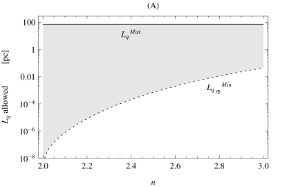
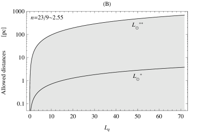
Figure 1: Panel A: $L_{q\oplus}^{Min}$ of eq.(15) and $L_{q}^{Max}$ of eq.(29). The gray zone represents the allowed characteristic-length scales of the model. We stress that $L_{q\odot}^{Min}$ is defined only if $n=(2m+1)/\ell$, as represented by the dotted line. Panel B: $L_{\odot}^{*}$ and $L_{\odot}^{**}$ of eq.(12). The gray zone represents here the allowed distances for the model.

At the same time two other typical lengths have been outlined in eq.(12) for the Solar System. $L_{\odot}^{*}$ represents the minimum distance to have post-Newtonian and Newtonian terms of the same order. While $L_{\odot}^{**}$ was defined according to the request that the weak-field expansion holds. Setting now $n=23/9\simeq 2.55$, one can show from eq.(15) and eq.(29) that the allowed scales are $0.0013\textrm{ pc}\;{\scriptstyle\lesssim}\;L_{q}\;{\scriptstyle\lesssim}\;71.72\textrm{ pc}$. In this range, $L_{\odot}^{*}$ and $L_{\odot}^{**}$ can be plotted as in Fig.1(B).

Summarizing, our analysis states a precise range of validity for the power-law $f(R)$ model we consider. Indeed, for a generic value of $n$ (i.e., not close to $2$ or $3$) the fundamental length of the model is constrained to range from the super Solar-System scale up to a sub-galactic one. Therefore, in agreement to eq.(9a), we have to search significant modification for the Newton law in gravitational system lying in this interval of length scales, like for instance, stellar clusters.

Acknowledgment: NC gratefully acknowledges the CPT - Université de la Mediterranée Aix-Marseille 2 and the financial support from “Sapienza” University of Rome.

References

• [1] T.P. Sotiriou and V. Faraoni, Rev. Mod. Phys. 82, 451 (2010).
• [2] A.F. Zakharov, A.A. Nucita, F. De Paolis and G. Ingrosso, Phys. Rev. D 74, 107101 (2006).
• [3] C.M. Will, Living Rev. Rel. 9, 3 (2006).
• [4] T. Chiba, T.L. Smith and A.L. Erickcek, Phys. Rev. D 75, 124014 (2007). V. Faraoni and N. Lanahan-Tremblay, Phys. Rev. D 77, 108501 (2008). H.J. Schmidt, Phys. Rev. D 78, 023512 (2008). S. Nojiri and S.D. Odintsov, Phys. Lett. B 657, 238 (2007). S.G. Turyshev, Annu. Rev. Nucl. Part. Sci. 58, 207 (2008). C.M. Will, Theory and Experiment in Gravitational Physics, Cambridge Univ. Press (1993).
• [5] O.M. Lecian and G. Montani, Class. Quant. Grav. 26, 045014 (2009).
• [6] M.T. Jaekel and S. Reynaud, in Gravitational waves and experimental gravity - Proc. of XLIIemes Rencontres de Moriond 2007, Eds. J. Dumarchez et al. (2007), pg. 271.
• [7] E.W. Kolb and M.S. Turner, The Early Universe, Westview Press (1990).
• [8] E. Komatsu et al., arXiv:1001.4538.
• [9] S. Nojiri and S.D. Odintsov, Phys. Rev. D 78, 046006 (2008).
• [10] E. Elizalde, S. Nojiri, S.D. Odintsov, D. Sรกez-Gรณmez and V. Faraoni, Phys. Rev. D 77, 106005 (2008).