Numerical simulations of the Fourier transformed Vlasov-Maxwell system in higher dimensions — Theory and applications

Abstract

We present a review of recent developments of simulations of the Vlasov-Maxwell system of equations using a Fourier transform method in velocity space. In this method, the distribution functions for electrons and ions are Fourier transformed in velocity space, and the resulting set of equations are solved numerically. In the original Vlasov equation, phase mixing may lead to an oscillatory behavior and sharp gradients of the distribution function in velocity space, which is problematic in simulations where it can lead to unphysical electric fields and instabilities and to the recurrence effect where parts of the initial condition recur in the simulation. The particle distribution function is in general smoother in the Fourier transformed velocity space, which is desirable for the numerical approximations. By designing outflow boundary conditions in the Fourier transformed velocity space, the highest oscillating terms are allowed to propagate out through the boundary and are removed from the calculations, thereby strongly reducing the numerical recurrence effect. The outflow boundary conditions in higher dimensions including electromagnetic effects are discussed. The Fourier transform method is also suitable to solve the Fourier transformed Wigner equation, which is the quantum mechanical analogue of the Vlasov equation for classical particles.

I Introduction

The Vlasov equation governs the dynamics of the distribution function of charged particles (electrons, ions) in the six-dimensional phase space, consisting of 3 velocity (or momentum) dimensions and 3 position dimensions, plus time. It offers an accurate description of a plasma in the collisionless limit, i.e., when the particles are affected by long-range electric and magnetic fields only, and when short-range fields from its nearest neighbors can be neglected.

The most common method to solve the Vlasov equation numerically is the Particle-In-Cell (PIC) method (Birdsall and Langdon, 1991; Matsumoto and Omura, 1993), where the Vlasov equation is solved by following the trajectories of a set of statistically distributed super-particles, which resolves the particle distribution functions in phase space. Each super-particle represents a large number of real particles. PIC simulations have proven to be extremely successful due to their relative simplicity and adaptivity. However, the statistical noise of PIC simulations sometimes overshadows the physical results, and for some problems, the low-density velocity tail of the particle distribution cannot be resolved with high enough accuracy by the super-particles.

Grid-based Vlasov solvers treat the particle distribution function as a phase fluid that is represented on a grid in both position and velocity (or momentum) space. The advantage with grid-based Vlasov solvers is that they do not give rise to statistical noise in the simulations, and that the dynamical range is larger than for PIC methods, so that the low-density velocity tail of the particle distribution can be resolved much more accurately. A disadvantage with grid-based Vlasov solvers in higher dimensions is that the full phase-space has to be represented on a numerical grid grid, which makes both the storage of the data in the computer’s memory, and the numerical calculations, extremely demanding. Another problem is the tendency of the distribution function to become oscillatory in velocity space due to phase mixing. This is the cause of Landau damping and other kinetic effects, but may lead to unphysical noise and recurrence effects in the numerical solution. This was recognized in early Vlasov simulations and special methods were devised to resolve this problem, including the Fourier-Fourier and Hermite expansion methods (Armstrong et al., 1970). Various other methods have also been developed for solving the Vlasov equation, the classical and widely used time-spitting method (Cheng and Knorr, 1976; Cheng, 1977) where a smoothing operator was applied to remove the highest oscillations in velocity space, a Van Leer dissipative scheme (Mangeney et al., 2002), the finite volume method (Elkina and Büchner, 2006), a back-substitution method for magnetized plasma (Schmitz and Grauer, 2006), etc. Several Eulerian grid-based solvers are reviewed and compared by Arber and Vann (2002) and Filbet and Sonnendrücker (2003).

One special category of methods are transform methods (Armstrong et al., 1970), where the particle distribution function is expressed as a sum or integral of basis functions in velocity space. The structuring of velocity space in this case leads to the excitation of higher and higher modes in the transformed velocity space, and special care must be taken when these excitations reach the highest mode represented in the numerical simulation. For example, for methods using Hermite polynomials to resolve the velocity space, the highest-order Hermite polynomials is designed to absorb the oscillations in velocity space (Knorr and Shoucri, 1974; Gibelli and Shizgal, 2006), thereby reducing numerical recurrence effects strongly. Klimas (1987) and Klimas (1994) devised filtering methods for the Fourier-Fourier method to remove the highest oscillations in velocity space. (In the Fourier-Fourier method, the Vlasov equation is Fourier transformed both in velocity space and position space, and the resulting equation is solved numerically.) For the Fourier method in one, two and three dimensions, Eliasson (2001, 2002, 2003, 2007) designed absorbing boundary conditions at the largest Fourier mode in velocity space so that the highest oscillations in velocity space were removed from the solution. In this method, the Vlasov equation is Fourier transformed only in velocity space and not in position space, so that the electromagnetic fields enter by multiplications instead of convolutions in the transformed Vlasov equation. The Fourier transformed Vlasov equation is also interesting to study in its own respect. Some mathematical aspects of the Fourier transformed Vlasov equation are given by Neunzert (1971, 1984), and in their analytic and and simulation studies, Sedlacec and Nocera (1992, 2002) presented interpretations of the Landau damping, the time echo phenomenon, etc., in terms of imperfectly trapped (leaking) waves in the Fourier transformed velocity space.

The main topic of this paper is a the properties of the Vlasov equation and the Fourier transformed Vlasov equation. The full Vlasov-Maxwell system, and the Vlasov-Maxwell system Fourier transformed in velocity space are presented in section II. In section III, we discuss the properties of the Vlasov equation that makes simulations a challenging task. We note that oscillations of the particle distribution function in velocity space corresponds to wave packets in the Fourier transformed velocity space. Special attention is put on the absorbing artificial boundary conditions in the Fourier transformed velocity space, where the highest Fourier modes are absorbed and removed from the calculations. These boundary conditions have the following attractive features: (i) They substantially reduce the unphysical reflections at the artificial boundaries, thereby reducing unphysical noise and recurrence effects in simulations. (ii) The boundary conditions are local in time and involve only boundary points (but they are non-local along the boundary). (iii) The boundary conditions together with the interior differential equation defines a well-posed problem. Some examples of simulations of one-dimensional kinetic structures, electron and ion holes, are also discussed in section III. In section IV, we will briefly mention the discrete approximations used in the numerical simulations of the Fourier transformed Vlasov equation. Especially the important topics of the representation of particle velocities by the numerical scheme and how to choose domain and grid sizes in the Fourier transformed velocity space are discussed. In sections V and VI, we present the generalizations of the Fourier technique to two and three dimensions, respectively. Here the treatment of the spatially varying magnetic field has to be treated carefully in the design of absorbing boundary conditions int the Fourier transformed velocity space. We mention here that the well-posedness of the boundary conditions for the one-, two- and three-dimensional Fourier transformed Vlasov equation have been proved by energy estimates (Eliasson, 2001, 2002, 2007), where an energy norm is non-increasing in time. Finally, in chapter VII, we discuss extensions of the Vlasov equation to incorporate quantum and relativistic effects. The quantum analogue to the Vlasov equation is the Wigner equation, and we will see that the absorbing boundary conditions used for the Vlasov equation can be applied unchanged to the Wigner equation. For the relativistic Vlasov equation, the relativistic gamma factor enters into the Vlasov equation and leads to a convolution in the Fourier transformed velocity space. This convolution operator is non-local in space and may lead to non-local absorbing boundary conditions in space and time.

II The Vlasov-Maxwell system of equations

The non-relativistic Vlasov equation

$$\frac{\partial f_{\mathrm{\alpha}}}{\partial t}+\textbf{v}\cdot\boldsymbol{\nabla}_{x}f_{\mathrm{\alpha}}+\frac{\textbf{F}_{\mathrm{\alpha}}}{m_{\mathrm{\alpha}}}\cdot\boldsymbol{\nabla}_{v}f_{\mathrm{\alpha}}=0$$ (1)

where the Lorentz force is

$$\textbf{F}_{\mathrm{\alpha}}=q_{\mathrm{\alpha}}[{\bf E}+\textbf{v}\times({\bf B}+{\bf B}_{\mathrm{ext}})]$$ (2)

describes the evolution of the distribution function $f_{\mathrm{\alpha}}$ of electrically charged particles of type $\mathrm{\alpha}$ (e.g., “electrons” or “singly ionized oxygen ions”), each particle having the electric charge $q_{\mathrm{\alpha}}$ and mass $m_{\mathrm{\alpha}}$. Here, the magnetic field is separated into two parts, where ${\bf B}_{\mathrm{ext}}$ is an external magnetic field (e.g., the Earth’s geomagnetic field), and ${\bf B}$ is the self-consistent part of the magnetic field, created by the plasma. One Vlasov equation is needed for each species of particles.

The particles interact via the electromagnetic field. The charge and current densities, $\rho$ and j, act as sources of self-consistent electromagnetic fields according to the Maxwell equations

$$\boldsymbol{\nabla}\cdot{\bf E} =\frac{\rho}{\varepsilon_{0}}$$ (3)

$$\boldsymbol{\nabla}\cdot{\bf B} =0$$ (4)

$$\boldsymbol{\nabla}\times{\bf E} =-\frac{\partial{\bf B}}{\partial t}$$ (5)

$$\boldsymbol{\nabla}\times{\bf B} =\mu_{0}\textbf{j}+\frac{1}{c^{2}}\frac{\partial{\bf E}}{\partial t}$$ (6)

The charge and current densities are related to the particle number densities $n_{\mathrm{\alpha}}$ and mean velocities $\textbf{v}_{\mathrm{\alpha}}$ as

$$\rho =\sum_{\mathrm{\alpha}}q_{\mathrm{\alpha}}n_{\mathrm{\alpha}}$$ (7)

and

j $$=\sum_{\mathrm{\alpha}}q_{\mathrm{\alpha}}n_{\mathrm{\alpha}}\textbf{v}_{\mathrm{\alpha}}$$ (8)

respectively, where the particle number densities and mean velocities are obtained as moments of the particle distribution functions, as

$$n_{\mathrm{\alpha}}(\textbf{x},t) =\int_{-\infty}^{\infty}f_{\mathrm{\alpha}}(\textbf{x},\textbf{v},t)\,\mathrm{d}^{3}v$$ (9)

and

$$\textbf{v}_{\mathrm{\alpha}}\left(\textbf{x},t\right) =\frac{1}{n_{\mathrm{\alpha}}\left(\textbf{x},t\right)}\int_{-\infty}^{\infty}\textbf{v}f_{\mathrm{\alpha}}\left(\textbf{x},\textbf{v},t\right)\,\mathrm{d}^{3}v$$ (10)

respectively.

The Vlasov equation (1) together with the Maxwell equations (3)–(6) and the constitutive equations (7)–(10) form a closed, coupled system of nonlinear partial differential equations and integral equations.

II.1 The Fourier transformed Vlasov equation

By using the Fourier transform pair

$$f_{\mathrm{\alpha}}(\textbf{x},\textbf{v},t) =\int_{-\infty}^{\infty}\widehat{f}_{\mathrm{\alpha}}(\textbf{x},\boldsymbol{\eta},t)e^{-\mathrm{i}\boldsymbol{\eta}\cdot\textbf{v}}\,\mathrm{d}^{3}\eta$$ (11)

$$\widehat{f}_{\mathrm{\alpha}}(\textbf{x},\boldsymbol{\eta},t) =\frac{1}{(2\pi)^{3}}\int_{-\infty}^{\infty}f_{\mathrm{\alpha}}(\textbf{x},\textbf{v},t)e^{\mathrm{i}\boldsymbol{\eta}\cdot\textbf{v}}\,\mathrm{d}^{3}\eta$$ (12)

the velocity variable v is transformed into a new variable $\boldsymbol{\eta}$ and the distribution function $f(\textbf{x},\textbf{v},t)$ is changed to a new, complex valued, function $\widehat{f}(\textbf{x},\boldsymbol{\eta},t)$, which obeys the transformed Vlasov equation

$$\frac{\partial\widehat{f}_{\mathrm{\alpha}}}{\partial t}-\mathrm{i}\boldsymbol{\nabla}_{x}\cdot\boldsymbol{\nabla}_{\eta}\widehat{f}_{\mathrm{\alpha}}-\frac{q_{\mathrm{\alpha}}}{m_{\mathrm{\alpha}}}\big{(}\mathrm{i}{\bf E}\cdot\boldsymbol{\eta}\widehat{f}_{\mathrm{\alpha}}+\boldsymbol{\nabla}_{\eta}\cdot\{[({\bf B}+{\bf B}_{\mathrm{ext}})\times\boldsymbol{\eta}]\widehat{f}_{\mathrm{\alpha}}\}\big{)}=0$$ (13)

The nabla operators $\boldsymbol{\nabla}_{x}$ and $\boldsymbol{\nabla}_{\eta}$ denote differentiation with respect to x and $\boldsymbol{\eta}$, respectively.

Equation (13) together with the Maxwell equations (3)–(6) and the constitutive equations (7)–(8) where the particle number densities and mean velocities are obtained as

$$n_{\mathrm{\alpha}}(\textbf{x},t) =(2\pi)^{3}\widehat{f}_{\mathrm{\alpha}}(\textbf{x},\textbf{0},t)$$ (14)

and

$$\textbf{v}_{\mathrm{\alpha}}(\textbf{x},t) =-\mathrm{i}\frac{(2\pi)^{3}}{n_{\mathrm{\alpha}}(\textbf{x},t)}\left[\boldsymbol{\nabla}_{\eta}\widehat{f}_{\mathrm{\alpha}}(\textbf{x},\boldsymbol{\eta},t)\right]_{\boldsymbol{\eta}=\textbf{0}}$$ (15)

respectively, form a new closed set of equations. One can note that the integrals over infinite v space in Eqs. (9) and (10) have been converted to evaluations in $\boldsymbol{\eta}$ space in Eqs. (14 and 15). The factor $(2\pi)^{3}$ in Eqs. (12), (14) and (15) is valid for three velocity dimensions. For $n$ velocity dimensions this factor is $(2\pi)^{n}$.

II.2 Invariants of the Vlasov-Maxwell system

The Vlasov equation (1) coupled with (3)–(6) conserves the energy norm

$$\|f_{\alpha}\|^{2} =\int\int f_{\alpha}^{2}\,\mathrm{d}^{3}v\,\mathrm{d}^{3}x,$$ (16)

the total number of particles

$$N_{\alpha} =\int\int f_{\alpha}\,\mathrm{d}^{3}v\mathrm{d}^{3}x,$$ (17)

the total linear momentum

$$\mathbf{p} =\int\left[\int{\bf v}(m_{i}f_{i}+m_{e}f_{e})\,\mathrm{d}^{3}v+\varepsilon_{0}{{\bf E}}\times{{\bf B}}\right]\,\mathrm{d}^{3}x,$$ (18)

and the total energy

$$W =\int\left[\int\frac{1}{2}{\textbf{v}}^{2}(m_{i}f_{i}+m_{e}f_{e})\,\mathrm{d}^{3}v+\frac{1}{2}\left(\varepsilon_{0}{{\bf E}}^{2}+\frac{{{\bf B}}^{2}}{\mu_{0}}\right)\right]\,\mathrm{d}^{3}x.$$ (19)

The corresponding invariants for the Fourier-transformed Vlasov-Maxwell system (13) and (3)–(6) are:

$$\|\widehat{f}_{\alpha}\|^{2} =\frac{1}{(2\pi)^{3}}\int\int|\widehat{f}_{\alpha}|^{2}\,\mathrm{d}^{3}\eta\,\mathrm{d}^{3}x,$$ (20)

$$N_{\alpha} =\int(2\pi)^{3}(\widehat{f}_{\alpha})_{{\boldsymbol{\eta}}=0}\,\mathrm{d}^{3}x,$$ (21)

$$\mathbf{p} =\int[-\mathrm{i}(2\pi)^{3}\boldsymbol{\nabla}_{\boldsymbol{\eta}}(m_{\rm i}f_{\rm i}+m_{\rm e}f_{\rm e})_{\boldsymbol{\eta}=0}+\varepsilon_{0}{{\bf E}}\times{{\bf B}}]\,\mathrm{d}^{3}x,$$ (22)

and

$$W =\int\bigg{[}-\frac{1}{2}(2\pi)^{3}\nabla_{\boldsymbol{\eta}}^{2}(m_{\rm i}f_{\rm i}+m_{\rm e}f_{\rm e})_{\boldsymbol{\eta}=0}+\frac{1}{2}\left(\varepsilon_{0}{{\bf E}}^{2}+\frac{{{\bf B}}^{2}}{\mu_{0}}\right)\bigg{]}\,\mathrm{d}^{3}x,$$ (23)

respectively, where the norm (20) follows from (16) via the Parseval relation. These invariants can be used to check the accuracy of the numerical scheme. When the system is restricted to a bounded domain in $\boldsymbol{\eta}$ space with appropriate boundary conditions (discussed in Section VI.2 below), the norm $\|\widehat{f}_{\alpha}\|^{2}$ will be a non-increasing, positive function of time, while the other three quantities will still be conserved.

II.3 The electrodynamic scalar and vector potentials

The Maxwell equations (3)–(6) can be written in terms of the scalar and vector potentials $\Phi$ and ${\bf A}$, which are related to the electromagnetic field as

$${\bf E} =-\boldsymbol{\nabla}\Phi-\frac{\partial{\bf A}}{\partial t}$$ (24)

$${\bf B} ={\bf B}_{0}+\boldsymbol{\nabla}\times{\bf A},$$ (25)

where ${\bf B}_{0}$ is the external magnetic field. Introducing these expressions into Eqs. (3)–(6), and choosing the Lorentz condition,

$$\boldsymbol{\nabla}\cdot{\bf A}+\frac{1}{c^{2}}\frac{\partial\Phi}{\partial t}=0$$ (26)

yields the electrodynamic waves equations

$$\frac{1}{c^{2}}\frac{\partial^{2}\Phi}{\partial t^{2}}-\nabla^{2}\Phi =\frac{\rho}{\varepsilon_{0}}$$ (27)

$$\frac{1}{c^{2}}\frac{\partial^{2}{\bf A}}{\partial t^{2}}-\nabla^{2}{\bf A} =\mu_{0}\textbf{j}.$$ (28)

In this description, the divergence of the magnetic field is zero, since the divergence of the right hand side of Eq. (25) is zero by the vector relation $\boldsymbol{\nabla}\cdot(\boldsymbol{\nabla}\times{\bf A})=0$. The divergence of the electric field can be set to the correct value by using the Maxwell equation for the divergence of the electric field (3) together with Eq. (24), yielding

$$\boldsymbol{\nabla}\cdot{\bf E} =-\nabla^{2}\Phi-\boldsymbol{\nabla}\cdot\frac{\partial{\bf A}}{\partial t}=\frac{\rho}{\varepsilon_{0}}$$ (29)

or

$$-\nabla^{2}\Phi =\frac{\rho}{\varepsilon_{0}}+\boldsymbol{\nabla}\cdot\frac{\partial{\bf A}}{\partial t}$$ (30)

This equation for $\Phi$ conserves the divergence of the electric field.

By introducing a separate variable $\boldsymbol{\Gamma}$ for the time derivative of the vector potential ${\bf A}$, the wave equations (28) and (30) can be rewritten in a first-order system with respect to time,

$$\frac{\partial{\bf A}}{\partial t} =\boldsymbol{\Gamma} \frac{\partial\boldsymbol{\Gamma}}{\partial t} =c^{2}(\nabla^{2}{\bf A}+\mu_{0}\textbf{j})$$ (31)

$$-\nabla^{2}\Phi =\frac{\rho}{\varepsilon_{0}}+\boldsymbol{\nabla}\cdot\boldsymbol{\Gamma}$$ (32)

and the electric and magnetic fields are calculated as

$${\bf E} =-\boldsymbol{\nabla}\Phi-\boldsymbol{\Gamma}$$ (33)

and

$${\bf B} =\boldsymbol{\nabla}\times{\bf A}$$ (34)

respectively, in the new variables.

The system (31)–(34) produces physical electric and magnetic fields regardless of the initial conditions on ${\bf A}$ and $\boldsymbol{\Gamma}$, in the sense that the first two Maxwell equations for the divergences (3)–(4) are fulfilled. Therefore, a consistent numerical scheme will also produce physical solutions, up to the local truncation error of the numerical scheme, even after a long time; no artificial electric and magnetic charges are created and accumulated by the numerical scheme, which could be the case if the two last Maxwell equations (5)–(6) are integrated numerically in time. This general property of the system is an advantage, since it is not necessary to use special, divergence-conserving schemes Wagner and Schneider (1998) to solve these equations, and it therefore opens up the possibility to switch between different numerical methods without having to pay too much attention to the divergences of the electromagnetic field. In complicated geometries, it may be a disadvantage that an elliptic equation (32) has to be solved numerically to obtain the potential $\Phi$, while in the simple geometries considered here, with periodic boundary conditions, Eq. (32) is efficiently solved by means of Fourier transform techniques.

II.4 The reduction of spatial and velocity dimensions

In the study of problems with certain symmetries, it is sometimes possible to make a choice of the coordinate system so that the the problem can be analyzed in a smaller number of dimensions. Numerically, this is very convenient because unnecessary information is removed from the problem and a smaller number of sampling points is needed to represent the solution on a numerical grid.

One such assumption is that the problem is homogeneous in one or more dimensions, in which case the derivatives in these dimensions vanish. In the study of plane waves in plasma, the number of dimensions in $\textbf{x}=(x_{1},x_{2},x_{3})$ space can be reduced to one dimension, $\textbf{x}=(x_{1},0,0)$, so that only derivatives with respect to $x_{1}$ (and not $x_{2}$ and $x_{3}$) remain. In this manner, the Vlasov equation can be reduced from three spatial and velocity dimensions, to one spatial and three velocity dimensions, plus time.

For the non-relativistic Vlasov equation, it turns out that it is also possible to reduce the number of velocity dimensions, but in a different manner than for the spatial dimensions. For electrostatic electron waves in an unmagnetized plasma, the reduction to one spatial dimension $x_{1}$ also leads to that terms containing factors of $v_{2}$ and $v_{3}$, and derivatives with respect to $v_{2}$ and $v_{3}$, also vanish, giving rise to the system

$$\frac{\partial f}{\partial t}+v_{1}\frac{\partial f}{\partial x_{1}}-\frac{eE_{1}}{m_{\mathrm{e}}}\frac{\partial f}{\partial v_{1}}=0$$ (35)

$$\frac{\partial E_{1}}{\partial x_{1}}=\frac{e}{\varepsilon_{0}}\bigg{[}n_{0}-\int_{-\infty}^{\infty}\int_{-\infty}^{\infty}\int_{-\infty}^{\infty}f(x_{1},v_{1},v_{2},v_{3},t)\,\mathrm{d}v_{1}\,\mathrm{d}v_{2}\,\mathrm{d}v_{3}\bigg{]}$$ (36)

The dependence on $(v_{2},v_{3})$ only appears in the integral over all velocity space for calculating the electric field $E_{1}$. Similarly, for waves in a magnetized plasma, propagating in the $(x_{1},x_{2})$ plane perpendicular to the magnetic field directed in the $x_{3}$ direction and with the electric field directed in the $(x_{1},x_{2})$ plane perpendicular to the magnetic field, any dependencies on the distribution in $v_{3}$ vanish in the Vlasov equation, and one has one Vlasov equation in $(x_{1},x_{2},v_{1},v_{2},t)$ space for each value on $v_{3}$. In these cases, it is possible (and convenient) to reduce the number of dimensions also in v space.

In the study of collective phenomena in plasma, the electromagnetic fields do not depend explicitly on the exact velocity distribution of particles but on the charge and current densities in x space, calculated as integrals (moments) of the distribution function. This makes it possible to reduce the number of velocity dimensions in the Vlasov equation. For the case of electrostatic waves in an unmagnetized plasma discussed above, it is simple to show that linear combinations of distribution functions with different $(v_{2},v_{3})$ are solutions to the one-dimensional Vlasov equation (35), because these distribution functions separately are solutions to the same Vlasov equation. In particular, taking the limit of a continuous “linear combination,” the one-dimensional distribution function

$$f^{1\mathrm{D}}(x_{1},v_{1},t)=\int_{-\infty}^{\infty}\int_{-\infty}^{\infty}f(x_{1},v_{1},v_{2},v_{3},t)\,\mathrm{d}v_{2}\,\mathrm{d}v_{3}$$ (37)

is a solution to the one-dimensional Vlasov equation (35) because the function $f(x_{1},v_{1},v_{2},v_{3},t)$ is a solution to the the Vlasov equation (35) for each value on $(v_{2},v_{3})$. The electric field is calculated from Eq. (36) where, by Eq (37),

$$\int_{-\infty}^{\infty}\int_{-\infty}^{\infty}\int_{-\infty}^{\infty}f\,\mathrm{d}v_{1}\,\mathrm{d}v_{2}\,\mathrm{d}v_{3}=\int_{-\infty}^{\infty}f^{1\mathrm{D}}\,\mathrm{d}v_{1}$$ (38)

and the resulting one-dimensional Vlasov equation coupled with Gauss’ law is

$$\frac{\partial f^{1\mathrm{D}}}{\partial t}+v_{1}\frac{\partial f^{1\mathrm{D}}}{\partial x_{1}}-\frac{eE_{1}}{m_{\mathrm{e}}}\frac{\partial f^{1\mathrm{D}}}{\partial v_{1}}=0$$ (39)

$$\frac{\partial E_{1}}{\partial x_{1}}=\frac{e}{\varepsilon_{0}}\bigg{[}n_{0}-\int_{-\infty}^{\infty}f^{1\mathrm{D}}(x_{1},v_{1},t)\,\mathrm{d}v_{1}\bigg{]}$$ (40)

for the unknown function $f^{1\mathrm{D}}$.

For waves propagating perpendicularly to a magnetic field, mentioned above, it is possible to derive the two-dimensional Vlasov-Maxwell system, which depends on the distribution functions in the form

$$f^{2\mathrm{D}}(x_{1},x_{2},v_{1},v_{2},t)=\int_{-\infty}^{\infty}f(x_{1},x_{2},v_{1},v_{2},v_{3},t)\,\mathrm{d}v_{3}$$ (41)

For waves propagating with some angle to the magnetic field, it is more difficult to reduce the number of velocity dimensions in the manner described above, since all three velocity components will appear explicitly in the resulting Vlasov equation. Even so, the reduction of the number of velocity dimensions for the Vlasov equation has been done also for this case, in which a full Vlasov kinetic description is maintained only along one “dominant” spatial coordinate, and with the perpendicular dimensions modeled by reduced moment-based methods (Newmann et al., 2004).

III Properties of the Vlasov equation

A well-known property of the Vlasov equation is that an initially smooth distribution function which evolves in time may become increasingly oscillatory in velocity space due to phase mixing of the distribution function. This leads to Landau damping and other kinetic effects, but it also makes the numerical solution of the Vlasov equation a challenging task (Armstrong et al., 1970; Cheng and Knorr, 1976). We here discuss the main features of the Vlasov equation and the numerical difficulties arising from the phase mixing effects. The phase mixing and oscillatory behavior of the Vlasov equation in velocity space leads to wave packets in the Fourier transformed velocity space, which points to the idea to absorb the highest Fourier modes via boundary conditions in the Fourier transformed Vlasov equation.

III.1 The filamentation in velocity space and the numerical recurrence effect

The behavior of the Vlasov equation is illustrated by the one-dimensional Vlasov equation for electrons with stationary, singly charged ions, coupled with Gauss’ law for the electrostatic field,

$$\frac{\partial f_{e}}{\partial t}+v\frac{\partial f_{e}}{\partial x}-\frac{eE}{m_{e}}\frac{\partial f_{e}}{\partial v}=0,$$ (42)

$$\frac{\partial E}{\partial x}=\frac{e}{\varepsilon_{0}}\bigg{[}n_{0}-\int_{-\infty}^{\infty}f_{e}(x,v,t)\,\mathrm{d}v\bigg{]},$$ (43)

describing the evolution of the electron distribution function $f_{e}$ in a self-consistent electric field $E$, where $n_{0}$ is the equilibrium electron (and ion) number density, $e$ is the magnitude of the electron charge, $m_{e}$ is the electron mass, and $\varepsilon_{0}$ is the electric vacuum permittivity. It can be cast into the dimensionless form

$$\frac{\partial f_{e}}{\partial t}+v\frac{\partial f_{e}}{\partial x}-E\frac{\partial f_{e}}{\partial v}=0,$$ (44)

$$\frac{\partial E}{\partial x}=1-\int_{-\infty}^{\infty}f_{e}(x,v,t)\,\mathrm{d}v,$$ (45)

were the distribution function $f_{e}$ is normalized by $n_{0}/v_{th,e}$, time $t$ by $\omega_{pe}^{-1}$, space $x$ by $r_{De}$, velocity $v$ by $v_{th,e}$, and the electric field $E$ by $v_{th,e}^{2}m_{e}/er_{De}$. Here $\omega_{pe}=(n_{0}e^{2}/\varepsilon_{0}m_{e})^{1/2}$ is the electron plasma frequency, $r_{De}=(k_{B}T_{e}\varepsilon_{0}/n_{0}e^{2})^{1/2}$ is the electron Debye length, $v_{th,e}=(k_{B}T_{e}/m_{e})^{1/2}$ is the electron thermal speed, $T_{e}$ is the electron temperature, and $k_{B}$ is Boltzmann’s constant.

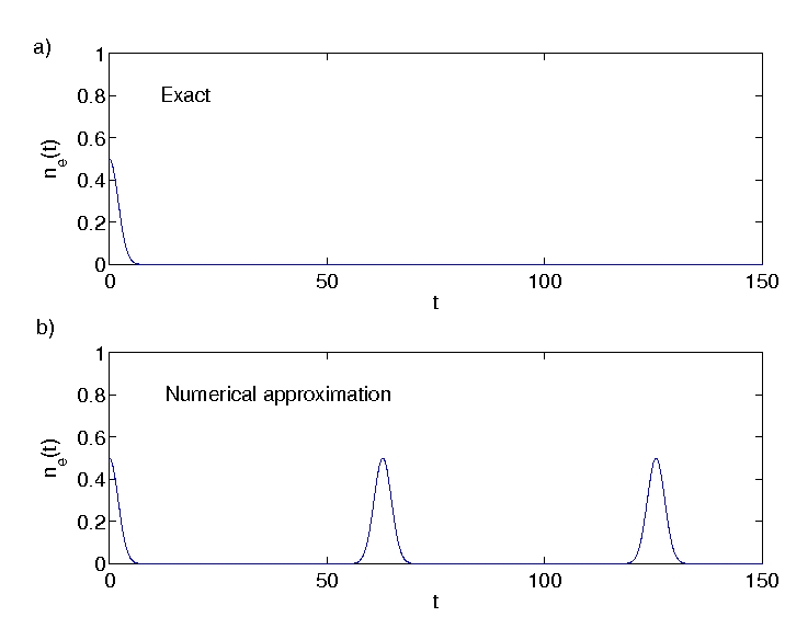
Figure 1: a) Exact and b) numerical approximation of the electron number density $n_{e}$. One can see a numerical recurrence effect with periodicity ${T_{\rm recurrence}=2\pi/(k_{x}\,\Delta v)\approx 62.8}$.

To illustrate the main numerical difficulty of the Vlasov equation, we consider the reduced, free-streaming problem

$$\frac{\partial f}{\partial t}+v\frac{\partial f}{\partial x}=0,\qquad f(x,v,t=0)=\frac{A}{\sqrt{2\pi}}\cos(k_{x}x)\exp(-\frac{v^{2}}{2})$$ (46)

which has the exact solution

$$f=(2\pi)^{-1/2}A\cos[{k_{x}}(x-{vt})]\exp(-v^{2}/2).$$ (47)

This solution becomes more and more oscillatory in the velocity space with increasing time due to the $kvt$ term inside the cosinus function. We note that the distribution function $f$ does not decay in time, but, due to phase mixing between positive and negative values of $f$, the number density

$$n_{e}=\int f\,dv=A{\exp(-k_{x}^{2}t^{2}/2)}\cos(k_{x}x),$$ (48)

decays super-exponentially fast with time. Assume now that we have the exact solution $f$ of the electron distribution function, and want to calculate the electron number density numerically via a sum representation of the integral over velocity space. If we resolve velocity space with an equidistant grid as $v=v_{j}=j\Delta v$, $j=0$, $\pm 1$, $\pm 2$, …, $\pm M$, where $M$ is a large integer, then a numerical approximation of the electron number density is

$$n_{e}\approx\sum_{j=-M}^{M}(2\pi)^{-1/2}A\cos[{k_{x}}(x-{j\Delta vt})]\exp(-j^{2}\Delta v^{2}/2)\,\Delta v,$$ (49)

which turns out to be periodic in time with periodicity ${T_{\rm recurrence}=2\pi/(k_{x}\,\Delta v)}$. For example, for $k_{x}=0.5$ and $\Delta v=0.2$, we have ${T_{\rm recurrence}=2\pi/(k_{x}\,\Delta v)\approx 62.8}$. While the exact number density decays super-exponentially, we see in Fig 1 that in the numerical approximation, the initial condition recurs periodically with periodicity ${T_{\rm recurrence}\approx 62.8}$. This is the recurrence effect. It is in fact impossible to represent the solution on the grid after a finite time due to the Nyquist-Shannon sampling theorem, which states that one needs more than two grid points per wavelength to represent the solution an equidistant grid. Here we see from Eq. (47) that the “wavelength” in velocity space is $\lambda_{v}=2\pi/(k_{x}t)$. Hence, the sampling theorem $\lambda_{v}/\Delta v>2$ for representing the distribution function on the grid is violated for times $t\geq\pi/(k_{x}\Delta v)=T_{\rm recurrence}/2$.

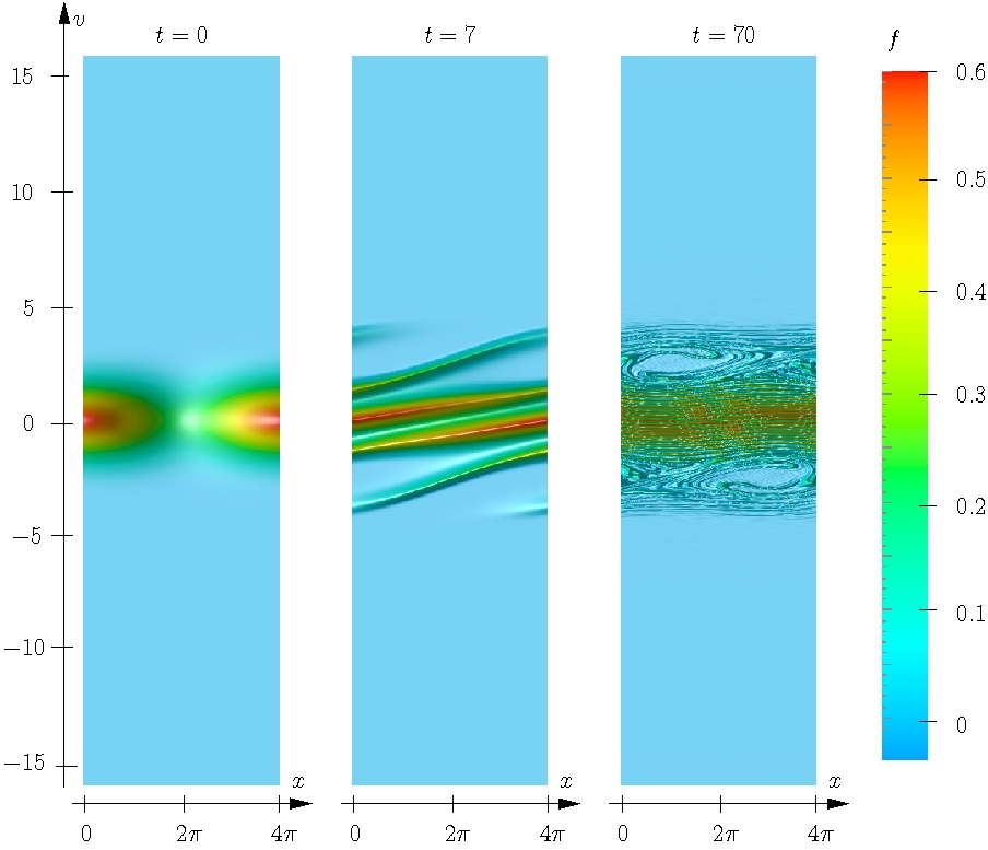
(a) The distribution function $f(x,v,t)$

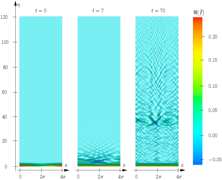
(b) The real part of the Fourier transformed distribution function $\widehat{f}(x,\eta,t)$

Figure 2: Phase space plots of the electron distribution function $f(x,v,t)$ and the real part of the Fourier transformed distribution function $\widehat{f}(x,\eta,t)$ at different times. After Eliasson (2006).

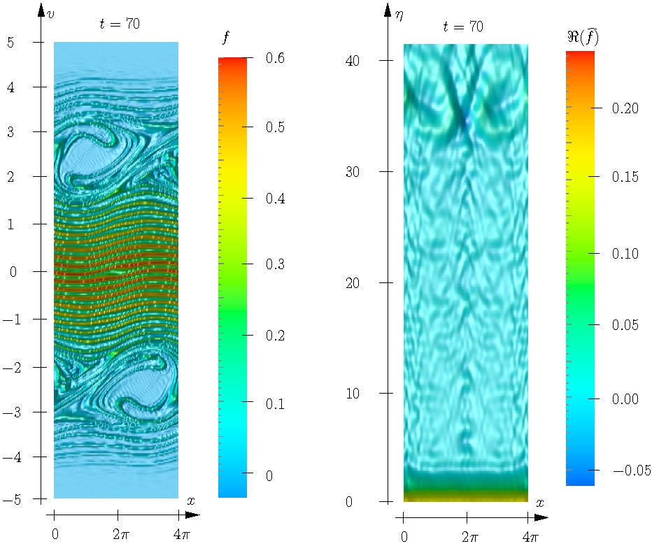
Figure 3: A closeup of the distribution function $f(x,v,t)$ and of the real part of the Fourier transformed distribution function $\widehat{f}(x,\eta,t)$ at the time $t=70$. After Eliasson (2006).

We now return to the system (44)–(45). By employing the Fourier transform pair

$$f(x,v,t) =\int_{-\infty}^{\infty}\widehat{f}(x,\eta,t)\mathrm{e}^{-\mathrm{i}\eta v}\,\mathrm{d}\eta$$ (50)

$$\widehat{f}(x,\eta,t) =\frac{1}{2\pi}\int_{-\infty}^{\infty}f(x,v,t)e^{\mathrm{i}\eta v}\,\mathrm{d}v$$ (51)

the system (44)–(45) is transformed into a new set of equations

$$\frac{\partial\widehat{f}}{\partial t}-\mathrm{i}\frac{\partial^{2}\widehat{f}}{\partial x\partial\eta}+\mathrm{i}E\eta\widehat{f}=0$$ (52)

$$\frac{\partial E(x,t)}{\partial x}=1-2\pi\widehat{f}(x,\eta,t)_{\eta=0}$$ (53)

for the Fourier transformed distribution function $\widehat{f}(x,\eta,t)$. Here $\widehat{f}$ is normalized by $n_{0}$ and the Fourier transformed velocity variable $\eta$ is normalized by $v_{{\rm th,e}}^{-1}$, while the other variables are normalized in the same manner as in Eqs. (44)–(45). As initial conditions for Eq. (44), we will use (Armstrong et al., 1970; Cheng and Knorr, 1976)

$$f(x,v,0)=[1+A\cos(k_{x}x)]f_{0}(v),$$ (54)

with $A=0.5$, $k_{x}=0.5$, and $f_{0}(v)=(2\pi)^{-1/2}\exp\left(-v^{2}/2\right)$; see Fig. 2(a) at $t=0$. The corresponding initial condition for the Fourier transformed Vlasov equation (52), shown at $t=0$ in Fig. 2(b), is

$$\widehat{f}(x,\eta,0)=[1+A\cos(k_{x}x)]\widehat{f}_{0}(\eta),$$ (55)

with $\widehat{f}_{0}(\eta)=(2\pi)^{-1}\exp(-\eta^{2}/2)$. We used the method of Eliasson (2001) to solve the system (44)–(45). The simulation domain was set to ${0\leq x\leq 4\pi}$ and $0\leq\eta\leq 120$ with $N_{x}=200$, $N_{\eta}=600$, and the time domain was $0\leq t\leq 70$ with $N_{t}=35000$ and $\Delta t=0.002$. The numerical dissipation parameter in $x$ space was set to ${\delta=0.001}$.

As can be seen in Fig. 2(a), the solution has at $t=7$ formed filaments with large gradients in velocity space. At $t=70$, the gradients have further steepened, and two Bernstein-Green-Kruskal (BGK) waves have been formed. A closeup of the solution is shown in the left-hand panel of Fig. 3. The initially smooth solution has evolved into an oscillatory solution with steep gradients, primarily in $v$ space but also in $x$ space. As a contrast, the Fourier transformed solution $\widehat{f}(x,\eta,t)$, displayed in Fig. 2(b) for the same times as in Fig. 2(a), does not become oscillatory in velocity space. Instead, wave packets are formed and are propagating away from the origin $\eta=0$ in the Fourier transformed velocity space.

The smooth solution in the Fourier transformed velocity space is a desirable property for numerical approximations of the Vlasov equation. It is possible to give an upper bound on the derivatives in $\eta$ space and on numerical truncation errors for numerical schemes that approximate the $\eta$ derivatives, which is not possible in the original velocity $v$ space. By inspection of the three panels in Fig. 2(a), one can see that the solution has significantly non-zero values only in the velocity interval $v=-5$ to $v=5$. This suggests that the Vlasov equation in the Fourier transformed space has a smooth solution. If one assumes that the solution in Fig. 2(a) for all times vanishes as a Gaussian function for large $v$, with the estimate

$$\left|{f(x,v,t)}\right|<C\exp(-\gamma v^{2})$$ (56)

for some positive constants $C$ and $\gamma$, then the $\eta$ derivatives of the Fourier transformed solution are bounded as

$$\begin{split}&\bigg{|}\frac{\partial^{n}}{\partial\eta^{n}}\widehat{f}(x,\eta,t)\bigg{|}=\mbox{[Use Eq.~{}(\ref{Fourier2})]}=\bigg{|}\frac{1}{2\pi}\int_{-\infty}^{\infty}(\mathrm{i}v)^{n}e^{\mathrm{i}\eta v}f(x,v,t)\,\mathrm{d}v\bigg{|}\\ &<\mbox{[Use the triangle inequality]}<\frac{1}{2\pi}\int_{-\infty}^{\infty}|(\mathrm{i}v)^{n}e^{\mathrm{i}\eta v}f(x,v,t)|\,\mathrm{d}v\\ &=\frac{1}{2\pi}\int_{-\infty}^{\infty}|v|^{n}|f(x,v,t)|\,\mathrm{d}v<\mbox{[By Eq.~{}(\ref{f_estimate})]}\\ &<\frac{1}{2\pi}\int_{-\infty}^{\infty}|v|^{n}C\exp(-\gamma v^{2})\,\mathrm{d}v=\frac{1}{2\pi}\frac{C}{\gamma^{(n+1)/2}}a_{n}\end{split}$$ (57)

where the constant

$$a_{n}=\left\{\begin{array}[]{ll}\sqrt{\pi}\,2^{-n/2}(n-1)!!,&{\mbox{$n$ even}}\\ $[(n-1)/2]!$,&{\mbox{$n$ odd}}\end{array}\right.$$ (58)

and where the symbols $!$ for the factorial and $!!$ for the semi-factorial have their usual meaning. Thus, by the assumption (56) for $f(x,v,t)$ it follows that $\widehat{f}(x,\eta,t)$ is infinitely differentiable with respect to $\eta$ with the estimate (57) for the derivatives. It is therefore possible to make an error estimate of the truncation error of a difference scheme used to approximate the $\eta$ derivative in Eq. (52). The 4th-order compact Padé difference scheme, which is used here to perform numerical approximations of the first derivatives in $\boldsymbol{\eta}$ space (See Section IV below) has a truncation error of size

$$|\varepsilon|\leq\frac{1}{120}\Delta\eta^{4}\max\bigg{|}\frac{\partial^{5}\widehat{f}}{\partial\eta^{5}}\bigg{|}$$ (59)

where the fifth derivative gives $n=5$ in formula (57). This gives the estimate

$$|\varepsilon|<\frac{1}{2\pi}\frac{\Delta\eta^{4}}{60}\frac{C}{\gamma^{3}}$$ (60)

for the truncation error. It is thus possible to make an error estimate for the numerical differentiation in the Fourier transformed velocity $\eta$ space in Eq. (52), which is not possible for a numerical differentiation in the original velocity $v$ space in Eq. (44). In the closeup of the solution at time $t=70$, displayed in right panel of Fig. 3, a wave packet can clearly be seen at $\eta\approx 35$, which corresponds to the “frequency” of the oscillations in velocity space, seen in the left panel of Fig. 3. Since the wave packet is decoupled from the origin $\eta=0$ where the electric field is calculated, it can be removed from the calculation without immediately affecting the value of the electric field. The wave packets eventually reach the artificial boundary at $\eta=\eta_{\mathrm{max}}=120$; see the right panel of Fig. 2(b), where they are absorbed, as described in the next section.

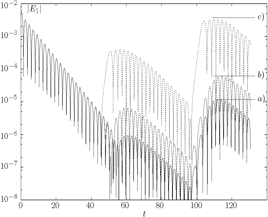
Figure 4: The electric field for small-amplitude electrostatic waves. a) and b): outflow boundary conditions in $\eta$ space. c): $\widetilde{f}$ set to zero at boundary $\eta=\eta_{max}$. After Eliasson (2001).

III.2 Outflow boundary conditions in Fourier transformed velocity space

The idea developed in (Eliasson, 2001, 2002, 2007) is to solve the Vlasov equation in the Fourier transformed velocity space and to design absorbing boundary conditions at the largest component; wave packets that reach the artificial boundary in the Fourier transformed velocity space are allowed to travel over the boundary and to be removed from the solution, while incoming waves are set to zero at the boundary. In this manner a weakly dissipative term is introduced in the Vlasov equations, which removes only the highest oscillations in velocity space. By setting the artificial boundary further away from the origin in the Fourier transformed velocity space, finer structures is resolved in velocity space.

The idea can be illustrated with the reduced problem

$$\frac{\partial\widehat{f}}{\partial t}-i\frac{\partial^{2}\widehat{f}}{\partial x\partial\eta}=0.$$ (61)

A Fourier transform in space ($\partial/\partial x\rightarrow ik$) gives the hyperbolic equation

$$\frac{\partial\widetilde{f}}{\partial t}+k_{x}\frac{\partial\widetilde{f}}{\partial\eta}=0,$$ (62)

which has solutions of the form $\widetilde{f}=\widetilde{f}_{0}(\eta-k_{x}t)$. Well-posed outflow boundary conditions for Eq. (62) in $\eta$ space are found by setting $\widehat{f}$ to zero at $\eta=\eta_{max}$ if $k_{x}<0$ and to zero at $\eta=-\eta_{max}$ if $k_{x}>0$. It can be expressed as $\widetilde{f}=H(k_{x})\widetilde{f}$ at $\eta=\eta_{max}$ and $\widetilde{f}=H(-k_{x})\widetilde{f}$ at $\eta=-\eta_{max}$ where $H$ is the Heaviside function, here defined as $H(k_{x})=0$ for $k_{x}\leq 0$ and $H(k_{x})=1$ for $k_{x}>0$. Inverse Fourier transforming the boundary conditions, we obtain well-posed outflow boundary conditions for $\widehat{f}$,

$$\widehat{f}={\rm F}^{-1}[H(k_{x}){\rm F}\widehat{f}]\quad\mbox{at }\eta=\eta_{max}$$ (63)

and

$$\widehat{f}={\rm F}^{-1}[H(-k_{x}){\rm F}\widehat{f}]\quad\mbox{at }\eta=-\eta_{max}$$ (64)

where ${\rm F}$ and ${\rm F}^{-1}$ are the forward and inverse spatial Fourier transforms.

It turns out that the outflow boundary condition (63) also works well for the complete Fourier transformed system (52)–(53). Figure 4 shows a simulation with a small-amplitude wave in the initial condition so that we have an almost linear problem. The wavenumber is set to $k_{x}=0.5$ so that the wave is strongly Landau damped. We are comparing cases where we have used the outflow boundary condition (63) at $\eta=\eta_{max}=30$ [panels a) and b) in Fig. 4] with a case where we simply set $\widetilde{f}$ to zero at the boundary [panel c)]. [A denser grid in $\eta$ space is used in a) compared to b).] In the simulation in Fig. 4, the amplitude of the wave is initially decreasing exponentially as expected from linear Vlasov theory. At $t\approx 60\omega_{pe}^{-1}$, there is a weak recurrence of the waves, and at $t\approx 120\omega_{pe}^{-1}$ a stronger recurrence takes place. We see that the recurrence phenomenon is much weaker for case a) and b) where outflow boundary conditions were used in $\eta$ space, while in case c), where the distribution function was set to zero at the $\eta$ boundary, the amplitude of the recurring wave at $t=120\,\omega_{pe}^{-1}$ is of the same order as in the initial condition. For the case c) the numerical results would be useless for a nonlinear problem after the recurrence has taken place at $t=120\,\omega_{pe}^{-1}$, while for the other cases the linear Landau damping effects are reasonably well represented and a nonlinear problem could be run beyond the recurrence time.

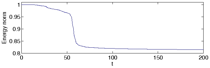
Figure 5: Large amplitude case. Time development of the energy integral $||\widetilde{f}||_{2}$ in Eq. (66), normalized by its initial value.

An interesting question is what is flowing out at the outflow boundary in $\eta$ space. It is easy to show that the energy (entropy) integrals $||f||^{2}$ and $||\widehat{f}||^{2}$ are conserved in time, where

$$||f||^{2}=\int_{0}^{L}\!\!\int f^{2}dv\,dx\mbox{ and }||\widehat{f}||^{2}=\int_{0}^{L}\!\!\int|\widehat{f}|^{2}d\eta\,dx.$$ (65)

if periodic boundary conditions are used in space. They are related as $||f||^{2}=2\pi||\widehat{f}||^{2}$ via Parseval’s relation. With the outflow boundary condition (63) in $\eta$ space, it was shown by Eliasson (2001) for the one-dimensional case that the energy integral

$$||\widehat{f}||^{2}=\int_{0}^{L}\!\!\int_{-\eta_{max}}^{\eta_{max}}|\widehat{f}|^{2}d\eta\,dx$$ (66)

is non-increasing in time, i.e. $d||\widehat{f}||^{2}/dt\leq 0$. In fact, due to that $f$ is real valued, the symmetry condition $\widehat{f}(x,-\eta,t)=\widehat{f}^{*}(x,\eta,t)$ was used by Eliasson (2001), so that $\widehat{f}$ is real-valued at $\eta=0$. On the other hand, the total number of particles,

$$N=\int_{0}^{L}2\pi\widehat{f}_{\eta=0}\,dx$$ (67)

is always conserved, and so is the total (kinetic plus electrostatic) energy of the system,

$$W=\int_{0}^{L}\bigg{(}-\pi\frac{\partial^{2}\widehat{f}}{\partial\eta^{2}}\bigg{|}_{\eta=0}+\frac{E^{2}}{2}\bigg{)}\,dx.$$ (68)

The decrease of $||\widehat{f}||^{2}$ can be seen on as a loss of information about the finest details of the distribution function. Hence, the outflow boundary conditions in $\eta$ space represents a dissipative process in which the highest oscillations in velocity space are removed from the system and a partial thermalization is allowed. In Fig. 5 we show the time evolution of the energy integral (66) relative to its initial value for a simulation of strongly nonlinear electrostatic waves, with the initial conditions (55) with amplitude $A=0.5$ and wavenumber $k_{x}=0.5$ (i.e. the same initial conditions as in Fig. 2), and using the outflow boundary conditions (63) at the boundary $\eta=\eta_{max}=30$. Initially the energy integral decreases slowly, but at time $t\approx 60$ it decreases sharply. This time corresponds to $\eta_{max}/k$, i.e. the time when the wave packet reaches the boundary $\eta=\eta_{max}$ as predicted by the solution of the reduced problem (62). The simulation was continued till $t=7000$, and it could be observed that the energy integral decreased to a value of about $0.8130$ after which it exhibited very small fluctuations (Eliasson, 2001).

III.3 The relation between the outflow boundary condition and the Hilbert transform

There is a simple relation between the outflow boundary condition (63) and the Hilbert transform, which in an infinite domain is defined as

$$\mathcal{H}[f](x)=\frac{1}{\pi}\mathsf{p}\int_{-\infty}^{\infty}\frac{f(y)}{x-y}\mathrm{d}y$$ (69)

where $\mathsf{p}$ denotes the Cauchy principal value. The outflow boundary condition (63) at the artificial boundary $\eta=\eta_{\mathrm{max}}$, extended to an infinite spatial domain, is

$$\widehat{f}=\mathrm{F}^{-1}H(k_{x})\mathrm{F}\widehat{f},\hskip 14.22636pt\eta=\eta_{\mathrm{max}}$$ (70)

where the spatial forward and inverse spatial Fourier transforms are defined as

$$\mathrm{F}\phi =\int_{-\infty}^{\infty}\phi(x)e^{-\mathrm{i}k_{x}x}\mathrm{d}x$$ (71)

and

$$\mathrm{F}^{-1}\widetilde{\phi} =\frac{1}{2\pi}\int_{-\infty}^{\infty}\widetilde{\phi}(k)e^{\mathrm{i}k_{x}x}\mathrm{d}k,$$ (72)

and the Heaviside function as

$$H(k_{x})=\left\{\begin{array}[]{l}1,\hskip 14.22636ptk_{x}>0\\ 0,\hskip 14.22636ptk_{x}\leq 0\end{array}\right.$$ (75)

The projection operator ${\mathcal{G}}\equiv\mathrm{F}^{-1}H(k_{x})\mathrm{F}$, acting on $\widehat{f}$ as

$$\mathcal{G}[f](x)=\mathrm{F}^{-1}H(k_{x})\mathrm{F}f$$ (76)

projects the function $\widehat{f}$ onto the space of functions with only positive Fourier components in $x$ space. In other words, the projection removes components with negative wavenumbers at the boundary and leaves components with positive wavenumbers unchanged. The Hilbert transform (69) has the property that

$$\mathcal{H}[e^{\mathrm{i}k_{x}x}](x)=\mathrm{sign}(k_{x})\mathrm{i}e^{\mathrm{i}k_{x}x}$$ (77)

and it follows that the boundary operator $\mathcal{G}$ can be expressed in terms of the Hilbert transform as

$$\mathcal{G}[f](x)=\frac{1}{2}\big{[}f(x)-\mathrm{i}\mathcal{H}[f](x)\big{]}=\frac{1}{2}\bigg{[}f(x)-\mathrm{i}\frac{1}{\pi}\mathsf{p}\int_{-\infty}^{\infty}\frac{f(y)}{x-y}\mathrm{d}y\bigg{]}$$ (78)

i.e., as an operator in real $x$ space. Using Sohockij–Plemelj’s formulas, we also have

$$\mathcal{G}[f](x)=-\frac{i}{2\pi}\lim_{\delta\rightarrow 0+}\int_{-\infty}^{\infty}\frac{f(y)}{x-y+i\delta}\mathrm{d}y.$$ (79)

The integral formulations (78) or (79) of the boundary operator may open up the possibility to construct well-posed absorbing boundary conditions also for non-periodic problems, where the integrals are restricted to bounded limits.

IV The numerical aspects of the Fourier transformed Vlasov equation

We here discuss the numerical approximations used to solve the Fourier transformed Vlasov equation. As an example, we will discuss Fourier method for the one-dimensional Vlasov equation coupled with Gauss’ law (Eliasson, 2001) in some detail. Most of the results presented here carry over to the two- and three-dimensional cases (Eliasson, 2002, 2003, 2007), and we therefore omit detailed discussions of the numerical methods in the multi-dimensional cases.

IV.1 Numerical approximations of the one-dimensional Vlasov equation

We discretize the one-dimensional Vlasov equation on a rectangular, equidistant grid with the numerical box $0\leq x<L$ in space, and $0\leq\eta\leq\eta_{\mathrm{max}}$ in the Fourier transformed velocity space. The discrete function values at the grid points are enumerated such that $\widehat{f}(x_{i},\eta_{j},t_{k})\approx\widehat{f}_{i,j}^{k}$ with the spatial variable $x_{i}=i\Delta x$, $i=0,\,1,\,\ldots,\,N_{x}-1$, and the Fourier transformed velocity variable $\eta_{j}=j\Delta\eta$, $j=0,\,1,\,\ldots,\,N_{\eta}$, where $\Delta x=L/N_{x}$, $\Delta\eta=\eta_{\mathrm{max}}/N_{\eta}$. The discrete time is obtained from the initial $t_{0}=0$ and then $t_{k}=t_{k-1}+\Delta t_{k}$, $k=1,\,2,\,\ldots,\,N_{t}$ The time step $\Delta t_{k}$ may be kept fixed or varied dynamically to maintain numerical stability (Eliasson, 2002).

The system (52)–(53) restricted to a finite domain,

$$\frac{\partial\widehat{f}}{\partial t}=\mathrm{i}\frac{\partial^{2}\widehat{f}}{\partial x\partial\eta}-\mathrm{i}\eta E\widehat{f},\hskip 14.22636pt0\leq\eta<\eta_{\mathrm{max}},\,0\leq x<L,$$ (80)

$$\frac{\partial E}{\partial x}=1-2\pi\widehat{f}(x,0,t),$$ (81)

are supplemented by the outflow boundary condition (63) at $\eta=\eta_{\mathrm{max}}$,

$$\widehat{f} =\mathrm{F}^{-1}H(k_{x})\mathrm{F}\widehat{f},\quad\eta=\eta_{\mathrm{max}},$$ (82)

and periodic boundary conditions in $$x$$ space,

$$\widehat{f}(x+L,\eta,t) =\widehat{f}(x,\eta,t).$$ (83)

Since $f$ is real valued, we have the symmetry $\widehat{f}(x,-\eta,t)=\widehat{f}^{*}(x,\eta,t)$, and hence the real part of $\widehat{f}$ is even and the imaginary part odd with respect to $\eta$ (Armstrong et al., 1970; Eliasson, 2001). At $\eta=0$ one can therefore use a symmetry boundary condition, as discussed below. Equation (81) is solved numerically to obtain $E$, which is then inserted into right-hand side of Eq. (80); one can thus consider $E$ as a function of $f$. The outflow boundary condition at $\eta=\eta_{\mathrm{max}}$ is performed by the boundary operator $\mathrm{F}^{-1}H(k_{x})\mathrm{F}$, which removes all Fourier components with negative spatial wavenumbers ($k_{x}<0$) at the boundary. Discrete approximations are used and for obtaining $E$ in Eq. (81), for the boundary operator in Eq. (82), and for the $\eta$ and $x$ derivatives the right-hand side of Eq. (80). The semi-discretized system can then be written as

$$\frac{d\widehat{f}_{i,j}}{\partial t}=P(\widehat{f})_{i,j}$$ (84)

where $P$ is a grid function of all $\widehat{f}_{i,j}$, representing the numerical approximation of the right-hand side of Eqs. (80). The unknowns $\widehat{f}_{i,j}$ are then advanced in time with the 4th-order Runge-Kutta algorithm:

1. $F^{(1)}_{i,j}\leftarrow P(\widehat{f}^{k}),\quad\forall\,i,j$

2. $F^{(2)}_{i,j}\leftarrow P(\widehat{f}^{k}+F^{(1)}\Delta t/2),\quad\forall\,i,j$

3. $F^{(3)}_{i,j}\leftarrow P(\widehat{f}^{k}+F^{(2)}\Delta t/2),\quad\forall\,i,j$

4. $F^{(4)}_{i,j}\leftarrow P(\widehat{f}^{k}+F^{(3)}\Delta t),\quad\forall\,i,j$

5. $\widehat{f}^{k+1}_{i,j}\leftarrow\widehat{f}^{k}_{i,j}+\frac{\Delta t}{6}(F^{(1)}_{i,j}+2F^{(2)}_{i,j}+2F^{(3)}_{i,j}+F^{(4)}_{i,j}),\quad\forall\,i,j$

The steps needed for obtaining the approximation $P_{i,j}$ are:

1. Calculate the electric field numerically from Eq. (81).

2. Apply numerically the boundary operator on the right-hand side, according to Eq. (82), for the points along the boundary $\eta=\eta_{\mathrm{max}}$.

3. Calculate a numerical approximation of the right-hand side of Eq. (80), for all points including the points along the boundary $\eta=\eta_{\mathrm{max}}$.

Pseudo-spectral methods are used to approximate $x$ derivatives and to integrate the Poisson equation, using the discrete Fourier transform (DFT) pair

$$\widehat{\phi}_{\omega} =\frac{1}{N_{x}}\sum_{j=0}^{N_{x}-1}\phi(x_{j})\exp\left(-\mathrm{i}2\pi\omega\frac{j}{N_{x}}\right)\equiv\mathrm{DFT}\phi(x),$$ (85)

$$\phi(x_{j}) =\sum_{\omega=-\left(N_{x}/2-1\right)}^{N_{x}/2}\phi_{\omega}\exp\left(\mathrm{i}2\pi\omega\frac{x_{j}}{L}\right)\equiv\mathrm{DFT}^{-1}\widehat{\phi}_{\omega}.$$ (86)

The $x$ derivatives are approximated in the pseudo-spectral method as

$$\frac{\partial\phi}{\partial x}\approx\mathrm{DFT}^{-1}\left[\mathrm{i}k_{x}\mathrm{DFT}(\phi)\right],$$ (87)

where $k_{x}=2\pi j\omega/L$, and the integration of the electric field in (81) is approximated by

$$E\approx\mathrm{DFT}^{-1}\left[\frac{1}{\mathrm{i}k_{x}}\mathrm{DFT}(1-2\pi\widehat{f}_{i,0}^{k})\right],$$ (88)

for all $k_{x}\neq 0$, while the component of $E$ corresponding to $k_{x}=0$ is set equal to zero.

In $\eta$ space, the derivative $v=\partial\widehat{f}/\partial\eta$ is calculated using the classical fourth order Padé scheme (Lele, 1992). For the inner points, the implicit approximation

$$v_{i,j-1}+4v_{i,j}+v_{i,j+1}=\frac{3}{\Delta\eta}\left(\widehat{f}_{i,j+1}-\widehat{f}_{i,j-1}\right),\hskip 14.22636ptj=1,\,2,\,\ldots,\,N_{\eta}-1$$ (89)

is used. At the boundary $\eta=0$, the same approximation of the $\eta$ derivative is used as for the inner points, taking into account the symmetry relations $\widehat{f}_{i,-1}=\widehat{f}_{i,1}^{*}$ and $v_{i,-1}=-v_{i,1}^{*}$,

$$-v_{i,1}^{*}+4v_{i,0}+v_{i,1}=\frac{3}{\Delta\eta}\left(\widehat{f}_{i,1}-\widehat{f}_{i,1}^{*}\right)$$ (90)

or, for the real and imaginary parts,

$$v_{i,0}^{(\mathrm{Re})} =0$$ (91)

$$2v_{i,0}^{(\mathrm{Im})}+v_{i,1}^{(\mathrm{Im})} =\frac{3}{\Delta\eta}\widehat{f}_{i,1}^{(\mathrm{Im})}$$ (92)

respectively. At the boundary $\eta=\eta_{\mathrm{max}}$, the one-sided approximation

$$v_{i,N_{\eta}}+2v_{i,N_{\eta}-1}=-\frac{1}{2\Delta\eta}\left(-5\widehat{f}_{i,N_{\eta}}+4\widehat{f}_{i,N_{\eta}-1}+\widehat{f}_{i,N_{\eta}-2}\right)$$ (93)

is used. This gives a truncation error of order $\Delta\eta^{3}$ at the boundary. Equations (89), (90) and (93) form one real valued and one imaginary valued tri-diagonal equation system for each subscript $i=0,\,1,\,\ldots,\,N_{x}$, each system having $N_{\eta}$ unknowns.

At the boundary $\eta=\eta_{\mathrm{max}}$, the boundary condition (82) is applied with the approximation

$$\mathrm{F}^{-1}H(k_{x})\mathrm{F}\phi(x,\eta_{\mathrm{max}},t)\approx\mathrm{DFT}^{-1}\left[H(k_{x})\mathrm{DFT}(\phi_{i,N_{\eta}}^{k})\right]$$ (94)

where $\phi(x,\eta_{\mathrm{max}},t)$ is the right-hand side of (80) along the boundary $\eta=\eta_{\mathrm{max}}$ and $\phi_{i,N_{\eta}}^{k}$ its discrete approximation.

IV.2 The numerical representation of particle velocities

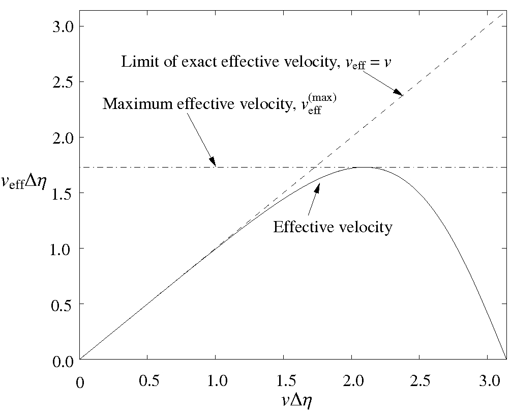
Figure 6: The effective particle velocities produced by the 4th-order compact Padé difference scheme in $\eta$ space. After Eliasson (2006).

In order to investigate the impact of the difference scheme in the Fourier transformed velocity space on effective particle velocities, we study an approximation of the Fourier transformed Vlasov equation, in which the $x$ and $t$ derivatives are performed exactly, while the $\eta$ derivative is approximated by Eq. (89). The difference scheme can formally be written as a difference operator $D_{\eta}$, giving rise to the difference-differential equation

$$\frac{\partial\widehat{f}}{\partial t}-\mathrm{i}\frac{\partial}{\partial x}(D_{\eta}\widehat{f})+\mathrm{i}E\eta\widehat{f}=0$$ (95)

In order to study the effect of the difference approximation $D_{\eta}$ on the solution in $v$ space, the definition (51) is inserted into Eq. (95), giving

$$\frac{1}{2\pi}\int_{-\infty}^{\infty}\bigg{[}\frac{\partial f}{\partial t}e^{\mathrm{i}\eta v}-\mathrm{i}\frac{\partial f}{\partial x}D_{\eta}(e^{\mathrm{i}\eta v})+\mathrm{i}E\eta fe^{\mathrm{i}\eta v}\bigg{]}\,\mathrm{d}v=0$$ (96)

where the difference operator gives $D_{\eta}(e^{\mathrm{i}\eta v})=\mathrm{i}v_{\mathrm{eff}}(v)e^{\mathrm{i}\eta v}$ with the effective particle velocity $\mathrm{i}v_{\mathrm{eff}}(v)$, and the term $\mathrm{i}E\eta fe^{\mathrm{i}\eta v}$ gives rise to the term $-e^{\mathrm{i}E\eta v}\partial f/\partial v$ by an integration by parts, yielding

$$\frac{1}{2\pi}\int_{-\infty}^{\infty}\bigg{[}\frac{\partial f}{\partial t}+v_{\mathrm{eff}}(v)\frac{\partial f}{\partial x}-E\frac{\partial f}{\partial v}\bigg{]}e^{\mathrm{i}\eta v}\,\mathrm{d}v=0,$$ (97)

and thus

$$\frac{\partial f}{\partial t}+v_{\mathrm{eff}}(v)\frac{\partial f}{\partial x}-E\frac{\partial f}{\partial v}=0,$$ (98)

which is an approximation of the Vlasov equation (44), with the effective velocity $v_{\mathrm{eff}}(v)$ produced by the numerical differentiation in $\eta$ space. For the Padé scheme (89) we have

$$v_{\mathrm{eff}}(v)=\frac{3}{\Delta\eta}\frac{\sin(v\Delta\eta)}{[2+\cos(v\Delta\eta)]}.$$ (99)

In the limit $v\Delta\eta\rightarrow 0$, then $v_{\mathrm{eff}}\rightarrow v$; see Fig. 6 where $v_{\mathrm{eff}}\Delta\eta$ has been plotted as a function of $v\Delta\eta$. The equations for the particle trajectories in $(x,v)$ space, produced by Eq. (98), are

$$\dot{x}(t) =v_{\mathrm{eff}}[v(t)]=\frac{3}{\Delta\eta}\frac{\sin[v(t)\Delta\eta]}{\{2+\cos[v(t)\Delta\eta]\}}$$ (100)

$$\dot{v}(t) =-\frac{e}{m_{\mathrm{e}}}E[x(t),t],$$ (101)

where the dots in the left-hand sides denote time derivatives $d/dt$. Thus the particles are transported in $x$ space with the effective velocity $v_{\mathrm{eff}}$, which is periodic in $v$. If the product $v\Delta\eta$ is too large, then the approximation $v_{\mathrm{eff}}\approx v$ breaks down; see Fig. 6. A maximum effective velocity, $v_{\mathrm{eff}}^{(\mathrm{max})}\Delta\eta=\sqrt{3}\approx 1.73$, can be found for $v\Delta\eta=2\pi/3\approx 2.09$. It means that even though the largest represented velocity is given by the Nyquist limit $v_{\mathrm{max}}=\pi/\Delta\eta\approx 3.14/\Delta\eta$, the highest effective velocity for transport of particles in $x$ space is $v_{\mathrm{eff}}^{(\mathrm{max})}=\sqrt{3}/\Delta\eta$. In numerical experiments, one has to choose a small enough $\Delta\eta$, so that important phenomena in velocity space, for example beams of particles, are well resolved, i.e., the velocities of these particles must fulfil $v<v_{\mathrm{eff}}^{(\mathrm{max})}$ with some margin. In the simulation performed to produce the results in the present section, particles were accelerated to velocities somewhat less than $v=5$; see the left-hand panel of Fig. 3. The grid size was $\Delta\eta=(120/600)=0.2$, which gives that $v\Delta\eta\approx 1.0$ for these particles. According to the diagram in Fig. 6, the effective velocity is close to the limit of exact velocity for the value $v\Delta\eta=1.0$, and thus the particle velocities for the fastest particles are well resolved. The maximum effective velocity produced in the simulation was $v_{\mathrm{eff}}^{(\mathrm{max})}=\sqrt{3}/\Delta\eta\approx 8.6$.

IV.3 The choice of domain and grid sizes

When using the numerical algorithm to solve physical problems, it is important to know what is the computational domain and resolution in the real velocity space, i.e., what is the maximum velocity component $v_{{\rm max}}$, used in the real velocity space to resolve the particle distribution function and what is the grid size $\Delta v$ used in the numerical solution. For given $\eta_{{\rm max}}$ and $\Delta\eta$, the maximum represented velocity and the grid size in velocity space are given by

$$v_{{\rm max}}=\frac{\pi}{\Delta\eta}$$ (102)

and

$$\Delta v=\frac{\pi}{\eta_{{\rm max}}},$$ (103)

respectively. In view of the results in Fig. 6, one should choose $\Delta\eta$ small enough such that the maximum velocity component $v_{{\rm max}}$ is more than twice the maximum particle velocity one wants to resolve in the numerical solution, in order to avoid dispersive errors on the particle velocities. One must also choose ${\eta_{{\rm max}}}$ large enough so that fine enough structures in the velocity distribution function is resolved.

IV.4 One-dimensional simulations of electron and ion holes

In simulations of processes with several timescales, it is important that the numerical scheme does not introduce artificial heating of the electrons. Such effects can be a problem if a diffusion operator is introduced in velocity space to minimize the filamentation effects in the Vlasov equation. In the Fourier method used here, there is minimal heating effects of the electrons since only the highest Fourier modes in velocity space are absorbed by the outflow boundary condition in the Fourier transformed velocity space. As examples we will study the dynamics of electron and ion holes in an electron-ion plasma, which is governed by the Vlasov-Poisson system of equations for electrons and ions,

$$\frac{\partial f_{e}}{\partial t}+v\frac{\partial f_{e}}{\partial x}+\frac{e}{m_{e}}\frac{\partial\Phi}{\partial x}\frac{\partial f_{e}}{\partial v}=0,$$ (104)

$$\frac{\partial f_{i}}{\partial t}+v\frac{\partial f_{i}}{\partial x}-\frac{e}{m_{i}}\frac{\partial\Phi}{\partial x}\frac{\partial f_{i}}{\partial v}=0,$$ (105)

$$-\frac{\partial^{2}\Phi}{\partial x^{2}}=\frac{e}{\varepsilon_{0}}\bigg{[}\int_{-\infty}^{\infty}(f_{i}(x,v,t)-f_{e}(x,v,t))\,\mathrm{d}v\bigg{]},$$ (106)

and where both the electron and ion dynamics are important. As initial conditions for the simulations, we have used Schamel’s quasi-stationary solutions for electron and ion holes (Schamel, 1979, 1971; Bujarbarua and Schamel, 1981; Schamel, 1986).

Figure 7: The electron distribution function for two electron holes at time $t=0$ (upper left panel), $t=155\,\omega_{pe}^{-1}$ (upper right panel), $t=175\,\omega_{pe}^{-1}$ (middle left panel), $t=251\,\omega_{pe}^{-1}$ (middle right panel), $t=461\,\omega_{pe}^{-1}$ (lower left panel) and $t=576$ (lower right panel). The color bars go from dark blue (small values) to dark red (large values). After Eliasson and Shukla (2004a).

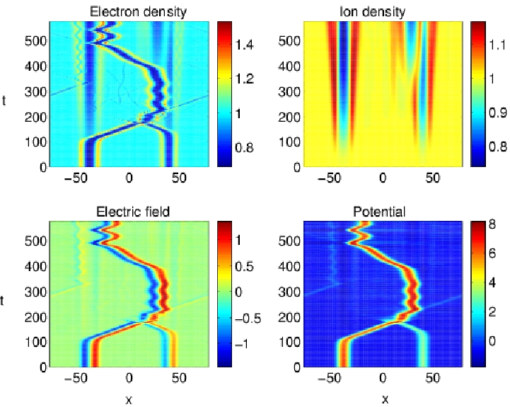
Figure 8: The time and space evolution of the electron density (upper left panel), the ion density (upper right panel), the electric field (lower left panel) and the potential (lower right panel) associated with the two electron holes in Fig. 7. After Eliasson and Shukla (2004a).

Figures 8 and 7 show a simulation of interacting electron holes in and electron-ion plasma with mobile ions and realistic ion to electron mass ratio of 29500 for oxygen ions (Eliasson and Shukla, 2004a). Two large-amplitude electron holes were initially placed at $x=-40\,r_{De}$ and $x=40\,r_{De}$, displayed at $t=0$ in the phase space number density plots in Fig. 7 (top left panel). A small electron density perturbation, centered at the two electron holes, were introduced as a seed for any instability. The ion density was initially taken to be homogeneous. We see in Fig. 7 that at $t=155\,\omega_{pe}^{-1}$ (top right panel), the two electron holes having started moving towards each other, and that at $t=175\,\omega_{pe}^{-1}$ they are colliding and are merging to a new electron hole (middle left panel), and that the newly created electron hole at $t=461\,\omega_{pe}^{-1}$ has propagated to $x=30\,r_{De}$ (middle right panel), and at a later stage it has propagated to $x=-30\,r_{De}$ where it remains throughout the simulation (lower panels). The reason for this complicated behavior of the electron holes can be understood by studying the interaction with the ions in detail. Due to their positive potential, the electron holes expel the ions and create local ion density cavities, which in turn eject and accelerate the electron holes. This can clearly be seen in Fig. 8, where the two electron holes start propagating at $t\approx 100\,\omega_{pe}^{-1}$ and $t\approx 130\,\omega_{pe}^{-1}$, respectively. At $t\approx 170\,\omega_{pe}^{-1}$, the two electron holes collide and merge into a new electron hole with larger amplitude, which propagates slightly in the positive $x$ direction, and becomes trapped at a local ion density maximum at $x\approx 30\,r_{De}$; see the upper right panel of Fig. 8 for the ion density and the lower right panel for the potential. After $t\approx 400\,\omega_{pe}^{-1}$, a new ion density cavity is created where the electron hole is centered, and at this time the electron hole is again ejected and accelerated in the negative $x$ direction. At $t\approx 480\,\omega_{pe}^{-1}$, the moving electron hole again encounters an ion density maximum located at $x\approx-30\,r_{De}$, where it is again trapped, performing large oscillations. We see that the electron holes remain stable during the acceleration by ion density cavities and survive on an ion time scale, much longer than the electron plasma period.

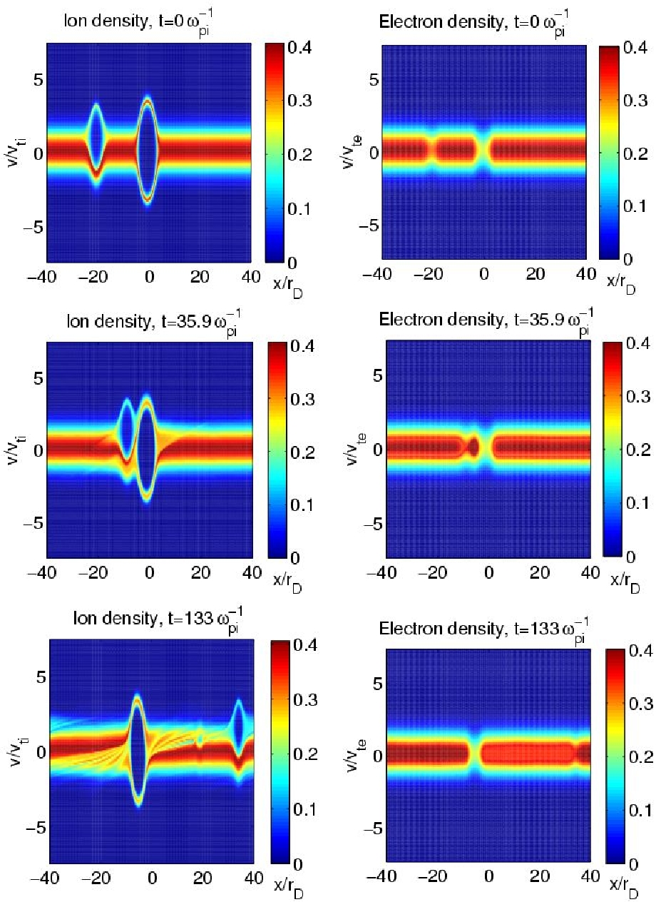
Figure 9: The distribution function for the ions (left panels) and electrons (right panels) of two colliding ion holes, before the collision at times $t=0\,\omega_{pi}$ (upper panel) and $t=35.9\,\omega_{pi}$ (middle panel), and after the collision at $t=133\,\omega_{pi}$ (lower panel). The color bars go from dark blue (small values) to dark red (large values). After Eliasson and Shukla (2004b).

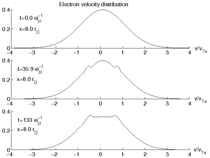
Figure 10: The electron velocity distribution at $x=8\,r_{D}$, for $t=0\,\omega_{pi}^{-1}$ (upper panel), $t=35.9\,\omega_{pi}^{-1}$ (middle panel) and $t=133\,\omega_{pi}^{-1}$ (lower panel). After Eliasson and Shukla (2004b).

Figure 9 displays the features of the ion and electron distribution functions for two colliding ion holes, where initially (upper panels) the left ion hole propagates with the speed $u_{0}=0.9\,v_{Ti}$ where $v_{Ti}=\sqrt{k_{B}T_{i}/m_{i}}$ is the ion thermal speed, and the right ion hole is standing. The ion and electron distribution functions associated with the ion holes are shown before collision at times $t=0\,\omega_{pi}^{-1}$ (upper panels) and $t=35.9\,\omega_{pi}^{-1}$ (middle panels), and after collision at time $t=133\,\omega_{pi}^{-1}$ (lower panels), where $\omega_{pi}=(n_{0}e^{2}/\varepsilon_{0}m_{i})^{1/2}$ is the ion plasma frequency. Figure 9 exhibits that the ion holes undergo collisions without being destroyed; thus they are robust structures. As can be seen in the right panels of Fig 9, the electrons have a non-Maxwellian, flat topped distribution in the region between the ion holes after collision has taken place. The velocity distribution function is plotted as a function of $v/v_{Te}$ in Fig. 10 at $x=8.0\,r_{De}$. We see that the initial Maxwellian distribution (the upper panel) changes to a distribution with beams at $v\approx\pm 0.6\,v_{Te}$ (the middle panel) slightly before collision, and to a flat-top distribution with two maxima after collision (the lower panel). The reason for this phenomenon is that the two ion holes are associated with negative electrostatic potentials, and the electrons entering the region between the ion holes after collision must have a large enough kinetic energy to cross the potential barriers that are set up by the ion holes. Therefore, the region between the ion holes becomes excavated of low energy electrons. Also here the features of the electron distribution function survives on the ion time-scale, much longer than the electron plasma period.

V The two-dimensional Vlasov equation

We here discuss the extension of the Fourier transform method to the Fourier transformed Vlasov equation in two spatial and two velocity dimensions, including external and self-consistent magnetic fields. In the design of well-posed absorbing boundary conditions in the Fourier transformed velocity space, special care has to be taken with the magnetic field, which enters into the formulation of the boundary condition.

V.1 The two-dimensional Vlasov-Poisson system

The two-dimensional Vlasov-Poisson system for electrons reads

$$\frac{\partial f}{\partial t}+v_{1}\frac{\partial f}{\partial x_{1}}+v_{2}\frac{\partial f}{\partial x_{2}}-\frac{e}{m}\left(E_{1}\frac{\partial f}{\partial v_{1}}+E_{2}\frac{\partial f}{\partial v_{2}}+Bv_{2}\frac{\partial f}{\partial v_{1}}-Bv_{1}\frac{\partial f}{\partial v_{2}}\right)=0$$ (107)

$$E_{1}=-\frac{\partial\Phi}{\partial x_{1}},\qquad E_{2}=-\frac{\partial\Phi}{\partial x_{2}}$$ (108)

$$-\left(\frac{\partial^{2}\Phi}{\partial x_{1}^{2}}+\frac{\partial^{2}\Phi}{\partial x_{2}^{2}}\right)=\frac{e}{\varepsilon_{0}}\left[n_{0}-\int_{-\infty}^{\infty}\int_{-\infty}^{\infty}f\,\mathrm{d}v_{1}\,\mathrm{d}v_{2}\right]$$ (109)

where $n_{0}$ is the neutralizing heavy ion density background, fixed uniformly in space. The external magnetic field ${\bf B}(x_{1},x_{2},t)$ is here directed along the $x_{3}$ axis, perpendicular to the $(x_{1},x_{2})$ plane, and the electrostatic potential is calculated self-consistently from Poisson’s equation.

By using the Fourier transform pair

$$f(x_{1},x_{2},v_{1},v_{2},t) =\int_{-\infty}^{\infty}\int_{-\infty}^{\infty}\widehat{f}(x_{1},x_{2},\eta_{1},\eta_{2},t)\mathrm{e}^{-\mathrm{i}(\eta_{1}v_{1}+\eta_{2}v_{2})}\,\mathrm{d}\eta_{2}\,\mathrm{d}\eta_{1}$$

$$\widehat{f}(x_{1},x_{2},\eta_{1},\eta_{2},t) =\frac{1}{(2\pi)^{2}}\int_{-\infty}^{\infty}\int_{-\infty}^{\infty}f(x_{1},x_{2},v_{1},v_{2},t)e^{\mathrm{i}(\eta_{1}v_{1}+\eta_{2}v_{2})}\,\mathrm{d}v_{2}\,\mathrm{d}v_{1}$$ (110)

the system (107)–(109) is transformed into

$$\frac{\partial\widehat{f}}{\partial t}-\mathrm{i}\frac{\partial^{2}\widehat{f}}{\partial x_{1}\partial\eta_{1}}-\mathrm{i}\frac{\partial^{2}\widehat{f}}{\partial x_{2}\partial\eta_{2}}+\frac{e}{m}\bigg{[}\mathrm{i}(E_{1}\eta_{1}+E_{2}\eta_{2})\widehat{f}+B\eta_{1}\frac{\partial\widehat{f}}{\partial\eta_{2}}-B\eta_{2}\frac{\partial\widehat{f}}{\partial\eta_{1}}\bigg{]}=0,$$ (111)

$$E_{1}=-\frac{\partial\Phi}{\partial x_{1}},\qquad E_{2}=-\frac{\partial\Phi}{\partial x_{2}},$$ (112)

$$-\left(\frac{\partial^{2}\Phi}{\partial x_{1}^{2}}+\frac{\partial^{2}\Phi}{\partial x_{2}^{2}}\right)=\frac{e}{\varepsilon_{0}}\left[n_{0}-(2\pi)^{2}\widehat{f}_{\eta_{1}=\eta_{2}=0}\right].$$ (113)

The systems (107)–(109) and (111)–(113) can be cast into dimensionless form

$$\frac{\partial f}{\partial t}+v_{1}\frac{\partial f}{\partial x_{1}}+v_{2}\frac{\partial f}{\partial x_{2}}-\left(E_{1}\frac{\partial f}{\partial v_{1}}+E_{2}\frac{\partial f}{\partial v_{2}}+Bv_{2}\frac{\partial f}{\partial v_{1}}-Bv_{1}\frac{\partial f}{\partial v_{2}}\right)=0,$$ (114)

$$E_{1}=-\frac{\partial\Phi}{\partial x_{1}},\qquad E_{2}=-\frac{\partial\Phi}{\partial x_{2}}$$ (115)

$$-\left(\frac{\partial^{2}\Phi}{\partial x_{1}^{2}}+\frac{\partial^{2}\Phi}{\partial x_{2}^{2}}\right)=1-\int_{-\infty}^{\infty}\int_{-\infty}^{\infty}f\,\mathrm{d}v_{1}\,\mathrm{d}v_{2}$$ (116)

and

$$\frac{\partial\widehat{f}}{\partial t}-\mathrm{i}\frac{\partial^{2}\widehat{f}}{\partial x_{1}\partial\eta_{1}}-\mathrm{i}\frac{\partial^{2}\widehat{f}}{\partial x_{2}\partial\eta_{2}}+\mathrm{i}(E_{1}\eta_{1}+E_{2}\eta_{2})\widehat{f}+B\eta_{1}\frac{\partial\widehat{f}}{\partial\eta_{2}}-B\eta_{2}\frac{\partial\widehat{f}}{\partial\eta_{1}}=0$$ (117)

$$E_{1}=-\frac{\partial\Phi}{\partial x_{1}},\qquad E_{2}=-\frac{\partial\Phi}{\partial x_{2}}$$ (118)

$$-\left(\frac{\partial^{2}\Phi}{\partial x_{1}^{2}}+\frac{\partial^{2}\Phi}{\partial x_{2}^{2}}\right)=1-(2\pi)^{2}\widehat{f}_{\eta_{1}=\eta_{2}=0}$$ (119)

respectively, where time $t$ has been normalized by $\omega_{\mathrm{pe}}^{-1}$, the velocity variables $v_{1}$ and $v_{2}$ by $v_{\mathrm{th,e}}$, the Fourier transformed velocity variables $\eta_{1}$ and $\eta_{2}$ by $v_{\mathrm{th,e}}^{-1}$, the spatial variables $x_{1}$ and $x_{2}$ by $r_{\mathrm{De}}$, the Fourier transformed distribution function $\widehat{f}$ by $n_{0}$, the function $f$ by $n_{0}v_{\mathrm{th,e}}^{-2}$, the electric field components $E_{1}$ and $E_{2}$ by $v_{\mathrm{th,e}}^{2}r_{\mathrm{De}}^{-1}m_{e}/e$, the electric potential $\Phi$ by $v_{\mathrm{th,e}}^{2}(m/e)$, and the magnetic field $B$ by $\omega_{\rm pe}m_{\rm e}/e$.

In order to adapt the system (117)–(119) for numerical simulations, the computational domain is restricted to ${0\leq x_{1}<L_{1}}$, ${0\leq x_{2}<L_{2}}$, $0\leq\eta_{1}\leq\eta_{{\rm max},1}$ and $-\eta_{{\rm max},2}\leq\eta_{2}\leq\eta_{{\rm max},2}$. For negative $\eta_{1}$, the symmetry $\widehat{f}(x_{1},x_{2},\eta_{1},\eta_{2},t)=\widehat{f}^{*}(x_{1},x_{2},-\eta_{1},-\eta_{2},t)$ is used to obtain function values, if needed, owing to that the original distribution function $f(\textbf{x},\textbf{v},t)$ is real-valued. It is therefore not necessary to represent the solution for negative $\eta_{1}$ on the numerical grid. In the $x_{1}$ and $x_{2}$ directions, the periodic boundary conditions

$$\widehat{f}(x_{1}+L_{1},x_{2},\eta_{1},\eta_{2},t) =\widehat{f}(x_{1},x_{2},\eta_{1},\eta_{2},t)$$ (120)

and

$$\widehat{f}(x_{1},x_{2}+L_{2},\eta_{1},\eta_{2},t) =\widehat{f}(x_{1},x_{2},\eta_{1},\eta_{2},t)$$ (121)

respectively, are used.

V.2 Outflow boundary conditions in Fourier transformed velocity space

Similar to the one-dimensional Vlasov-Poisson system discussed above, we wish to design absorbing artificial boundary conditions in the Fourier transformed velocity space, so that the highest oscillations in velocity space can be captured at the boundary and removed from the calculation. Hence, at the boundaries at $\eta_{1}=\eta_{{\rm max},1}$ and $\eta_{2}=\pm\eta_{{\rm max},2}$, the strategy is to let outgoing waves pass over the boundaries, and to set incoming waves to zero. We explore the idea by studying the reduced initial value problem with only a constant magnetic field ${B=B_{0}}$,

$$\frac{\partial\widehat{f}}{\partial t}-\mathrm{i}\frac{\partial^{2}\widehat{f}}{\partial x_{1}\partial\eta_{1}}-\mathrm{i}\frac{\partial^{2}\widehat{f}}{\partial x_{2}\partial\eta_{2}}+B_{0}\eta_{1}\frac{\partial\widehat{f}}{\partial\eta_{2}}-B_{0}\eta_{2}\frac{\partial\widehat{f}}{\partial\eta_{1}}=0$$ (122)

$$f(x_{1},x_{2},\eta_{1},\eta_{2},0)=f_{0}(x_{1},x_{2},\eta_{1},\eta_{2})$$ (123)

A Fourier transform in space ($\partial/\partial x_{1}\rightarrow ik_{x1}$ and $\partial/\partial x_{2}\rightarrow ik_{x2}$) gives a new differential equation for the unknown function $\widetilde{f}(k_{x1},k_{x2},\eta_{1},\eta_{2},t)$,

$$\frac{\partial\widetilde{f}}{\partial t}+(k_{x1}-B_{0}\eta_{2})\frac{\partial\widetilde{f}}{\partial\eta_{1}}+(k_{x2}+B_{0}\eta_{1})\frac{\partial\widetilde{f}}{\partial\eta_{2}}=0$$ (124)

$$\widetilde{f}(k_{x1},k_{x2},\eta_{1},\eta_{2},t)_{t=0}=\widetilde{f}_{0}(k_{x1},k_{x2},\eta_{1},\eta_{2})$$ (125)

This is a hyperbolic equation for which the initial values are transported along the characteristic curves, given by

$$\frac{\mathrm{d}\eta_{1}(t)}{\mathrm{d}t} =k_{x1}-B_{0}\eta_{2}(t)$$ (126)

$$\frac{\mathrm{d}\eta_{2}(t)}{\mathrm{d}t} =k_{x2}-B_{0}\eta_{1}(t)$$ (127)

Along the boundary $\eta_{1}=\eta_{{\rm max},1}$, Eq. (126) describes an outflow of data when ${k_{x1}-B_{0}\eta_{2}\geq 0}$ and an inflow of data when $k_{x1}-B_{0}\eta_{2}<0$. A well-posed boundary condition is to set the inflow to zero at the boundary, i.e.,

$$\widetilde{f}_{\eta_{1}=\eta_{{\rm max},1}}=0,\hskip 14.22636ptk_{x1}-B_{0}\eta_{2}<0$$ (128)

which can be expressed with the help of the Heaviside step function $H$ as

$$\widetilde{f}=H(k_{x1}-B_{0}\eta_{2})\widetilde{f},\hskip 14.22636pt\eta_{1}=\eta_{{\rm max},1}$$ (129)

where

$$H(k_{x1}-B_{0}\eta_{2})=\left\{\begin{array}[]{l}1,\hskip 14.22636ptk_{x1}-B_{0}\eta_{2}\geq 0\\ 0,\hskip 14.22636ptk_{x1}-B_{0}\eta_{2}<0\end{array}\right.$$ (130)

The boundary condition (129) allows outgoing waves to pass over the boundary and to be removed, while incoming waves are set to zero; the removal of the outgoing waves corresponds to the losing of information about the finest structures in velocity space.

Inverse Fourier transforming Eq. (130) then gives the boundary condition for the original problem (122) as

$$\widehat{f}=\mathrm{F}_{1}^{-1}H(k_{x1}-B_{0}\eta_{2})\mathrm{F}_{1}\widehat{f},\hskip 14.22636pt\eta_{1}=\eta_{{\rm max},1}$$ (131)

The operator $\mathrm{F}_{1}^{-1}H(k_{x1}-B_{0}\eta_{2})\mathrm{F}_{1}$ is a projection operator which removes incoming waves at the boundary ${\eta_{1}=\eta_{{\rm max},1}}$. Similarly, the boundary conditions at $\eta_{2}=\pm\eta_{{\rm max},2}$ becomes

$$\widehat{f} =\mathrm{F}_{2}^{-1}H(k_{x2}+B_{0}\eta_{1})\mathrm{F}_{2}\widehat{f},\hskip 14.22636pt\eta_{2}=\eta_{{\rm max},2}$$ (132)

and

$$\widehat{f} =\mathrm{F}_{2}^{-1}H(-k_{x2}-B_{0}\eta_{1})\mathrm{F}_{2}\widehat{f},\hskip 14.22636pt\eta_{2}=-\eta_{{\rm max},2}$$ (133)

respectively.

In order to find well-posed boundary conditions in the $\eta_{1}$ and $\eta_{2}$ directions in the case when $B=B(x_{1},x_{2},t)$ varies in time $t$ and in the $x_{1}$ and $x_{2}$ space with the periodicities $L_{1}$ and $L_{2}$, respectively, Eq. (117) is rewritten in an equivalent form as

$$\begin{split}\frac{\partial\widehat{f}}{\partial t}-\mathrm{i}\theta_{1}\frac{\partial}{\partial\eta_{1}}\left(\frac{\partial}{\partial x_{1}}-\mathrm{i}\eta_{2}B_{01}\right)(\widehat{f}\theta_{1}^{-1})-\mathrm{i}\theta_{2}\frac{\partial}{\partial\eta_{2}}\left(\frac{\partial}{\partial x_{2}}+\mathrm{i}\eta_{1}B_{02}\right)(\widehat{f}\theta_{2}^{-1})+\mathrm{i}(E_{1}\eta_{1}+E_{2}\eta_{2})\widehat{f}=0\end{split}$$ (134)

where we introduced the spatially averaged magnetic fields

$$B_{01}(x_{2},t)=\frac{1}{L_{1}}\int_{0}^{L_{1}}B\,\mathrm{d}x_{1},\qquad B_{02}(x_{1},t)=\frac{1}{L_{2}}\int_{0}^{L_{2}}B\,\mathrm{d}x_{2}$$ (135)

and the phase factors

$$\theta_{1}=\exp\bigg{[}\mathrm{i}\eta_{2}\int_{0}^{x_{1}}(B-B_{01})\,\mathrm{d}x_{1}\bigg{]},\qquad\theta_{2}=\exp\bigg{[}-\mathrm{i}\eta_{1}\int_{0}^{x_{2}}(B-B_{02})\,\mathrm{d}x_{2}\bigg{]}.$$ (136)

We note that if $B$ is periodic and continuous in the $x_{1}$ and $x_{2}$ directions, then the integrals $\int_{0}^{x_{1}}(B-B_{01})\mathrm{d}x_{1}$ and $\int_{0}^{x_{2}}(B-B_{02})\mathrm{d}x_{2}$ are also periodic and continuous functions, and the $x_{1}$ and $x_{2}$ derivatives can be approximated accurately by using the pseudo-spectral method.

By studying the flow of data in the $\eta_{1}$ direction for the function $\phi_{1}=\widehat{f}\theta_{1}^{-1}$ and the flow of data in the $\eta_{2}$ direction for the function $\phi_{2}=\widehat{f}\theta_{2}^{-1}$, one can find outflow boundary condition in the $\eta_{1}$ and $\eta_{2}$ directions, similar to the conditions (131)–(133), as

$$\begin{split}\widehat{f}&=\theta_{1}\mathrm{F}_{1}^{-1}H(k_{x1}-\eta_{2}B_{01})\mathrm{F}_{1}(\widehat{f}\theta_{1}^{-1}),\hskip 14.22636pt\eta_{1}=\eta_{{\rm max},1}\end{split}$$ (137)

$$\begin{split}\widehat{f}&=\theta_{2}\mathrm{F}_{2}^{-1}H(k_{x2}+\eta_{1}B_{02})\mathrm{F}_{2}(\widehat{f}\theta_{2}^{-1}),\hskip 14.22636pt\eta_{2}=\eta_{{\rm max},2}\end{split}$$ (138)

$$\begin{split}\widehat{f}&=\theta_{2}\mathrm{F}_{2}^{-1}H(-k_{x2}-\eta_{1}B_{02})\mathrm{F}_{2}(\widehat{f}\theta_{2}^{-1}),\hskip 14.22636pt\eta_{2}=-\eta_{{\rm max},2}\end{split}$$ (139)

respectively. In the case when $B$ is independent of $x_{1}$ and $x_{2}$, the boundary conditions (137)–(139) reduce to the conditions (131)–(133). The boundary operators are projection operators, which allow outgoing waves to pass over the $\boldsymbol{\eta}$ boundaries of the domain and to be removed from the domain, while incoming waves are set to zero. The well-posedness of these boundary conditions was proven by showing that a positive definite energy integral is non-increasing in time (Eliasson, 2002).

V.3 Electron Bernstein and upper hybrid waves in magnetized plasmas

We will here give examples of some effects related to linear electron oscillations in magnetized plasmas. These include electron Bernstein modes that are exactly undamped according to Landau theory. Due to this fact, there is a recurrence effect in a weakly magnetized plasma, namely, there appears that waves can be periodically Landau damped only to recur in the plasma at a later time. We here compare simulation results with linear theory, in the form of dispersion corves for Bernstein mode waves and time-dependent analytic solutions of the Vlasov equation for a magnetized electron-ion plasma with immobile ions.

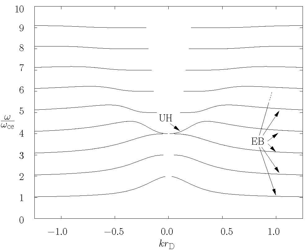
(a) Dispersion diagram

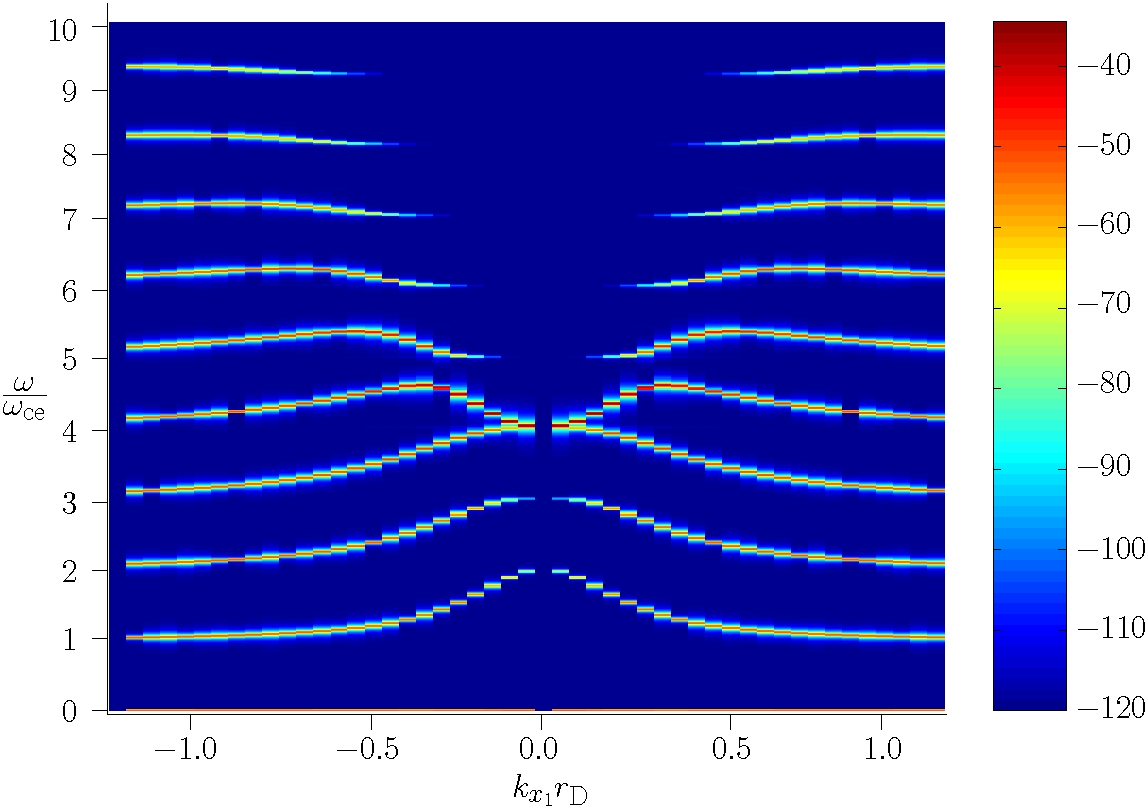
(b) Power spectrum

Figure 11: Dispersion diagram and power spectrum (decibel) for electrostatic electron Bernstein (EB) and upper hybrid (UH) waves; $\omega_{\mathrm{uh}}=4\omega_{\mathrm{ce}}$. After Eliasson (2008).

The dispersion relation for the linear upper hybrid and electron Bernstein modes in a Maxwellian plasma is given by Crawford and Tataronis (1965) as

$$1+\bigg{(}\frac{\omega_{\mathrm{pe}}}{\omega_{\mathrm{ce}}}\bigg{)}^{2}\exp(-\lambda)\int_{\psi=0}^{\pi}\frac{\sin(\psi\omega^{\prime})\sin(\psi)\exp[-\lambda\cos(\psi)]}{\sin(\pi\omega^{\prime})}\mathrm{d}\psi =0$$ (140)

where

$$\omega^{\prime} =\omega/\omega_{\mathrm{ce}},$$ (141)

$$\lambda =(kr_{\mathrm{D}})^{2}\bigg{(}\frac{\omega_{\mathrm{pe}}}{\omega_{\mathrm{ce}}}\bigg{)}^{2},$$ (142)

$$k^{2} =k_{x1}^{2}+k_{x2}^{2}.$$ (143)

Solving for $\omega^{\prime}$ in Eq. (140) gives the relation between $\omega$ and $k$. Figure  11(a) shows the dispersion curves for the case $\omega_{\mathrm{uh}}=4\omega_{\mathrm{ce}}$, and Fig. 11(b) shows the power spectrum in space and time from a simulation of the Vlasov equation with the same parameters. In the simulation, the obtained time series of the electric field component $E_{1}$ was Fourier transformed in $x_{1}$ space and in time (using a Hamming window), to produce a power spectrum in a logarithmic scale.

As can be seen in Fig. 11(b), the electrostatic energy is concentrated at the linear Bernstein eigen-modes, in good agreement with theory. In the long wavelength limit $kr_{D}\ll 1$, Eq. (140) reduces to the dispersion relation

$$\omega^{2}=\omega_{\mathrm{uh}}^{2}+\frac{3v_{\mathrm{th,e}}^{2}k^{2}}{\omega^{2}-3\omega_{ce}^{2}}$$ (144)

where $\omega_{\mathrm{uh}}=(\omega_{\mathrm{pe}}^{2}+\omega_{\mathrm{ce}}^{2})^{1/2}$ is the upper hybrid frequency. However, taking electromagnetic effects into account, there are corrections in the long wavelength limit where the upper hybrid waves go over to the electromagnetic $Z$ mode waves which we will discuss below. A zero-frequency ($\omega=0$) mode, which is not a solution of the dispersion relation (140), can be seen in the power spectrum in Fig. 11(b); this “convective mode” has earlier been observed in numerical PIC simulations by Kamimura et al. (1978), and theoretically by Sukhorukov and Stubbe (1997). In terms of Landau theory, this mode is related to a pole in the initial condition, and not to a solution of the dispersion relation (140).

The simulation was restricted to one spatial dimension, along the $x_{1}$ axis, where the simulation domain was set to ${0\leq x_{1}/r_{\mathrm{D}}\leq 40\pi}$, ${0\leq\eta_{1}v_{\mathrm{th,e}}\leq 15}$ and ${0\leq\eta_{2}v_{\mathrm{th,e}}\leq 15}$ and the number of intervals ${N_{x1}=50}$, ${N_{\eta_{1}}=60}$ and ${2N_{\eta_{2}}=120}$, respectively. The initial condition was set to

$$\widehat{f}(x_{1},x_{2},\eta_{1},\eta_{2},0)=n(x_{1})\widehat{f}_{0}(\eta_{1},\eta_{2})$$ (145)

where the perturbed relative density was set to a sum of waves with all possible wavenumbers,

$$n(x_{1})=\bigg{[}1+A\sum_{i_{1}=1}^{24}i_{1}\sin(0.05i_{1}x_{1}/r_{\mathrm{D}})\bigg{]}$$ (146)

with the amplitude set to $A=0.0001$, giving an almost linear problem. The Fourier transformed velocity distribution was set to a Maxwellian,

$$\widehat{f}_{0}(\eta_{1},\eta_{2}) =\frac{n_{0}}{(2\pi)^{2}}\exp\bigg{[}-\frac{1}{2}(\eta_{1}^{2}+\eta_{2}^{2})v_{\mathrm{th,e}}^{2}\bigg{]}$$ (147)

In velocity v space, the Maxwellian would be

$$f_{0}(v_{1},v_{2}) =\frac{n_{0}}{v_{\mathrm{th,e}}^{2}}\frac{1}{2\pi}\exp\bigg{[}-\frac{1}{2v_{\mathrm{th,e}}^{2}}(v_{1}^{2}+v_{2}^{2})\bigg{]}$$ (148)

The external magnetic field was kept constant in the simulation, with the ratio $\omega_{\mathrm{pe}}/\omega_{\mathrm{ce}}=\sqrt{15}$ (giving $\omega_{\mathrm{uh}}=4\omega_{\mathrm{ce}}$). The number of time steps taken was $N_{t}=42\,530$ and the end time $t_{\mathrm{end}}=1737\omega_{\mathrm{pe}}^{-1}$ with a fixed timestep.

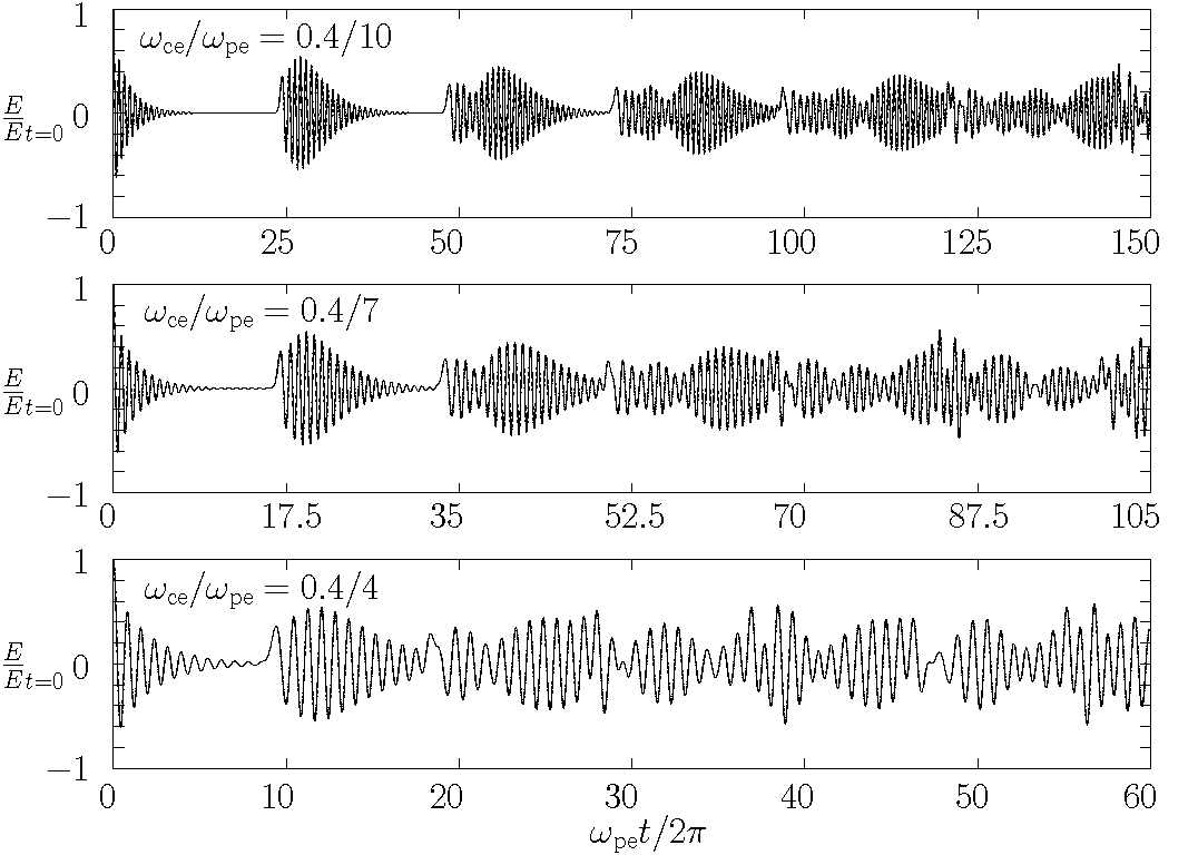
(a) Simulation results

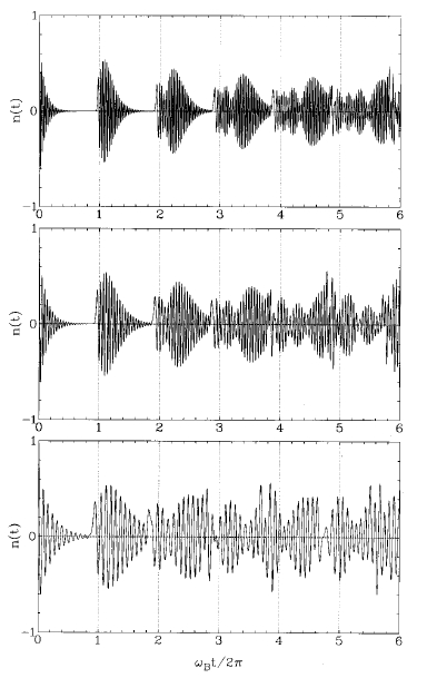
(b) Analytic solutions

Figure 12: Pseudo-periodically damping and recurrence of electrostatic waves propagating perpendicularly to the magnetic field in a weakly magnetized plasma; the so-called Bernstein-Landau paradox. (a): Simulation results for different magnetic fields. (b): Analytic solutions by Sukhorukov and Stubbe (1997).

According to linear theory, wave solutions of the unmagnetized Vlasov equation exhibit collision-less damping, while in magnetized plasma waves propagating perpendicularly to the magnetic field ${\bf B}_{\mathrm{ext}}$ are exactly undamped, no matter how weak the magnetic field is. This is the so-called Bernstein-Landau paradox; it seems that the theory for magnetized plasma does not converge smoothly to the theory for unmagnetized plasma when the magnetic field strength decreases.

This problem was investigated theoretically by Sukhorukov and Stubbe (1997) who derived analytical solutions of the problem. In Fig. 12, we have compared a numerical solution of the Vlasov equation with the analytic solution of Sukhorukov and Stubbe (1997) for a wave with the wavenumber $k_{x}=0.4\,r_{\mathrm{D}}^{-1}$ and with different values on the magnetic field, such that $\omega_{\mathrm{ce}}/\omega_{\mathrm{pe}}=0.4/10$, $0.4/7$ and $0.4/4$, where $\omega_{\mathrm{ce}}=eB_{\mathrm{ext}}/m_{\mathrm{e}}$. The numerical result obtained from the Vlasov simulation can be seen in Fig. 12(a) show excellent agreement with the analytic results of Sukhorukov and Stubbe (1997) in Fig. 12(b). For the numerical results, where the electric field (normalized by its initial value) at $x=0$ is plotted as a function of time. The upper panels show the case with the weakest magnetic field $B_{\mathrm{ext}}$ and the lower panel the strongest magnetic field. The horizontal time axis is scaled so that the tick marks are placed at each gyro period; in the upper panel the gyro period is $t_{\mathrm{gyro}}=(25\times 2\pi)\omega_{\mathrm{pe}}^{-1}$, in the middle panel $t_{\mathrm{gyro}}=(17.5\times 2\pi)\omega_{\mathrm{pe}}^{-1}$ and in the lower panel $t_{\mathrm{gyro}}=(10\times 2\pi)\omega_{\mathrm{pe}}^{-1}$. As can be seen in Fig. 12, the waves exhibit damping within the first gyro period, followed by a recurrence of the wave, which is again damped, etc, in an increasingly irregular pattern. In the upper panels of Fig. 12, with the weakest magnetic field, the field has the time to perform the largest number of oscillations within each gyro period and the electric field is also strongest damped before recurring at each gyro period. The “paradox” is resolved in the following manner: The waves exhibit damping within the first gyro period, given by $t_{\mathrm{gyro}}=2\pi/\omega_{\mathrm{ce}}$, where $\omega_{\mathrm{ce}}=eB_{\mathrm{ext}}/m_{\mathrm{e}}$, and then the wave recurs the first time, followed by a new damping, et.c. In the limit of a vanishing magnetic field, $B_{\mathrm{ext}}\rightarrow 0$, it follows that $\omega_{\mathrm{ce}}\rightarrow 0$ and the gyro-period goes to infinity, $t_{\mathrm{gyro}}\rightarrow\infty$, and hence the wave will be damped, since it will take an infinite time for the first recurrence to occur.

In the present numerical simulation, the initial condition was set to

$$\widehat{f}(x_{1},x_{2},\eta_{1},\eta_{2},0) =n(x_{1})\widehat{f}_{0}(\eta_{1},\eta_{2})$$ (149)

with the relative perturbation

$$n(x_{1})=[1+A\sin(k_{x1}x_{1})]$$ (150)

and with the $x$-component of the wave vector set to $k_{x1}=0.4\,r_{\mathrm{D}}^{-1}$. The amplitude of the wave was set to $A=0.0001$, making the problem close to linear. The Fourier transformed velocity distribution was set to be a Maxwellian function,

$$\widehat{f}(\eta_{1},\eta_{2}) =\frac{n_{0}}{(2\pi)^{2}}\exp\bigg{[}-\frac{1}{2}(\eta_{1}^{2}+\eta_{2}^{2})v_{\mathrm{th,e}}^{2}\bigg{]}$$ (151)

The domain was set to $0\leq x_{1}/r_{\mathrm{D}}\leq 2\pi/0.4$, $0\leq\eta_{1}v_{\mathrm{th,e}}\leq 30$ and $-30\leq\eta_{2}v_{\mathrm{th,e}}\leq 30$, and the number of intervals $N_{x1}=4$, $N_{\eta_{1}}=N_{\eta_{2}}=150$.

V.4 Electromagnetic waves perpendicular to the magnetic field lines

We restrict the Vlasov-Maxwell system to two spatial and two velocity dimensions, where the particles move in the $(x_{1},x_{2})$ plane, the electric field ${\bf E}(x_{1},x_{2},t)$ is directed in the $(x_{1},x_{2})$ plane and the magnetic fields ${\bf B}_{\mathrm{ext}}$ and ${\bf B}(x_{1},x_{2},t)$ are directed in the $x_{3}$ direction, perpendicular to the $(x_{1},x_{2})$ plane. We use the same normalization of variables as (Eliasson, 2003), i.e., $t$ is normalized by $\omega_{\mathrm{pe}}^{-1}$, $v_{1}$ and $v_{2}$ by $v_{\mathrm{th,e}}$, $x_{1}$ and $x_{2}$ by $r_{\mathrm{D}}$, $\eta_{1}$ and $\eta_{2}$ by $v_{\mathrm{th,e}}^{-1}$, $\widehat{f}_{\mathrm{e}}$ and $\widehat{f}_{\mathrm{i}}$ by $n_{0}$, $f_{\mathrm{e}}$ and $f_{\mathrm{i}}$ by $n_{0}v_{\mathrm{th,e}}^{-2}$, $E_{1}$ and $E_{2}$ by $v_{\mathrm{th,e}}^{2}r_{\mathrm{D}}^{-1}(m_{\mathrm{e}}/e)$, $\Phi$ by $v_{\mathrm{th,e}}^{2}(m_{\mathrm{e}}/e)$, $B_{\mathrm{ext}}$ and $B$ by $\omega_{\mathrm{pe}}(m_{\mathrm{e}}/e)$, $A_{1}$ and $A_{2}$ by $v_{\mathrm{th,e}}{m_{\mathrm{e}}}/{e}$, $\Gamma_{1}$ and $\Gamma_{2}$ by $\omega_{\mathrm{pe}}v_{\mathrm{th,e}}{m_{\mathrm{e}}}/{e}$, $\rho$ by $n_{0}e$, $j_{1}$ and $j_{2}$ by $v_{\mathrm{th,e}}n_{0}e$, in which the Fourier transformed Vlasov equation for the ions and electrons attain the dimensionless form

$$\!\!\!\!\!\!\!\!\!\!\frac{\partial\widehat{f}_{\mathrm{i}}}{\partial t}-\mathrm{i}\frac{\partial^{2}\widehat{f}_{\mathrm{i}}}{\partial x_{1}\partial\eta_{1}}-\mathrm{i}\frac{\partial^{2}\widehat{f}_{\mathrm{i}}}{\partial x_{2}\partial\eta_{2}}-\frac{m_{\mathrm{e}}}{m_{\mathrm{i}}}\bigg{[}\mathrm{i}(E_{1}\eta_{1}+E_{2}\eta_{2})\widehat{f}_{\mathrm{i}}+(B_{\mathrm{ext}}+B)\bigg{(}\eta_{1}\frac{\partial\widehat{f}_{\mathrm{i}}}{\partial\eta_{2}}-\eta_{2}\frac{\partial\widehat{f}_{\mathrm{i}}}{\partial\eta_{1}}\bigg{)}\bigg{]}=0$$ (152)

$$\!\!\!\!\!\!\!\!\!\!\frac{\partial\widehat{f}_{\mathrm{e}}}{\partial t}-\mathrm{i}\frac{\partial^{2}\widehat{f}_{\mathrm{e}}}{\partial x_{1}\partial\eta_{1}}-\mathrm{i}\frac{\partial^{2}\widehat{f}_{\mathrm{e}}}{\partial x_{2}\partial\eta_{2}}+\bigg{[}\mathrm{i}(E_{1}\eta_{1}+E_{2}\eta_{2})\widehat{f}_{\mathrm{e}}+(B_{\mathrm{ext}}+B)\bigg{(}\eta_{1}\frac{\partial\widehat{f}_{\mathrm{e}}}{\partial\eta_{2}}-\eta_{2}\frac{\partial\widehat{f}_{\mathrm{e}}}{\partial\eta_{1}}\bigg{)}\bigg{]}=0$$ (153)

respectively. The electromagnetic wave equations (27)–(28) take the form

$$\frac{\partial^{2}\Phi}{\partial t^{2}}-\bigg{(}\frac{c}{v_{\mathrm{th,e}}}\bigg{)}^{2}\bigg{(}\frac{\partial^{2}\Phi}{\partial x_{1}^{2}}+\frac{\partial^{2}\Phi}{\partial x_{2}^{2}}\bigg{)} =\bigg{(}\frac{c}{v_{\mathrm{th,e}}}\bigg{)}^{2}\rho$$ (154)

$$\frac{\partial^{2}{\bf A}}{\partial t^{2}}-\bigg{(}\frac{c}{v_{\mathrm{th,e}}}\bigg{)}^{2}\bigg{(}\frac{\partial^{2}{\bf A}}{\partial x_{1}^{2}}+\frac{\partial^{2}{\bf A}}{\partial x_{2}^{2}}\bigg{)} =\textbf{j}$$ (155)

and the first-order system (31)–(32) takes the form

$$\frac{\partial A_{1}}{\partial t} =\Gamma_{1} \frac{\partial\Gamma_{1}}{\partial t} =\bigg{(}\frac{c}{v_{\mathrm{th,e}}}\bigg{)}^{2}\bigg{(}\frac{\partial^{2}A_{1}}{\partial x_{1}^{2}}+\frac{\partial^{2}A_{1}}{\partial x_{2}^{2}}\bigg{)}+j_{1}$$ (156)

$$\frac{\partial A_{2}}{\partial t} =\Gamma_{2} \frac{\partial\Gamma_{2}}{\partial t} =\bigg{(}\frac{c}{v_{\mathrm{th,e}}}\bigg{)}^{2}\bigg{(}\frac{\partial^{2}A_{2}}{\partial x_{1}^{2}}+\frac{\partial^{2}A_{2}}{\partial x_{2}^{2}}\bigg{)}+j_{2}$$ (157)

$$-\bigg{(}\frac{\partial^{2}\Phi}{\partial x_{1}^{2}}+\frac{\partial^{2}\Phi}{\partial x_{2}^{2}}\bigg{)} =\rho+\frac{\partial\Gamma_{1}}{\partial x_{1}}+\frac{\partial\Gamma_{2}}{\partial x_{2}}.$$ (158)

The electric and magnetic fields are calculated as

$$E_{1} =-\frac{\partial\Phi}{\partial x_{1}}-\Gamma_{1} E_{2} =-\frac{\partial\Phi}{\partial x_{2}}-\Gamma_{2}$$ (159)

and

$$B =B_{0}+\frac{\partial A_{2}}{\partial x_{1}}-\frac{\partial A_{1}}{\partial x_{2}},$$ (160)

respectively. The charge and current densities are calculated from the ion and electron distribution functions as

$$\rho =(2\pi)^{2}(\widehat{f}_{\mathrm{i}}-\widehat{f}_{\mathrm{e}})_{\eta_{1}=\eta_{2}=0}=(2\pi)^{2}(\Re(\widehat{f}_{\mathrm{i}})-\Re(\widehat{f}_{\mathrm{e}}))_{\eta_{1}=\eta_{2}=0}$$ (161)

$$j_{1} =-\mathrm{i}(2\pi)^{2}\bigg{(}\frac{\partial\widehat{f}_{\mathrm{i}}}{\partial\eta_{1}}-\frac{\partial\widehat{f}_{\mathrm{e}}}{\partial\eta_{1}}\bigg{)}_{\eta_{1}=\eta_{2}=0}=(2\pi)^{2}\bigg{[}\frac{\partial\Im(\widehat{f}_{\mathrm{i}})}{\partial\eta_{1}}-\frac{\partial\Im(\widehat{f}_{\mathrm{e}})}{\partial\eta_{1}}\bigg{]}_{\eta_{1}=\eta_{2}=0}$$ (162)

$$j_{2} =-\mathrm{i}(2\pi)^{2}\bigg{(}\frac{\partial\widehat{f}_{\mathrm{i}}}{\partial\eta_{2}}-\frac{\partial\widehat{f}_{\mathrm{e}}}{\partial\eta_{2}}\bigg{)}_{\eta_{1}=\eta_{2}=0}=(2\pi)^{2}\bigg{[}\frac{\partial\Im(\widehat{f}_{\mathrm{i}})}{\partial\eta_{2}}-\frac{\partial\Im(\widehat{f}_{\mathrm{e}})}{\partial\eta_{2}}\bigg{]}_{\eta_{1}=\eta_{2}=0}$$ (163)

respectively, and where $\Im$ and $\Re$ denote the imaginary and real parts parts, respectively; the last equalities in Eqs. (161)–(163) follow from the symmetry condition where the real parts of the distribution functions are even and the imaginary parts are odd with respect to $\boldsymbol{\eta}$.

We here consider electromagnetic waves that are propagating perpendicularly to the magnetic field lines. The waves have the electric field component in the plane perpendicular to the magnetic field, while the wave magnetic field is parallel to the external magnetic field. This configuration support the high-frequency X mode waves (X stands for “extraordinary”) that can also propagate in vacuum as light, and the Z mode waves that connect to the upper hybrid resonance at short wavelengths shorter than the electron inertia length $\lambda_{e}=c/\omega_{pe}$. In the low-frequency regime we have magnetosonic waves that connect to the lower hybrid resonance at wavelengths shorter than the electron inertial length. The O mode wave (O stands for ”ordinary”) has a component of the electric field along the background magnetic field direction, and cannot be simulated in the two-dimensional model discussed here, since it needs electron dynamics also along the magnetic field lines. The theoretical predictions for high- and low-frequency waves are compared with a Vlasov simulation in one spatial dimension (along the $x_{1}$ direction) and two velocity dimensions, of waves propagating perpendicularly to the external magnetic field.

In Fig. 13(a) we show a comparison between dispersion curves obtained from the dispersion relation of cold fluid theory (Goldston and Rutherford, 1997)

$$\frac{c^{2}k^{2}}{\omega^{2}} =1-\frac{\omega_{\mathrm{pe}}^{2}(\omega^{2}-\omega_{\mathrm{pe}}^{2})}{\omega^{2}(\omega^{2}-\omega_{\mathrm{uh}}^{2})}$$ (164)

and a Vlasov simulation, for the case $\omega_{\mathrm{uh}}/\omega_{\mathrm{ce}}=4$ from which it follows that ${\omega_{\mathrm{pe}}/\omega_{\mathrm{ce}}=\sqrt{15}}$. In the simulation, we used the ratio $c/v_{\mathrm{th,e}}=50$ between the speed of light and the electron thermal speed. For large $k$, the we see that the fast X mode approaches the speed of light, while the Z mode wave approaches the upper hybrid oscillation, with frequency ${\omega^{2}=\omega_{\mathrm{uh}}^{2}=\omega_{\mathrm{pe}}^{2}+\omega_{\mathrm{ce}}^{2}}$ for large $k$. In the short wave length limit (very large $k$), thermal and kinetic effects are important, and the Z mode wave goes smoothly over to one of the upper hybrid and one of the electron Bernstein waves. The energy for the high frequency waves in Fig. 13(b) is concentrated at the linear dispersion curves for the fast and slow $X$ modes, displayed in Fig. 13(a), in good agreement with theory. In Fig. 13(b), one can also see some weakly excited waves at the gyro harmonics $\omega/\omega_{\mathrm{ce}}=1,\,2,\,3,\,4$, which are waves not covered by the dispersion curves in Fig. 13(a), obtained from the cold plasma fluid model. The weakly excited $\omega/\omega_{\mathrm{ce}}=1$ mode is an electromagnetic effect (Puri et al., 1973) which can not be seen in the electrostatic case shown in Fig. 11 on page 11.

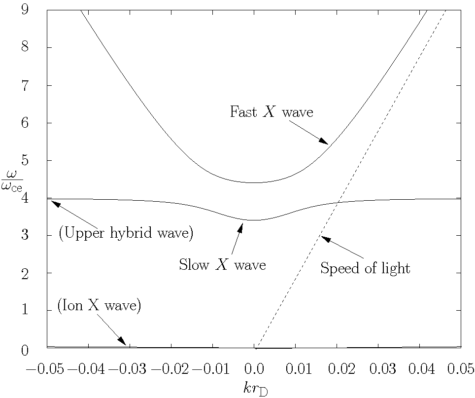
(a) Dispersion diagram

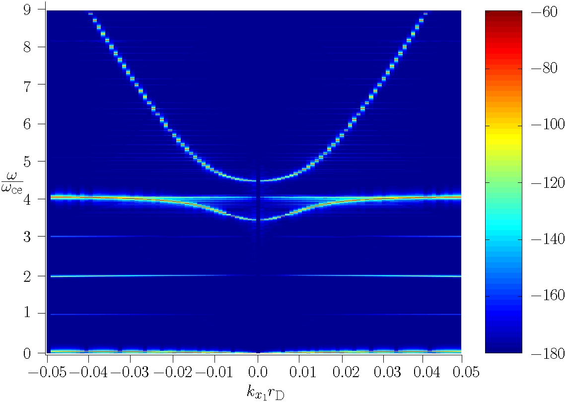
(b) Power spectrum

Figure 13: Dispersion diagram for the high frequency electromagnetic extraordinary mode, obtained from cold plasma fluid theory, and power spectrum (decibel) of the transverse part $E_{2}$ of the electric field obtained from Vlasov simulation; $\omega_{\mathrm{uh}}=4\omega_{\mathrm{ce}}$. After Eliasson (2003).

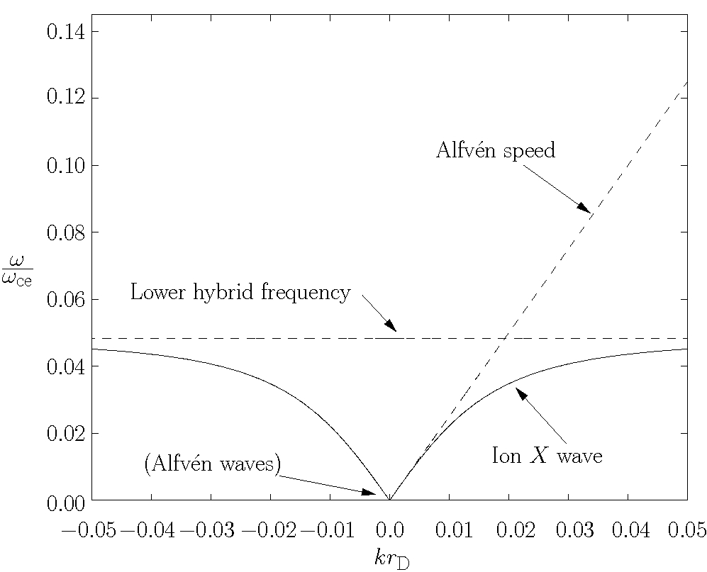
(a) Dispersion diagram

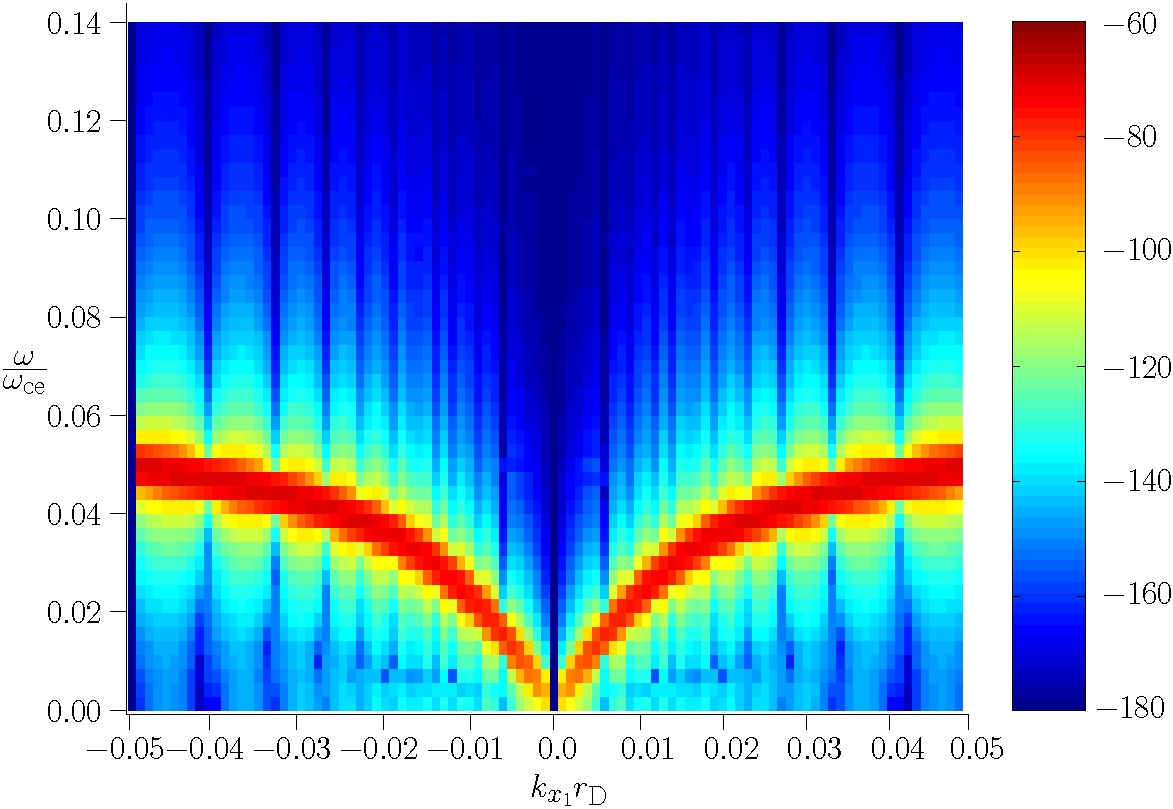
(b) Power spectrum

Figure 14: Dispersion diagram for the ion extraordinary wave, obtained from cold plasma fluid theory, and power spectrum (decibel) of the transverse part $E_{2}$ of the electric field obtained from the Vlasov simulation. The waves go over to Alfvén waves at small $k_{x1}$ and to lower hybrid hybrid oscillations at large $k_{x1}$; $\omega_{\mathrm{uh}}=4\omega_{\mathrm{ce}}$, $m_{\mathrm{i}}/m_{\mathrm{e}}=400$. After Eliasson (2003).

In Fig. 14, we compare theory with a closeup of the low-frequency part of the energy spectrum obtained in the Vlasov simulation. For the low frequency electromagnetic waves perpendicular to the magnetic field, An approximate dispersion relation obtained from a cold fluid description of ions and electrons is given by Goldston and Rutherford (1997) as

$$\frac{c^{2}k^{2}}{\omega^{2}}\bigg{(}\frac{\omega_{\mathrm{ci}}^{2}-\omega^{2}+\omega_{\mathrm{pi}}^{2}}{\omega_{\mathrm{ci}}^{2}-\omega^{2}}+\frac{\omega_{\mathrm{pe}}^{2}}{\omega_{\mathrm{ce}}^{2}}\bigg{)} =\bigg{(}\frac{\omega_{\mathrm{ci}}^{2}-\omega^{2}+\omega_{\mathrm{pi}}^{2}}{\omega_{\mathrm{ci}}^{2}-\omega^{2}}+\frac{\omega_{\mathrm{pe}}^{2}}{\omega_{\mathrm{ce}}^{2}}\bigg{)}^{2}-\bigg{(}\frac{\omega_{\mathrm{pi}}^{2}\omega}{\omega_{\mathrm{ci}}(\omega_{\mathrm{ci}}^{2}-\omega^{2})}\bigg{)}^{2}$$ (165)

with $c/v_{\mathrm{th,e}}=50$, $\omega_{\mathrm{uh}}/\omega_{\mathrm{ce}}=4$ and $\omega_{\mathrm{pe}}/\omega_{\mathrm{ce}}=\sqrt{15}$. For numerical efficiency we use the mass ratio $m_{\mathrm{i}}/m_{\mathrm{e}}=400$ between the ion and electron masses, which gives the ratios $\omega_{\mathrm{pi}}/\omega_{\mathrm{ce}}=\sqrt{15}/20$ and $\omega_{\mathrm{ci}}/\omega_{\mathrm{ce}}=1/400$. Eq. (165) is solved for $\omega/\omega_{\mathrm{ce}}$ and displayed in Fig. 14(a). For large $k_{x1}$, the dispersion curve approaches the lower hybrid frequency $\omega_{\mathrm{lh}}$, approximately given by

$$\omega_{\mathrm{lh}}^{-2}=\omega_{\mathrm{pi}}^{-2}+(\omega_{\mathrm{ci}}\omega_{\mathrm{ce}})^{-1}$$ (166)

and which is indicated in Fig. 14(a). For very small $k_{x1}\lambda_{e}<1$, we see in Fig. 14(a) that the dispersion curve approaches the one for Alfvén waves, governed by the dispersion relation

$$\omega^{2}=v_{A}^{2}k^{2},$$ (167)

where $v_{A}=c\omega_{ci}/\omega_{pi}$ is the Alfvén speed. The energy spectrum for the low frequency waves in Fig. 14(b) shows good similarity with the dispersion curve for the low frequency wave in Fig. 14(a). The width of the energy bands in the power spectrum is the frequency resolution obtained in the simulation; a longer simulation would resolve the waves more. The frequencies of the waves in Fig. 14(b) for large $k$ is slightly higher than the corresponding frequencies in the dispersion diagram in Fig. 14(a), which probably is a thermal effect, not included in the cold plasma fluid model.

In the Vlasov simulation presented here, the simulation domain was restricted to one spatial dimension with ${0\leq x_{1}\leq 2000\pi}$ and two velocity dimensions, plus time. The Fourier transformed velocity domain was ${0\leq\eta_{1}\leq 10}$ and ${-10\leq\eta_{2}\leq 10}$ for the electrons, and ${0\leq\eta_{1}\leq 200}$ and ${-200\leq\eta_{2}\leq 200}$ for the ions, with the number of intervals ${N_{x1}=100}$ in space and ${N_{\eta_{1}}=30}$ and ${2N_{\eta_{2}}=60}$ in the Fourier transformed velocity space. The initial conditions for the electrons and ions were set to $\widehat{f}_{\mathrm{e}}(x_{1},x_{2},\eta_{1},\eta_{2},0)=n(x)\widehat{f}_{\mathrm{e},0}(\eta_{1},\eta_{2})$ and $\widehat{f}_{\mathrm{i}}(x_{1},x_{2},\eta_{1},\eta_{2},0)=n(x)\widehat{f}_{\mathrm{i},0}(\eta_{1},\eta_{2})$, respectively, with the density perturbation

$$n(x)=1+10^{-7}\sum_{i_{1}=1}^{49}i_{1}\sin(0.05i_{1}x_{1})$$ (168)

so that all wavemodes were excited with low amplitudes, making the problem close to linear. The electron and ion distribution functions were set to

$$\widehat{f}_{\mathrm{e},0}(\eta_{1},\eta_{2}) =\frac{1}{(2\pi)^{2}}\exp\bigg{[}-\frac{1}{2}(\eta_{1}^{2}+\eta_{2}^{2})\bigg{]}$$ (169)

and

$$\widehat{f}_{\mathrm{i},0}(\eta_{1},\eta_{2}) =\frac{1}{(2\pi)^{2}}\exp\bigg{[}-\frac{1}{2}(\eta_{1}^{2}+\eta_{2}^{2})\bigg{(}\frac{v_{\mathrm{th,e}}}{v_{\mathrm{th,i}}}\bigg{)}^{-2}\bigg{]}$$ (170)

respectively. The number of time steps taken was $N_{t}=97\,280$; the end time was $t_{\mathrm{end}}=8340$. No numerical dissipation was used. The ion-electron mass ratio was $m_{\mathrm{i}}/m_{\mathrm{e}}=400$ and the ion and electron temperatures were set equal, $T_{\mathrm{i}}=T_{\mathrm{e}}$, giving the factor $(v_{\mathrm{th,e}}/v_{\mathrm{th,i}})^{-2}=1/400$ in Eq. (170).

VI The three-dimensional Vlasov equation

We here discuss the extension of the Fourier transform method to the Fourier transformed Vlasov equation in full three spatial and three velocity dimensions, including external and self-consistent magnetic fields. Again, in the design of well-posed absorbing boundary conditions in the Fourier transformed velocity space, special care has to be taken with the magnetic field, which enters into the formulation of the boundary condition.

The Fourier transformed Vlasov equation (13) can be cast into the normalized form

$$\frac{\partial\widehat{f}_{\mathrm{\alpha}}}{\partial t}-\mathrm{i}\boldsymbol{\nabla}_{\textbf{x}}\cdot\boldsymbol{\nabla}_{\boldsymbol{\eta}}\widehat{f}_{\mathrm{\alpha}}-\frac{Q_{\mathrm{\alpha}}}{M_{\mathrm{\alpha}}}\left\{\mathrm{i}{\bf E}\cdot\boldsymbol{\eta}\widehat{f}_{\mathrm{\alpha}}+\boldsymbol{\nabla}_{\boldsymbol{\eta}}\cdot\left[({\bf B}\times\boldsymbol{\eta})\widehat{f}_{\mathrm{\alpha}}\right]\right\}=0,$$ (171)

where $t$ is normalized by $\omega_{\mathrm{pe}}^{-1}$, v by $v_{\rm Te}$, x by $r_{\rm De}$, $\boldsymbol{\eta}$ by $v_{\rm Te}^{-1}$, $\widehat{f}_{\mathrm{\alpha}}$ by $n_{0}$, ${\bf E}$ by $v_{\rm Te}^{2}r_{\rm De}^{-1}(m_{\rm e}/e)$, and ${\bf B}$ by $\omega_{\rm pe}(m_{\rm e}/e)$. Here we defined $Q_{\alpha}=q_{\alpha}/e$ and $M_{\alpha}=m_{\alpha}/m_{\rm e}$, where we assume electrons and singly charged ions, so that $Q_{\rm i}=1$, $Q_{\rm e}=-1$, $M_{\rm i}=m_{\rm i}/m_{\rm e}$, and $M_{\rm e}=1$. The equations for the potentials, (31) and (32), take normalized form

$$\frac{\partial{\bf A}}{\partial t} ={\bf\Gamma}, \frac{\partial{\bf\Gamma}}{\partial t} =\frac{c^{2}}{v_{\rm Te}^{2}}\nabla_{\textbf{x}}^{2}{\bf A}+{\bf j},$$ (172)

$$-\nabla_{\textbf{x}}^{2}\Phi =\rho+\boldsymbol{\nabla}_{\textbf{x}}\cdot{\bf\Gamma},$$ (173)

and the electric and magnetic fields (33) and (34) are obtained as

$${\bf E}=-\boldsymbol{\nabla}_{\textbf{x}}\Phi-{\bf\Gamma},$$ (174)

$${\bf B}={\bf B}_{0}+\boldsymbol{\nabla}_{\textbf{x}}\times{\bf A},$$ (175)

where $\Phi$ is normalized by $v_{\rm Te}^{2}(m_{\rm e}/e)$, ${\bf A}$ by $v_{\rm Te}(m_{\rm e}/e)$, ${\bf\Gamma}$ by $\omega_{\rm pe}v_{\rm Te}(m_{\rm e}/e)$. $\rho$ by $en_{0}$, and ${\bf j}$ by $en_{0}v_{\rm Te}$. Using Eqs. (14) and (15) in Eqs. (7) and (8), the normalized charge and current densities are obtained as

$$\rho =(2\pi)^{3}[\Re(\widehat{f}_{\rm i})_{\boldsymbol{\eta}=\mathbf{0}}-\Re(\widehat{f}_{\rm e})_{\boldsymbol{\eta}=\mathbf{0}}],$$ (176)

and

$${\bf j} =(2\pi)^{3}[\boldsymbol{\nabla}_{\boldsymbol{\eta}}\Im(\widehat{f}_{\rm i})_{\boldsymbol{\eta}=\mathbf{0}}-\boldsymbol{\nabla}_{\boldsymbol{\eta}}\Im(\widehat{f}_{\rm e})_{\boldsymbol{\eta}=\mathbf{0}}],$$ (177)

respectively.

VI.1 Restriction to a bounded domain

In order to adapt the Fourier transformed Vlasov Maxwell system for numerical simulations, it must be restricted to a bounded domain. The computational domain is restricted to ${0\leq x_{1}<L_{1}}$, ${0\leq x_{2}<L_{2}}$, ${0\leq x_{3}<L_{3}}$, $0\leq\eta_{1}\leq\eta_{{\rm max},{1\mathrm{\alpha}}}$, $-\eta_{{\rm max},2\mathrm{\alpha}}\leq\eta_{2}\leq\eta_{{\rm max},2\mathrm{\alpha}}$, and $-\eta_{{\rm max},3\mathrm{\alpha}}\leq\eta_{3}\leq\eta_{{\rm max},3\mathrm{\alpha}}$. Here $\mathrm{\alpha}$ (equal to $e$ for electrons and $i$ for ions) is introduced so that different domain sizes can be used in $\boldsymbol{\eta}$ space for the ion and electron distribution functions. For negative $\eta_{1}$, the symmetry $\widehat{f}(x_{1},x_{2},x_{3},\eta_{1},\eta_{2},\eta_{3},t)=\widehat{f}^{*}(x_{1},x_{2},x_{3},-\eta_{1},-\eta_{2},-\eta_{3},t)$ is used to obtain function values; it is therefore not necessary to numerically represent the solution for negative $\eta_{1}$ if the solution is represented for negative $\eta_{2}$ and $\eta_{3}$.

VI.2 Outflow boundary conditions in Fourier transformed velocity space

In this section, we will derive well-posed boundary conditions for the Vlasov equation in $\boldsymbol{\eta}$ space. Writing out the terms of the Fourier transformed Vlasov equation (171), we have

$$\begin{split}&\frac{\partial\widehat{f}_{\mathrm{\alpha}}}{\partial t}-\mathrm{i}\frac{\partial^{2}\widehat{f}_{\mathrm{\alpha}}}{\partial x_{1}\partial\eta_{1}}-\mathrm{i}\frac{\partial^{2}\widehat{f}_{\mathrm{\alpha}}}{\partial x_{2}\partial\eta_{2}}-\mathrm{i}\frac{\partial^{2}\widehat{f}_{\mathrm{\alpha}}}{\partial x_{3}\partial\eta_{3}}-\frac{Q_{\mathrm{\alpha}}}{M_{\mathrm{\alpha}}}\bigg{[}\mathrm{i}(E_{1}\eta_{1}+E_{2}\eta_{2}+E_{3}\eta_{3})\widehat{f}_{\mathrm{\alpha}}\\ &+(B_{2}\eta_{3}-B_{3}\eta_{2})\frac{\partial\widehat{f}_{\mathrm{\alpha}}}{\partial\eta_{1}}+(B_{3}\eta_{1}-B_{1}\eta_{3})\frac{\partial\widehat{f}_{\mathrm{\alpha}}}{\partial\eta_{2}}+(B_{1}\eta_{2}-B_{2}\eta_{1})\frac{\partial\widehat{f}_{\mathrm{\alpha}}}{\partial\eta_{3}}\bigg{]}=0.\\ \end{split}$$ (178)

In position space, periodic boundary conditions

$$\widehat{f}_{\mathrm{\alpha}}(x_{1}+L_{1},x_{2},x_{3},\eta_{1},\eta_{2},\eta_{3},t) =\widehat{f}_{\mathrm{\alpha}}(x_{1},x_{2},x_{3},\eta_{1},\eta_{2},\eta_{3},t),$$ (179)

$$\widehat{f}_{\mathrm{\alpha}}(x_{1},x_{2}+L_{2},x_{3},\eta_{1},\eta_{2},\eta_{3},t) =\widehat{f}_{\mathrm{\alpha}}(x_{1},x_{2},x_{3},\eta_{1},\eta_{2},\eta_{3},t),$$ (180)

$$\widehat{f}_{\mathrm{\alpha}}(x_{1},x_{2},x_{3}+L_{3},\eta_{1},\eta_{2},\eta_{3},t) =\widehat{f}_{\mathrm{\alpha}}(x_{1},x_{2},x_{3},\eta_{1},\eta_{2},\eta_{3},t).$$ (181)

are used for both the distribution functions and the electromagnetic fields. The artificial boundaries at $\eta_{1}=\eta_{{\rm max},1\mathrm{\alpha}}$, $\eta_{2}=\pm\eta_{{\rm max},2\mathrm{\alpha}}$ and $\eta_{3}=\pm\eta_{{\rm max},3\mathrm{\alpha}}$ must be treated with care so that they do not give rise to reflections of waves or to instabilities. The strategy is to let outgoing waves pass over the boundaries, and to set incoming waves to zero. The problem of separating outgoing waves from incoming waves is solved by employing the spatial Fourier series expansions (transforms). In order to explore the idea, one can study the reduced initial value problem with a constant external magnetic field ${{\bf B}={\bf B}_{0}}$ and a zero electric field ${\bf E}={\bf 0}$,

$$\begin{split}&\frac{\partial\widehat{f}_{\mathrm{\alpha}}}{\partial t}-\mathrm{i}\frac{\partial^{2}\widehat{f}_{\mathrm{\alpha}}}{\partial x_{1}\partial\eta_{1}}-\mathrm{i}\frac{\partial^{2}\widehat{f}_{\mathrm{\alpha}}}{\partial x_{2}\partial\eta_{2}}-\mathrm{i}\frac{\partial^{2}\widehat{f}_{\mathrm{\alpha}}}{\partial x_{3}\partial\eta_{3}}-\frac{Q_{\mathrm{\alpha}}}{M_{\mathrm{\alpha}}}\bigg{[}(B_{2,0}\eta_{3}-B_{3,0}\eta_{2})\frac{\partial\widehat{f}_{\mathrm{\alpha}}}{\partial\eta_{1}}\\ &+(B_{3,0}\eta_{1}-B_{1,0}\eta_{3})\frac{\partial\widehat{f}_{\mathrm{\alpha}}}{\partial\eta_{2}}+(B_{1,0}\eta_{2}-B_{2,0}\eta_{1})\frac{\partial\widehat{f}_{\mathrm{\alpha}}}{\partial\eta_{3}}\bigg{]}=0,\\ \end{split}$$ (182)

$$\widehat{f}_{\mathrm{\alpha}}(x_{1},x_{2},x_{3},\eta_{1},\eta_{2},\eta_{3},t)_{t=0}=\widehat{f}_{\mathrm{\alpha}0}(x_{1},x_{2},x_{3},\eta_{1},\eta_{2},\eta_{3}).$$ (183)

By introducing the spatial Fourier series pairs in ($x_{1}$, $x_{2}$, $x_{3}$) space,

$$\widetilde{\phi}_{1,i_{1}} ={\rm F}_{1}\phi_{1}=\frac{1}{L_{1}}\int_{0}^{L_{1}}\phi_{1}(x_{1})e^{-\mathrm{i}k_{x_{1}}x_{1}}\mathrm{d}x_{1}$$ (184)

$$\phi_{1} ={\rm F}_{1}^{-1}\widetilde{\phi}_{1}=\sum_{i_{1}=-\infty}^{\infty}\widetilde{\phi}_{1,i_{1}}e^{\mathrm{i}k_{x_{1}}x_{1}}$$ (185)

$$k_{x_{1}} =\frac{2\pi i_{1}}{L_{1}},\quad i_{1}=0,\,\pm 1,\,\pm 2,\,\ldots,$$ (186)

$$\widetilde{\phi}_{2,i_{2}} ={\rm F}_{2}\phi_{2}=\frac{1}{L_{2}}\int_{0}^{L_{2}}\phi_{2}(x_{2})e^{-\mathrm{i}k_{x_{2}}x_{2}}\mathrm{d}x_{2}$$ (187)

$$\phi_{2} ={\rm F}_{2}^{-1}\widetilde{\phi}_{2}=\sum_{i_{2}=-\infty}^{\infty}\widetilde{\phi}_{2,i_{2}}e^{\mathrm{i}k_{x_{2}}x_{2}}$$ (188)

$$k_{x_{2}} =\frac{2\pi i_{2}}{L_{2}},\quad i_{2}=0,\,\pm 1,\,\pm 2,\,\ldots$$ (189)

and

$$\widetilde{\phi}_{3,i_{3}} ={\rm F}_{3}\phi_{3}=\frac{1}{L_{3}}\int_{0}^{L_{3}}\phi_{3}(x_{3})e^{-\mathrm{i}k_{x_{3}}x_{3}}\mathrm{d}x_{3},$$ (190)

$$\phi_{3} ={\rm F}_{3}^{-1}\widetilde{\phi}_{3}=\sum_{i_{3}=-\infty}^{\infty}\widetilde{\phi}_{3,i_{3}}e^{\mathrm{i}k_{x_{3}}x_{3}},$$ (191)

$$k_{x_{3}} =\frac{2\pi i_{3}}{L_{3}},\quad i_{3}=0,\,\pm 1,\,\pm 2,\,\ldots$$ (192)

respectively, and Fourier-transforming Eq. (182) in all spatial directions, one obtains a new differential equation for the unknown function $\widetilde{f}(k_{x_{1}},k_{x_{2}},k_{x_{3}},\eta_{1},\eta_{2},\eta_{3},t)$,

$$\begin{split}\frac{\partial\widetilde{f_{\mathrm{\alpha}}}}{\partial t}&+\bigg{[}k_{x_{1}}-\frac{Q_{\mathrm{\alpha}}}{M_{\mathrm{\alpha}}}(B_{2,0}\eta_{3}-B_{3,0}\eta_{2})\bigg{]}\frac{\partial\widetilde{f}_{\mathrm{\alpha}}}{\partial\eta_{1}}\\ &+\bigg{[}k_{x_{2}}-\frac{Q_{\mathrm{\alpha}}}{M_{\mathrm{\alpha}}}(B_{3,0}\eta_{1}-B_{1,0}\eta_{3})\bigg{]}\frac{\partial\widetilde{f}_{\mathrm{\alpha}}}{\partial\eta_{2}}\\ &+\bigg{[}k_{x_{3}}-\frac{Q_{\mathrm{\alpha}}}{M_{\mathrm{\alpha}}}(B_{1,0}\eta_{2}-B_{2,0}\eta_{1})\bigg{]}\frac{\partial\widetilde{f}_{\mathrm{\alpha}}}{\partial\eta_{3}}=0,\end{split}$$ (193)

with the initial condition

$$\widetilde{f}_{\mathrm{\alpha}}(k_{x_{1}},k_{x_{2}},k_{x_{3}},\eta_{1},\eta_{2},\eta_{3},t)_{t=0}=\widetilde{f}_{\mathrm{\alpha}0}(k_{x_{1}},k_{x_{2}},k_{x_{3}},\eta_{1},\eta_{2},\eta_{3}).$$ (194)

Equation (193) is a hyperbolic equation for which the initial values are transported along the characteristic curves, given by

$$\frac{\mathrm{d}\eta_{1}(t)}{\mathrm{d}t} =k_{x_{1}}-\frac{Q_{\mathrm{\alpha}}}{M_{\mathrm{\alpha}}}(B_{2,0}\eta_{3}-B_{3,0}\eta_{2}),$$ (195)

$$\frac{\mathrm{d}\eta_{2}(t)}{\mathrm{d}t} =k_{x_{2}}-\frac{Q_{\mathrm{\alpha}}}{M_{\mathrm{\alpha}}}(B_{3,0}\eta_{1}-B_{1,0}\eta_{3}),$$ (196)

$$\frac{\mathrm{d}\eta_{3}(t)}{\mathrm{d}t} =k_{x_{3}}-\frac{Q_{\mathrm{\alpha}}}{M_{\mathrm{\alpha}}}(B_{1,0}\eta_{2}-B_{2,0}\eta_{1}).$$ (197)

Along the boundary $\eta_{1}=\eta_{{\rm max},\mathrm{\alpha}1}$, Eq. (195) describes an outflow of data when $k_{x_{1}}-({Q_{\mathrm{\alpha}}}/{M_{\mathrm{\alpha}}})(B_{2,0}\eta_{3}-B_{3,0}\eta_{2})>0$ and an inflow of data when $k_{x_{1}}-({Q_{\mathrm{\alpha}}}/{M_{\mathrm{\alpha}}})(B_{2,0}\eta_{3}-B_{3,0}\eta_{2})<0$. A well-posed boundary condition is to set the inflow to zero at the boundary, i.e.,

$$(\widetilde{f}_{\mathrm{\alpha}})_{\eta_{1}=\eta_{{\rm max},\mathrm{\alpha}1}}=0,\hskip 14.22636ptk_{x_{1}}-\frac{Q_{\mathrm{\alpha}}}{M_{\mathrm{\alpha}}}(B_{2,0}\eta_{3}-B_{3,0}\eta_{2})<0,$$ (198)

which can be expressed with the help of the Heaviside step function $H$ as

$$\widetilde{f}_{\mathrm{\alpha}}=H\bigg{[}k_{x_{1}}-\frac{Q_{\mathrm{\alpha}}}{M_{\mathrm{\alpha}}}(B_{2,0}\eta_{3}-B_{3,0}\eta_{2})\bigg{]}\widetilde{f}_{\mathrm{\alpha}},\hskip 14.22636pt\eta_{1}=\eta_{{\rm max},\mathrm{\alpha}1},$$ (199)

where

$$H(\xi)=\left\{\begin{array}[]{l}1,\hskip 14.22636pt\xi\geq 0\\ 0,\hskip 14.22636pt\xi<0,\end{array}\right.$$ (200)

The boundary condition (199) allows outgoing waves to pass over the boundary and to be removed, while incoming waves are set to zero; the removal of the outgoing waves corresponds to the losing of information about the finest structures in velocity space. Inverse Fourier transforming Eq. (199) then gives the boundary condition for the original problem (182) as

$$\widehat{f}_{\mathrm{\alpha}}={\rm F}_{1}^{-1}H\bigg{[}k_{x_{1}}-\frac{Q_{\mathrm{\alpha}}}{M_{\mathrm{\alpha}}}(B_{2,0}\eta_{3}-B_{3,0}\eta_{2})\bigg{]}{\rm F}_{1}\widehat{f}_{\mathrm{\alpha}},\hskip 14.22636pt\eta_{1}=\eta_{{\rm max},\mathrm{\alpha}1}.$$ (201)

The operator ${\rm F}_{1}^{-1}H[k_{x_{1}}-({Q_{\mathrm{\alpha}}}/{M_{\mathrm{\alpha}}})(B_{2,0}\eta_{3}-B_{3,0}\eta_{2})]{\rm F}_{1}$ is a projection operator which removes incoming waves at the boundary $\eta_{1}=\eta_{{\rm max},\mathrm{\alpha}1}$. Similarly, the boundary conditions at $\eta_{2}=\pm\eta_{{\rm max},\mathrm{\alpha}2}$ and $\eta_{3}=\pm\eta_{{\rm max},\mathrm{\alpha}3}$ become

$$\widehat{f}_{\mathrm{\alpha}} ={\rm F}_{2}^{-1}H\bigg{[}k_{x_{2}}-\frac{Q_{\mathrm{\alpha}}}{M_{\mathrm{\alpha}}}(B_{3,0}\eta_{1}-B_{1,0}\eta_{3})\bigg{]}{\rm F}_{2}\widehat{f}_{\mathrm{\alpha}},\hskip 14.22636pt\eta_{2}=\eta_{{\rm max},\mathrm{\alpha}2},$$ (202)

$$\widehat{f}_{\mathrm{\alpha}} ={\rm F}_{2}^{-1}H\bigg{[}-k_{x_{2}}+\frac{Q_{\mathrm{\alpha}}}{M_{\mathrm{\alpha}}}(B_{3,0}\eta_{1}-B_{1,0}\eta_{3})\bigg{]}{\rm F}_{2}\widehat{f}_{\mathrm{\alpha}},\hskip 14.22636pt\eta_{2}=-\eta_{{\rm max},\mathrm{\alpha}2},$$ (203)

and

$$\widehat{f}_{\mathrm{\alpha}} ={\rm F}_{3}^{-1}H\bigg{[}k_{x_{3}}-\frac{Q_{\mathrm{\alpha}}}{M_{\mathrm{\alpha}}}(B_{1,0}\eta_{2}-B_{2,0}\eta_{1})\bigg{]}{\rm F}_{3}\widehat{f}_{\mathrm{\alpha}},\hskip 14.22636pt\eta_{3}=\eta_{{\rm max},\mathrm{\alpha}3},$$ (204)

$$\widehat{f}_{\mathrm{\alpha}} ={\rm F}_{3}^{-1}H\bigg{[}-k_{x_{3}}+\frac{Q_{\mathrm{\alpha}}}{M_{\mathrm{\alpha}}}(B_{1,0}\eta_{2}-B_{2,0}\eta_{1})\bigg{]}{\rm F}_{3}\widehat{f}_{\mathrm{\alpha}},\hskip 14.22636pt\eta_{3}=-\eta_{{\rm max},\mathrm{\alpha}3},$$ (205)

respectively.

In order to find well-posed boundary conditions in $\boldsymbol{\eta}$ space in the case when ${\bf B}$ varies both in space and time, Eq. (178) is rewritten in the form

$$\begin{split}\frac{\partial\widehat{f}_{\mathrm{\alpha}}}{\partial t}+&\theta_{\mathrm{\alpha}1}\frac{\partial}{\partial\eta_{1}}\bigg{[}-\mathrm{i}\frac{\partial}{\partial x_{1}}-\beta_{01}\bigg{]}(\widehat{f}_{\mathrm{\alpha}}\theta_{\mathrm{\alpha}1}^{-1})\\ +&\theta_{\mathrm{\alpha}2}\frac{\partial}{\partial\eta_{2}}\bigg{[}-\mathrm{i}\frac{\partial}{\partial x_{2}}-\beta_{02}\bigg{]}(\widehat{f}_{\mathrm{\alpha}}\theta_{\mathrm{\alpha}2}^{-1})\\ +&\theta_{\mathrm{\alpha}3}\frac{\partial}{\partial\eta_{3}}\bigg{[}-\mathrm{i}\frac{\partial}{\partial x_{3}}-\beta_{03}\bigg{]}(\widehat{f}_{\mathrm{\alpha}}\theta_{\mathrm{\alpha}3}^{-1})+\mathrm{i}(E_{1}\eta_{1}+E_{2}\eta_{2}+E_{3}\eta_{3})\widehat{f}_{\mathrm{\alpha}}=0,\end{split}$$ (206)

where the phase factors $\theta_{\mathrm{\alpha}1}$, $\theta_{\mathrm{\alpha}2}$ and $\theta_{\mathrm{\alpha}3}$ are

$$\theta_{\mathrm{\alpha}1} =\exp\left[\mathrm{i}\int_{0}^{x_{1}}(\beta_{1}-\beta_{01})\,\mathrm{d}x_{1}\right],$$ (207)

$$\theta_{\mathrm{\alpha}2} =\exp\left[\mathrm{i}\int_{0}^{x_{2}}(\beta_{2}-\beta_{02})\,\mathrm{d}x_{2}\right],$$ (208)

and

$$\theta_{\mathrm{\alpha}3} =\exp\left[\mathrm{i}\int_{0}^{x_{3}}(\beta_{3}-\beta_{03})\,\mathrm{d}x_{3}\right],$$ (209)

respectively, and where

$$\beta_{1}=\frac{Q_{\alpha}}{M_{\alpha}}(B_{2}\eta_{3}-B_{3}\eta_{2}),\qquad\beta_{01}=\frac{1}{L_{1}}\int_{0}^{L_{1}}\beta_{1}\,\mathrm{d}x_{1},$$ (210)

$$\beta_{2}=\frac{Q_{\alpha}}{M_{\alpha}}(B_{3}\eta_{1}-B_{1}\eta_{3}),\qquad\beta_{02}=\frac{1}{L_{2}}\int_{0}^{L_{2}}\beta_{2}\,\mathrm{d}x_{2},$$ (211)

and

$$\beta_{3}=\frac{Q_{\alpha}}{M_{\alpha}}(B_{1}\eta_{2}-B_{2}\eta_{1}),\qquad\beta_{03}=\frac{1}{L_{3}}\int_{0}^{L_{3}}\beta_{3}\,\mathrm{d}x_{3}.$$ (212)

The form (206) of the Vlasov equation makes it possible to introduce stable numerical boundary conditions in $\boldsymbol{\eta}$ space in a systematic manner. Furthermore, $\int_{0}^{x_{1}}(\beta_{1}-\beta_{01})\mathrm{d}x_{1}$, $\int_{0}^{x_{2}}(\beta_{2}-\beta_{02})\mathrm{d}x_{2}$ and $\int_{0}^{x_{3}}(\beta_{3}-\beta_{03})\mathrm{d}x_{3}$ are continuous and periodic in x space if ${\bf B}$ is continuous and periodic in x; this is the reason for the subtraction of the mean values $\beta_{01}$, $\beta_{02}$ and $\beta_{03}$ in the integrals.

By studying the flow of data in the $\eta_{1}$, $\eta_{2}$ and $\eta_{3}$ directions for $\widehat{f}_{\mathrm{\alpha}}\theta_{\mathrm{\alpha}1}^{-1}$, $\widehat{f}_{\mathrm{\alpha}}\theta_{\mathrm{\alpha}2}^{-1}$ and $\widehat{f}_{\mathrm{\alpha}}\theta_{\mathrm{\alpha}3}^{-1}$, respectively, one finds the outflow boundary conditions to be

$$\widehat{f}_{\mathrm{\alpha}} =\theta_{\mathrm{\alpha}1}{\rm F}_{1}^{-1}H(k_{x_{1}}-\beta_{01}){\rm F}_{1}(\widehat{f}_{\mathrm{\alpha}}\theta_{\mathrm{\alpha}1}^{-1}),\hskip 14.22636pt\eta_{1}=\eta_{{\rm max},\mathrm{\alpha}1},$$ (213)

$$\widehat{f}_{\mathrm{\alpha}} =\theta_{\mathrm{\alpha}2}{\rm F}_{2}^{-1}H(k_{x_{2}}-\beta_{02}){\rm F}_{2}(\widehat{f}_{\mathrm{\alpha}}\theta_{\mathrm{\alpha}2}^{-1}),\hskip 14.22636pt\eta_{2}=\eta_{{\rm max},\mathrm{\alpha}2},$$ (214)

$$\widehat{f}_{\mathrm{\alpha}} =\theta_{\mathrm{\alpha}2}{\rm F}_{2}^{-1}H(-k_{x_{2}}+\beta_{02}){\rm F}_{2}(\widehat{f}_{\mathrm{\alpha}}\theta_{\mathrm{\alpha}2}^{-1}),\hskip 14.22636pt\eta_{2}=-\eta_{{\rm max},\mathrm{\alpha}2},$$ (215)

$$\widehat{f}_{\mathrm{\alpha}} =\theta_{\mathrm{\alpha}3}{\rm F}_{3}^{-1}H(k_{x_{3}}-\beta_{03}){\rm F}_{3}(\widehat{f}_{\mathrm{\alpha}}\theta_{\mathrm{\alpha}3}^{-1}),\hskip 14.22636pt\eta_{2}=\eta_{{\rm max},\mathrm{\alpha}2},$$ (216)

$$\widehat{f}_{\mathrm{\alpha}} =\theta_{\mathrm{\alpha}3}{\rm F}_{3}^{-1}H(-k_{x_{3}}+\beta_{03}){\rm F}_{3}(\widehat{f}_{\mathrm{\alpha}}\theta_{\mathrm{\alpha}3}^{-1}),\hskip 14.22636pt\eta_{2}=-\eta_{{\rm max},\mathrm{\alpha}2}.$$ (217)

In the case when ${\bf B}$ is independent of x and $t$, the boundary conditions (213)–(214) reduce to the conditions (201)–(205). For the case where the domain is extended to negative $\eta_{1}$, we also have the boundary condition

$$\widehat{f}_{\mathrm{\alpha}}=\theta_{\mathrm{\alpha}1}{\rm F}_{1}^{-1}H(-k_{x_{1}}+\beta_{01}){\rm F}_{1}(\widehat{f}_{\mathrm{\alpha}}\theta_{\mathrm{\alpha}1}^{-1}),\hskip 14.22636pt\eta_{1}=-\eta_{{\rm max},\mathrm{\alpha}1},$$ (218)

which was used at a stage in the numerical algorithm. The well-posedness of these boundary conditions were proven by using that a positively definite energy integral was non-increasing (Eliasson, 2007).

VI.3 Electromagnetic electron waves

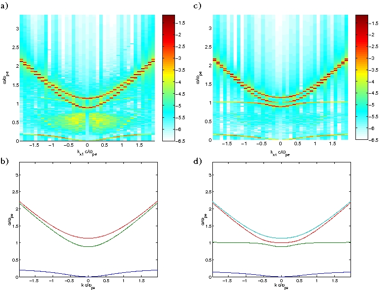
Figure 15: a) Amplitude spectrum (10-log scale) of $E_{2}$ for waves propagating parallel to the external magnetic field ($\theta=0$). b) Dispersion relations for the high-frequency R and L waves and the low-frequency whistler wave, propagating along the external magnetic field ($\theta=0$). c) Amplitude spectrum of $E_{2}$ for waves propagating with an angle $\theta=\pi/4$ to the external magnetic field, and d) dispersion relations for electron waves propagating with an angle of $\theta=\pi/4$ to the external magnetic field. Here $\omega_{\rm ce}/\omega_{\rm pe}=1/4$. After Eliasson (2007).

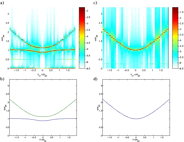
Figure 16: a) Amplitude spectrum (10-log scale) of $E_{3}$ for waves propagating perpendicularly to the external magnetic field ($\theta=\pi/2$), with the electric field perpendicular to the external magnetic field, and b) dispersion relations for the high-frequency slow and fast extraordinary (X-) modes, propagating perpendicularly to the external magnetic field ($\theta=\pi/2$). c) Amplitude spectrum of $E_{2}$ for waves propagating perpendicularly to the external magnetic field ($\theta=\pi/2$), with the electric field parallel to the magnetic field, and d) dispersion relations for the ordinary (O-) mode propagating perpendicularly ($\theta=\pi/2$) to the magnetic field. Here $\omega_{\rm ce}/\omega_{\rm pe}=1/4$. After Eliasson (2007).

The general dispersion relation for electron waves in a cold collisionless plasma with an external magnetic field is given by the Appleton-Hartree dispersion relation (Stix, 1992)

$$\frac{c^{2}k^{2}}{\omega^{2}} =1-\frac{2\omega_{\rm pe}^{2}(\omega^{2}-\omega_{\rm pe}^{2})/\omega^{2}}{2(\omega^{2}-\omega_{\rm pe}^{2})-\omega_{\rm ce}^{2}\sin^{2}\theta\pm\omega_{\rm ce}\Delta},$$ (219)

where $\Delta=[\omega_{\rm ce}^{2}\sin^{4}\theta+4\omega^{-2}(\omega^{2}-\omega_{\rm pe}^{2})^{2}\cos^{2}\theta]^{1/2}$ and $\theta$ is the angle between the external magnetic field and the wave vector. In order to assess that the Vlasov code reproduces these well-known wave modes in the plasma, we have simulated electromagnetic waves propagating at different angles to the magnetic field; see Figs. 15 and 16. In the simulations, we restricted the problem to one spatial dimension, along the $x_{1}$ axis, and used three velocity dimensions. The initial condition for the electron distribution function was a Maxwellian distribution (in normalized units)

$$\widehat{f}_{\rm e}=(2\pi)^{-3}\exp\left[-\frac{(\eta_{1}^{2}+\eta_{2}^{2}+\eta_{3}^{2})}{2}\right]$$ (220)

while for the ions we used

$$\widehat{f}_{\rm i}=(2\pi)^{-3}\exp\left[-\frac{(\eta_{1}^{2}+\eta_{2}^{2}+\eta_{3}^{2})}{2}\left(\frac{T_{\rm i}m_{\rm e}}{T_{\rm e}m_{\rm i}}\right)^{1/2}\right],$$ (221)

with $T_{\rm i}/T_{\rm e}=100$ and $m_{\rm i}/m_{\rm e}=1836$, and we chose $c/v_{\rm Te}=50$ for the electromagnetic waves. The magnetic field strength was chosen such that $\omega_{\rm ce}/\omega_{\rm pe}=1/4$, i.e. in our scaled unit we have $|{\bf B}_{0}|=1/4$. A low-amplitude noise (random numbers) were added to the vector potential ${\bf A}$ and to ${\bf\Gamma}$ so that all wave modes in the system were excited. The numerical parameters were chosen as $N_{x_{1}}=40$, $N_{x_{2}}=N_{x_{3}}=1$, $L_{1}=\pi\times 10^{3}$ (corresponding to $20\pi\,c/\omega_{\rm pe}$ in dimensional units), $N_{\eta_{1}}=N_{\eta_{2}}=N_{\eta_{3}}=20$, $\eta_{{\rm max},{\rm e}1}=\eta_{{\rm max},{\rm e}2}=\eta_{{\rm max},{\rm e}3}=6$, and $\eta_{{\rm max},{\rm i}1}=\eta_{{\rm max},{\rm i}2}=\eta_{{\rm max},{\rm i}3}=200$. The simulations were run with $8000$ time-steps with the fixed time interval $\Delta t=0.14$. In Figs. 15 and 16, we have Fourier transformed the electric field in space and time (with a Gaussian time window) to obtain the spatio-temporal wave spectrum. In panel a) of Fig. 15, we show the power spectrum for the transversal electric field component $E_{2}$, for waves propagating along the magnetic field lines. It is clearly seen that the wave energy is concentrated along the dispersion curves of the electromagnetic right-hand (R) and left-hand (L) circularly polarized waves, shown in in panel b). They are given by the dispersion relation

$$\frac{c^{2}k^{2}}{\omega^{2}} =1-\frac{\omega_{\rm pe}^{2}/\omega^{2}}{1-\omega_{\rm ce}/\omega}$$ (222)

and

$$\frac{c^{2}k^{2}}{\omega^{2}} =1-\frac{\omega_{\rm pe}^{2}/\omega^{2}}{1+\omega_{\rm ce}/\omega}$$ (223)

respectively, obtained by setting $\theta=0$ in Eq. (219). The R-wave is divided into a high-frequency branch (having the highest frequency) and the low-frequency electron whistler branch. We next made a simulation of waves propagating obliquely to the external magnetic field, which was chosen as $(B_{01},\,B_{02},\,B_{03})=(0.25,\,0.25,\,0)/\sqrt{2}$. The resulting amplitude spectrum of $E_{2}$ is presented in panel c) of Fig. 15, while the solutions of the dispersion relation (219) is plotted in panel d). Here, we can see the emergence of the slow $X$-mode which has a resonance somewhat higher than the plasma frequency $\omega=\omega_{\rm pe}$. Comparing panel c) and d), we see that the wave energy is concentrated at the dispersion curves. In Fig. (16), we are considering waves propagating perpendicularly to the magnetic field. Here, the external magnetic field is given by $(B_{01},\,B_{02},\,B_{03})=(0,\,0.25,\,0)$, and the energy spectrum in panel a) and c) are for the perpendicular (to the magnetic field direction) and parallel electric field components $E_{3}$ and $E_{2}$, respectively. The wave energy is concentrated at the dispersion curves for the cold plasma fast and slow X-modes displayed in panel b) and the O-mode plotted in panel d). The cold plasma dispersion relation for the ordinary (O-) mode and extraordinary (X-) mode, perpendicular to the magnetic field, is given by

$$\frac{c^{2}k^{2}}{\omega^{2}} =1-\frac{\omega_{\rm pe}^{2}}{\omega^{2}}$$ (224)

and

$$\frac{c^{2}k^{2}}{\omega^{2}} =1-\frac{\omega_{\rm pe}^{2}}{\omega^{2}}\frac{(\omega^{2}-\omega_{\rm pe}^{2})}{(\omega^{2}-\omega_{\rm pe}^{2}-\omega_{\rm ce}^{2})},$$ (225)

respectively, obtained by setting $\theta=\pi/2$ in Eq. (219). Also seen in panel a) at $\omega/\omega_{\rm pe}=0.5$ is an excitation of an electron Bernstein mode which starts at $\omega=2\omega_{ce}$ at small wavenumbers and has a resonance at $\omega=\omega_{\rm ce}$ for large wavenumbers.

VI.4 Temperature anisotropy driven whistler instability

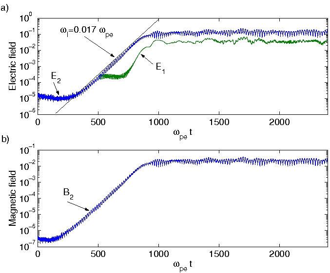
Figure 17: a) The maximum amplitude of the parallel and perpendicular electric field components $E_{1}$ and $E_{2}$, respectively, and b) the perpendicular magnetic field component $B_{2}$ (The parallel electric field $E_{1}$ is shown only for times $t>500\,\omega_{\rm pe}^{-1}$). After Eliasson (2007).

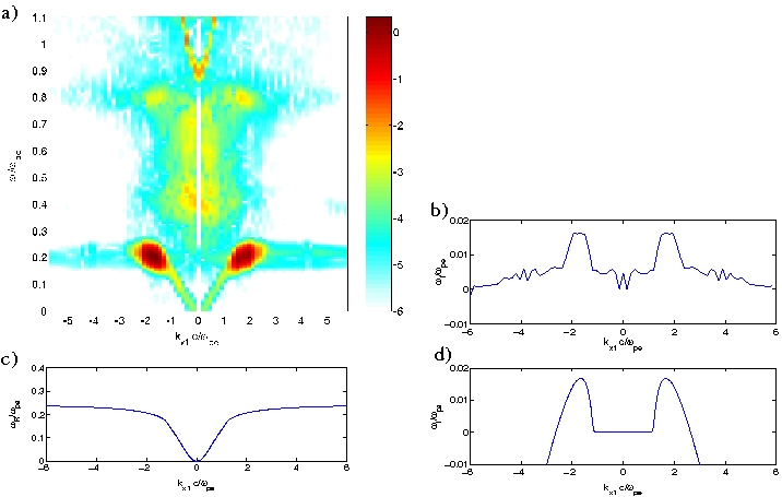
Figure 18: a) The spatio-temporal amplitude spectrum of the electric field component $E_{2}$, and b) the spatial amplitude spectrum at time $t=700\,\omega_{\rm pe}$. c) The real and d) imaginary parts of the frequency for whistler waves, obtained from the dispersion relation (228), in an anisotropic plasma with $T_{\perp}/T_{\parallel}=8$, $c/v_{{\rm Te}\parallel}=50$ and $\omega_{\rm ce}/\omega_{\rm pe}=0.25$. After Eliasson (2007).

In magnetized plasmas, there are often different temperatures parallel and perpendicular to the magnetic field direction. In this case, we may have a firehose instability if $T_{{\rm e}\parallel}>T_{{\rm e}\perp}$, or a whistler instability if $T_{{\rm e}\perp}>T_{{\rm e}\parallel}$. The latter case can have relevance both for the sun and for the Earth’s magnetosheath (Zhao et al., 1996; Gosling et al., 1989). In order to study the growth and saturation of the whistler instability, we carried out a simulation where the initial condition for the electrons was taken to be a bi-Maxwellian distribution function, where we used the temperature ratio $T_{{\rm e}\perp}/T_{{\rm e}\parallel}=8$. In the Fourier transformed velocity variables used in the simulation, the electron and ion distribution function takes the form

$$\widehat{f}_{\rm e}=(2\pi)^{-3}\exp\left[-\frac{(\eta_{1}^{2}+8\eta_{2}^{2}+8\eta_{3}^{2})}{2}\right],$$ (226)

while for the ions we used

$$\widehat{f}_{\rm i}=(2\pi)^{-3}\exp\left[-\frac{(\eta_{1}^{2}+\eta_{2}^{2}+\eta_{3}^{2})}{2}\left(\frac{T_{\rm i}m_{\rm e}}{T_{\rm e}m_{\rm i}}\right)^{1/2}\right],$$ (227)

with $T_{\rm i}/T_{{\rm e}\parallel}=100$ and $m_{\rm i}/m_{\rm e}=1836$. We use the same numerical parameters as in section VI.3, except that $\eta_{{\rm max},{\rm e}2}=\eta_{{\rm max},{\rm e}3}=3$ and we use a higher resolution in space such that $N_{x1}=80$. An adaptive time step was used in the simulation to maintain numerical stability (Eliasson, 2007). The numerical results are displayed in Figs. 17 and 18. The time-dependence of the maximum amplitude (over the spatial domain) of the perpendicular electric and magnetic field components $E_{2}$ and $B_{2}$ are shown in Fig. 17, and we see an exponential growth of the perpendicular electric field component $E_{2}$, with a growth rate of $\omega_{\rm I}\approx 0.017\omega_{\rm pe}$ [indicated by the solid line in panel a)] of both the electric and magnetic field. The initially almost purely electromagnetic waves saturate nonlinearly by exciting the electrostatic field component $E_{1}$ (see the upper panel of Fig. 17), and the amplitude of the perpendicular magnetic field fluctuations are at this point about 10 % of the external magnetic field. In order to compare the simulation result with theory, we have plotted the spatio-temporal amplitude spectrum of the perpendicular electric field component $E_{2}$ in panel a) of Fig. 18 (in a 10-log scale) where the Fourier transform in time was taken for waves between $\omega_{\rm pe}t=0$ and $\omega_{\rm pe}t=600$, with a Gaussian time window. In panel b), we have plotted the quantity $\omega_{\rm I}=(1/t_{1}){\rm ln}[|\widehat{E}_{2}(t_{1})|]+$constant where $\widehat{E}_{2}$ is the spatial Fourier transform of the electric field component $E_{2}$ at time $t=t_{1}$ and $t_{1}=700\,\omega_{pe}^{-1}$. Panel b) gives a rough estimate of the growth rate for different wavenumbers in the simulation. We see that there is a significant growth rate of waves with wavenumbers between $kc/\omega_{\rm pe}\approx 1.2$ and $kc/\omega_{\rm pe}\approx 2.6$. We have solved the dispersion relation for whistler waves in a plasma with a bi-Maxwellian electron distribution. In the one-dimensional case, and for immobile ions, it is (Stix, 1992)

$$\frac{k_{\parallel}^{2}c^{2}}{\omega_{\rm pe}^{2}}=\frac{T_{{\rm e}\perp}}{T_{{\rm e}\parallel}}-1+\frac{(\omega-\omega_{\rm ce})T_{{\rm e}\perp}/T_{{\rm e}\parallel}+\omega_{\rm ce}}{\sqrt{2}k_{\parallel}v_{{\rm Te}\parallel}}Z\left(\frac{\omega-\omega_{\rm ce}}{\sqrt{2}k_{\parallel}v_{{\rm Te}\parallel}}\right)$$ (228)

where $v_{{\rm Te}\parallel}=(k_{\rm B}T_{{\rm e}\parallel}/m_{\rm e})^{1/2}$ is the parallel electron thermal speed and

$$Z(\xi)=\mathrm{i}\sqrt{\pi}\exp(-\xi^{2})[1+{\rm erf}(\mathrm{i}\xi)]$$ (229)

is the plasma dispersion function. In the dispersion relation (228), we have neglected the electromagnetic displacement current term [corresponding to the first term in the right-hand side of Eq. (222)]. In panels c) and d) of Fig. 18, we have plotted the real and imaginary parts of the frequency, obtained from the dispersion relation (228), where we have used the simulation parameters $\omega_{\rm ce}/\omega_{\rm pe}=0.25$, $T_{{\rm e}\perp}/T_{{\rm e}\parallel}=8$ and $c/v_{{\rm Te}\parallel}=50$. Comparing panels a) and c), we see that for the undamped waves at small wavenumbers, the wave energy of the waves in the simulation is located along the dispersion curve of the whistler wave. Panels b) and d) show that the spectrum of the growing waves matches approximately the waves with positive growth rate obtained from the dispersion relation (228). We note that the maximum growth rate $\omega_{\rm I}\approx 0.017\,\omega_{\rm pe}$ in panel d) of Fig. 18 agrees well with the measured growth rate in panel a) of Fig. 17.

VII Extensions to incorporate relativistic and quantum effects

We here very briefly discuss the extensions of the Fourier technique for relativistic and quantum Vlasov equations.

VII.1 The relativistic Vlasov equation

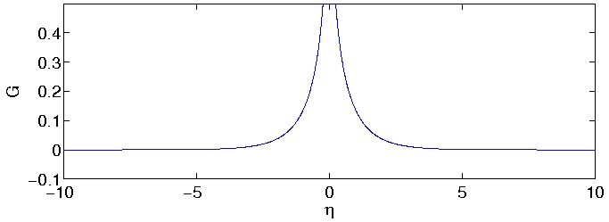
Figure 19: The function $G(\eta)$.

In the relativistic Vlasov equation, the relativistic gamma factor comes into play for particles moving close to the speed of light. This complicates the use of the Fourier transform technique to solve the Vlasov equation. As a model example we consider the one-dimensional Vlasov-Poisson system

$$\frac{\partial f}{\partial t}+\frac{p}{\gamma}\frac{\partial f}{\partial x}-E\frac{\partial f}{\partial p}=0,$$ (230)

$$\frac{\partial E}{\partial x}=1-\int_{-\infty}^{\infty}f\,dp$$ (231)

where the relativistic gamma factor is $\gamma=\sqrt{1+p^{2}}$, and $f$ describes the distribution of electrons in $(x,p)$ space where $p$ is the momentum. Here the distribution function $f$ has been normalized by $n_{0}/c$, time $t$ by $\omega_{pe}^{-1}$, space $x$ by $\lambda_{e}=c/\omega_{pe}$, momentum $p$ by $m_{e}c$, and the electric field $E$ by $m_{e}c^{2}/e\lambda_{e}$. Using the Fourier transform pair

$$f(x,p,t) =\int_{-\infty}^{\infty}\widehat{f}(x,\eta,t)e^{-i\eta p}\,d\eta,$$ (232)

$$\widehat{f}(x,\eta,t) =\frac{1}{2\pi}\int_{-\infty}^{\infty}f(x,v,t)e^{i\eta p}\,dp,$$ (233)

we have the Fourier transformed Vlasov-Poisson system

$$\frac{\partial\widehat{f}}{\partial t}-i\frac{\partial^{2}}{\partial x\partial\eta}(G*\widehat{f})+iE\eta\widehat{f}=0,$$ (234)

$$\frac{\partial E}{\partial x}=1-2\pi\widehat{f}(x,\eta,t)_{\eta=0},$$ (235)

where $*$ denotes convolution over $\eta$ space. Here

$$\begin{split}G&=\frac{1}{2\pi}\int_{-\infty}^{\infty}\gamma^{-1}e^{i\eta p}\,dp=\frac{1}{\pi}{\rm K}_{0}(|\eta|),\end{split}$$ (236)

where $K_{0}$ is the Bessel function of second kind of order $0$. The function $G(\eta)$, plotted in Fig. 19, grows like $[-\gamma_{E}-{\rm ln}(|\eta|/2)]/\pi$ for $|\eta|<1$, where $\gamma_{E}\approx 0.5772156649$ is the Euler-Mascheroni constant, and falls off like $\exp(-|\eta|)(2\pi|\eta|)^{-1/2}$ for $|\eta|>1$, and has the property that $\int_{-\infty}^{\infty}G\,d\eta=1$. The relativistic corrections are contained in $G$. For a weakly relativistic plasma, the distribution function $\widehat{f}$ is much wider and smoother in $\eta$ space than $G$, and hence we have $G*\widehat{f}\approx\widehat{f}$, i.e., $G$ then has the property of Dirac’s delta function and we retain the non-relativistic Fourier transformed Vlasov equation treated by Eliasson (2001). The numerical implementation of the convolution by $G$ and the well-posed absorbing boundary conditions in $\eta$ space are unsolved problems, and so are the extensions to higher dimensions. Since the function $G$ in Fig. 19 falls of exponentially for large $\eta$, the convolution integral in (234) can possibly be approximated by a truncated operator with compact support, and the problem with absorbing boundary conditions could potentially be solved using normal mode analysis similar to that of Engquist and Majda (1977, 1979).

VII.2 The Quantum Vlasov/Wigner equation

The quantum analogue to the Vlasov-Poisson system is the Wigner-Poisson model (Wigner, 1932; Roos, 1960; Tatarskii, 1983; Markowich et al., 1990). In three dimensions, the Wigner equation for electrons can be written

$$\frac{\partial f}{\partial t}+{\bf v}\cdot\nabla f=-\frac{iem_{e}^{3}}{(2\pi)^{3}\hbar^{4}}\int\!\!\!\int d^{3}\lambda\,d^{3}v^{\prime}e^{im_{e}({\bf v}-{\bf v}^{\prime})\cdot{\boldsymbol{\lambda}}/\hbar}\bigg{[}\phi\bigg{(}{\bf x}+\frac{\boldsymbol{\lambda}}{2},t\bigg{)}-\phi\bigg{(}{\bf x}-\frac{\boldsymbol{\lambda}}{2},t\bigg{)}\bigg{]}f({\bf x},{\bf v}^{\prime},t),$$ (237)

which is coupled with the Poisson equation with immobile ions

$$\nabla^{2}\phi=\frac{e}{\varepsilon_{0}}\left(\int fd^{3}v-n_{0}\right).$$ (238)

One can show that the Wigner equation converges to the Vlasov equation in the formal limit $\hbar\rightarrow 0$,

$$\frac{\partial f}{\partial t}+{\bf v}\cdot\nabla f=-\frac{e}{m_{e}}\nabla\phi\cdot\frac{\partial f}{\partial{\bf v}}.$$ (239)

It turns out that the Fourier technique in velocity space is well suited to solve the Wigner equation. As an example we will study the 1D Wigner-Poisson system (Manfredi, 2002)

$$\frac{\partial f}{\partial t}+v\frac{\partial f}{\partial x}=-\frac{iem_{e}}{(2\pi)\hbar^{2}}\int\!\!\!\int e^{im_{e}(v-v^{\prime}){\lambda}/\hbar}\bigg{[}\phi\bigg{(}{x}+\frac{\lambda}{2},t\bigg{)}-\phi\bigg{(}{x}-\frac{\lambda}{2},t\bigg{)}\bigg{]}f({x},{v}^{\prime},t)d\lambda\,dv^{\prime}$$ (240)

$$\frac{\partial^{2}\phi}{\partial x^{2}}=\frac{e}{\varepsilon_{0}}\left(\int fdv-n_{0}\right).$$ (241)

As it stands, the Wigner is awkward to solve numerically. However, introducing the Fourier transform pair in velocity space

$$f(x,v,t)=\int_{-\infty}^{\infty}\widetilde{f}(x,\eta,t)\mathrm{e}^{-i\eta v}\,d\eta,$$ (242)

$$\widetilde{f}(x,\eta,t)=\frac{1}{2\pi}\int_{-\infty}^{\infty}f(x,v,t)e^{i\eta v}\,dv$$ (243)

we obtain

$$\frac{\partial\widetilde{f}}{\partial t}-i\frac{\partial^{2}\widetilde{f}}{\partial x\partial\eta}-i\frac{e}{\hbar}\bigg{[}\phi\bigg{(}x+\frac{\hbar\eta}{2m_{e}}\bigg{)}-\phi\bigg{(}x-\frac{\hbar\eta}{2m_{e}}\bigg{)}\bigg{]}\widetilde{f}=0,$$ (244)

$$\frac{\partial^{2}\phi}{\partial x^{2}}=\frac{e}{\varepsilon_{0}}\big{[}2\pi\widetilde{f}(x,\eta,t)_{\eta=0}-n_{0}\big{]},$$ (245)

which is simpler to solve numerically. By using a pseudo-spectral method in space, the spatial shifts by $\pm{\hbar\eta}/{2m_{e}}$ in Eq. (244) is converted to mulitplications by $\exp(\pm ik{\hbar\eta}/{2m_{e}})$, where $k$ is the wavenumber. In $\eta$ space, we can apply the same absorbing boundary conditions,

$$\widetilde{f}={\rm F}^{-1}[H(k){\rm F}\widetilde{f}]\mbox{ at }\eta=\eta_{max}.$$ (246)

as for the Vlasov equation. Hence the exisitng Vlasov codes are easily modified to simulate the Wigner equation; see for example the work by Marklund et al. (2006) where the Wigner equation for broadband electromagnetic radiation in a plasma was solved with the Fourier method as described here. Finally we mention that other numerical methods for solving the Wigner equation exist in the litterature, for example operator splitting methods (Suh et al., 1991; Arnold and Ringhofer, 1996).

VIII Conclusions

In this paper we have given a review of simulations of the Vlasov equation in higher dimensions. In this method, the Vlasov equation is Fourier transformed in velocity space, and the resulting equation is solved numerically. We have discussed the main difficulties solving the Vlasov equation with a grid-based solver, namely that in some problems, the particle distribution function becomes filamented in velocity space due to phase mixing. This can lead the recurrence of the initial condition on the numerical grid (the so-called recurrence phenomenon), which in turn leads to unphysical oscillations and instabilities in the simulations. By designing outflow boundary conditions in the Fourier transformed velocity space, the highest Fourier modes in velocity space are allowed to propagate over the boundary and to be removed from the simulations. In that way an effective dissipation is allowed in the Vlasov equation, and the numerical recurrence phenomenon is strongly reduced. On the other hand, Fourier modes that have not reached the boundary in the Fourier transformed velocity space are not damped by the numerical method. In a sense, the method represents the minimum numerical viscosity possible one can introduce to the numerical simulation, which removes the recurrence phenomenon. The extension to multiple dimensions was also possible, by careful consideration of the magnetic field in the boundary conditions in the Fourier transformed velocity space. In this manner, the boundary conditions could be made strictly local in time and to only include boundary points in the Fourier transformed velocity space. The boundary conditions are highly absorbing and have been proved to be well-posed by energy estimates (Eliasson, 2001, 2002, 2007). The method may be an attractive alternative to existing methods for solving the Wigner equation, which describes the evolution systems of quantum particles. For the unmagnetized Wigner equation for charged particles, the method is directly applicable with only minor modifications. Future developments of the Fourier method could include relativistic effects and the extension to magnetized quantum plasmas.

References

- Arber and Vann (2002) Arber, T. D., Vann, R. G. L. (2002). A Critical Comparison of Eulerian-Grid-Based Vlasov Solvers. J. Comput. Phys. 180:339–357.
- Armstrong et al. (1970) Armstrong, T. P., Harding, R. C., Knorr, G., Montgomery, D. (1970). Solution of Vlasov’s equation by transform methods. In: Alder, B., Fernbach, S., Rotenberg, M., eds. Methods in Computational Physics. New York: Academic Press. Vol. 9, pp. 29–86.
- Arnold and Ringhofer (1996) Arnold, A., Ringhofer, C. (1996). An operator method for the Wigner-Poisson problem, SIAM J. Numer. Anal. 33(4):1622-1643.
- Birdsall and Langdon (1991) Birdsall, C. K., Langdon, A. B. (1991). Plasma Physics Via Computer Simulation. Bristol: Institute of Physics Publishing. ISBN 0-7503-0117-1.
- Bujarbarua and Schamel (1981) Bujarbarua, S., Schamel, H. (1981). Theory of finite-amplitude electron and ion holes. J. Plasma Phys. 25:515-529.
- Cheng (1977) Cheng, C. Z. (1977). The integration of the Vlasov equation for a magnetized plasma. J. Comput. Phys. 24:348–360.
- Cheng and Knorr (1976) Cheng, C. Z., Knorr, G. (1976). The integration of the Vlasov equation in configuration space. J. Comput. Phys. 22:330–351.
- Crawford and Tataronis (1965) Crawford, F. W., Tataronis, J. A. (1965). Absolute Instabilities of Perpendicularly Propagating Cyclotron Harmonic Plasma Waves. J. Appl. Phys. 36:2930–2934.
- Eastwood (1991) Eastwood, J. W. (1991). The virtual particle electromagnetic particle-mesh method. Comput. Phys. Commun. 64(2):252–266.
- Eliasson (2001) Eliasson, B. (2001). Outflow boundary conditions for the Fourier transformed one-dimensional Vlasov-Poisson system. J. Sci. Comput. 16:1–28.
- Eliasson (2002) Eliasson, B. (2002). Outflow boundary conditions for the Fourier transformed two-dimensional Vlasov equation. J. Comput. Phys. 181:98–125.
- Eliasson (2003) Eliasson, B. (2003). Numerical modelling of the two-dimensional Fourier transformed Vlasov-Maxwell system. J. Comput. Phys. 190:501–522.
- Eliasson and Shukla (2004a) Eliasson, B., Shukla, P. K. (2004a). dynamics of electron holes in an electron–oxygen-ion plasma Phys. Rev. Lett. 93:045001 [4 pages].
- Eliasson and Shukla (2004b) Eliasson, B., Shukla, P. K. (2004b). Production of nonisothermal electrons and Langmuir waves because of colliding ion holes and trapping of plasmons in an ion hole. Phys. Rev. Lett. 92:095006 [4 pages].
- Eliasson (2006) Eliasson, B. (2006). The parallel implementation of the one-dimensional Fourier transformed Vlasov-Poisson system. Comput. Phys. Commun. 170:205–230.
- Eliasson (2007) Eliasson, B. (2007). Outflow boundary conditions for the three-dimensional Vlasov-Maxwell system. J. Comput. Phys. 225:1508–1532.
- Eliasson (2008) Eliasson, B., Shukla, P. K. (2008). Numerical and theoretical study of Bernstein modes in a magnetized quantum plasma. Phys. Plasmas 15:102102.
- Elkina and Büchner (2006) Elkina, N. V., Büchner, J. (2006). A new conservative unsplit method for the solution of the Vlasov equation. J. Comput. Phys. 213(2):862–875.
- Engquist and Majda (1977) Engquist, B., Majda, A. (1977). Absorbing boundary conditions for the numerical simulation of waves. Math. Comput. 31(139):629–651.
- Engquist and Majda (1979) Engquist, B., Majda, A. (1979). Radiation boundary conditions for acoustic and elastic wave calculations. Commun. Pure Appl. Math. 32(3):313–357.
- Filbet and Sonnendrücker (2003) Filbet, F., Sonnendrücker, E. (2003). Comparison of Eulerian Vlasov solvers. Comput. Phys. Commun. 150:247–266.
- Gibelli and Shizgal (2006) Gibelli, L., Shizgal, B. D. (2006). Spectral convergence of the Hermite basis function solution of the Vlasov equation: The free-streaming term, J. Comput. Phys. 219:477–488.
- Goldston and Rutherford (1997) Goldston, R. J., Rutherford, P. H. (1997). Introduction to plasma physics. Bristol and Philadelphia: Institute of Physics Publishing. ISBN 0-7503-0183-X.
- Gosling et al. (1989) Gosling, J. T., Thomsen, M. F., Bames, S. J., Russell, C. T. (1989). Suprathermal electrons at Earth’s bow shock. J. Geophys. Res. 94:10011–10025.
- Jackson (1999) Jackson, J. D. (1999) Classical Electrodynamics. New York: John Wiley and sons, Inc., New York. 3rd ed., ISBN 0-471-30932-X.
- Kamimura et al. (1978) Kamimura, T., Wagner, T., Dawson, J. M. (1978). Simulation study of Bernstein modes. Phys. Fluids 21:1151–1167.
- Klimas (1987) Klimas, A. J. (1987). A method for overcoming the velocity space filamentation problem in collisionless plasma model solutions, J. Comput. Phys. 68:202–226.
- Klimas (1994) Klimas, A. J., Farrel, W. M. (1994). A splitting algorithm for Vlasov simulation with filamentation filtration. J. Comput. Phys. 110:150–163.
- Knorr and Shoucri (1974) Knorr, G., Shoucri, M. (1974). Plasma simulation as eigenvalue problem. J. Comput. Phys. 14:1–7.
- Lele (1992) Lele, S. K. (1992). Compact finite difference schemes with spectral-like resolution. J. Comput. Phys. 103:16–42.
- Manfredi (2002) Manfredi, G. (2005). How to model quantum plasmas, in Passot T., Sulem, C., and Sulem, P.-L. (Eds.) Topics in Kinetic Theory, Fields Institute Communications Series 46:263-287 (Proceedings of the Workshop on Kinetic Theory, The Fields Institute, Toronto, Canada, 29 mars 2 avril 2004). (arxiv:quant-ph/0505004).
- Mangeney et al. (2002) Mangeney, A., Califano, F., Cavazzoni, C., Travnicek, P. (2002). A numerical scheme for the integration of the Vlasov-Maxwell system of equations. J. Comput. Phys. 179:495–538.
- Marder (1987) Marder, B. (1987). A Method for Incorporating Gauss’ Law into Electromagnetic PIC Codes. J. Comput. Phys. 68:48–51.
- Marklund et al. (2006) Marklund M., Eliasson B., Shukla, P. K. (2006). Nonlinear propagation of broadband intense electromagnetic waves in an electron-positron plasma. Phys. Plasmas 13:083102.
- Markowich et al. (1990) Markowich, P. A., Ringhofer C., Schmeiser C. (1990). Semiconductor Equations. Wien, New York: Springer Verlag.
- Matsumoto and Omura (1993) Matsumoto, H., Omura, Y. (1993). Computer Space Plasma Physics: Simulation Techniques and Software. Tokyo: Terra Scientific Publishing Company.
- Morse and Nielson (1971) Morse, R. L., Nielson, C. W. (1971). Numerical Simulation of the Weibel Instability in One and Two Dimensions. Phys. Fluids 14:830–840.
- Newmann et al. (2004) Newmann, D. L., Goldmann, M. V., Ergun, R. E., Andersson, L., Sen, N. (2004). Reduced Vlasov simulations in higher dimensions. Comput. Phys. Commun. 164(1-3):122–127.
- Neunzert (1971) Neunzert, H. (1971). Verallgemeinerte Lösungen von Eigenwertproblemen, zugehörige Entwicklungsfragen und die Anwendung auf Gleichungen der Transporttheorie. Jülich: Zentralbibliothek d. Kernforschungsanlage Jülich GmbH. Report nr. Jül-816-MA.
- Neunzert (1984) Neunzert, H. (1984). An introduction to the nonlinear Boltzmann-Vlasov equation. In Cercignani C. ed. Kinetic Theories and the Boltzmann Equation. Lectures given at the 1st 1981 Session of the Centro Internazionale Matematico Estivo (C.I.M.E.) Held at Montecatini, Italy, June 10–18, 1981. Berlin, Heidelberg, New York, Tokyo: Springer-Verlag. ISBN 978-3-540-12899-1. Volume 1048. pp. 60–110.
- Puri et al. (1973) Puri, S., Leuterer, F., Tutter, M. (1973). Dispersion curves for the generalized Bernstein modes. J. Plasma Phys. 9:89–100.
- Roos (1960) von Roos, O. (1960). Boltzmann-Vlasov equation for a quantum plasma. Phys. Rev. 119(4):1174-1179.
- Schamel (1971) Schamel, H. (1971). Stationary solutions of the electrostatic Vlasov equation. Plasma Phys. 13:491-505.
- Schamel (1972) Schamel, H. (1972). Stationary solitary, snoidal and sinusoidal ion acoustic waves. Plasma Phys. 14:905-924 (1972).
- Schamel (1979) Schamel, H. (1979). Theory of Electron Holes. Phys. Scr. 20:336-342.
- Schamel (1986) Schamel, H. (1986). Electron holes, ion holes and double layers : Electrostatic phase space structures in theory and experimen. Phys. Rep. 140:161-191.
- Schmitz and Grauer (2006) Schmitz, H., Grauer, H. (2006). Comparison of time splitting and backsubstitution methods for integrating Vlasov’s equation with magnetic fields. Comput. Phys. Commun. 175:86–92.
- Sedlacec and Nocera (1992) Sedlacec, Z., Nocera, L. (1992). Second-order oscillations of a Vlasov-Poisson plasma in Fourier-transformed velocity space. J. Plasma Phys. 48:367–389.
- Sedlacec and Nocera (2002) Sedlacec, Z., Nocera, L. (2002). Linear Vlasov plasma oscillations in the Fourier transformed velocity space. Phys. lett. A 296:117–124.
- Stix (1992) Stix, T. H. (1992). Waves in Plasmas. New York: Springer-Verlag.
- Suh et al. (1991) Suh, N.-D., Feix, M. R., Bertrand, P. (1991). Numerical simulation of the quantum Liouville-Poisson system, J. Comput. Phys. 94:403–418.
- Sukhorukov and Stubbe (1997) Sukhorukov, A. I. and Stubbe, P. (1997). On the Bernstein-Landau paradox. Phys. Plasmas 4:2497–2507.
- Tatarskii (1983) Tatarskii, V. I. (1983). The Wigner representation of quantum mechanics. Sov. Phys. Usp. 26:311-327.
- Wagner and Schneider (1998) Wagner, C. L., Schneider, J. B. (1998). Divergent Fields, Charge, and Capacitance in FDTD Simulations. IEEE Trans. Microwave Theory Tech. 46(12):2131–2136.
- Wigner (1932) Wigner, E. P. (1932). On the quantum correction for thermodynamic equilibrium. Phys. Rev. 40:749-759.
- Zhao et al. (1996) Zhao, J., Sakai, J.-I., Nichikawa, K.-I. (1996). Excitation of whistler waves driven by an electron temperature anisotropy. Solar Phys. 168:345–355.