Theoretical and experimental analysis of a thin elastic cylindrical tube acting as a non-Hookean spring

Abstract

We analyze the deformation and energetics of a thin elastic cylindrical tube compressed between two plates which are parallel to the tube axis. The deformation is studied theoretically using exact numerical simulations and the variational approach. These results are used to interpret the experimental data obtained by pressing plastic-foil tubes in an apparatus specially designed for this purpose.

A simplified variant of the physics that we present was used as a basis for one of the experimental problems posed on the 41st International Physics Olympiad held in Zagreb, Croatia in July 2010.

I Introduction

Springs are ubiquitous mechanical devices that can be used to absorb energy due to shock, vibration or exerted pressure (e.g. in vehicle suspension and clutch and brake systems, and some types of computer mouse devices and keyboards), to store and controlably release the energy (e.g. in winding clocks and children’s toys) and to measure forces (e.g. in scales, spring balances, dynamometers and similar). Springs store the energy by changing their shape, and they are useful because they can deform many times in practicaly the same way, acting always the same in response to the applied force, before the mechanical/elastical properties of the material that they are made of change and the springs become worn out. Before this point, measurements on springs in their deformed (forced) state can be used to precisely determine the applied force - this is the basic principle of a scale.

Deformation of the springs depends on the elastic properties of the material they are made of, but also on the construction i.e. geometry of the spring. There are many types of spring constructions, perhaps the best known being the helical spring. However, any piece of elastic material can be used in many different ways and settings so to deform in response to the applied force. The springs that are typically discussed in various courses of elementary physics are Hookean, i.e. their linear deformation is proportional to the force. For most students this becomes the hallmark of elasticity, but although the materials the springs are made of may be Hookean, the overall deformation of the spring can display all sorts of different functional dependences on the applied force, depending on the geometry of the spring. In particular, although a rod of a certain material may obey Hooke’s law, so that its extension is proportional to the force stretching it, this does not mean that the cylinder made of a thin sheet of such a material will deform in response to the force applied perpendicularly to its axis so that its displacements are proportional to the force.

In this paper, we introduce a particularly simple construction of a spring made by rolling a piece of thin sheet (used in strip and spiral book binding - binding cover) to form a cylindrical tube. We shall show how the deformation of such a spring can be predicted by applying an approximate, but completely adequate variant of the theory of elasticity to shells. Such an analysis enables one to construct a simple scale, but also to determine the elastic properties of the sheet material, as we shall demonstrate. The theoretical discussion of the deformation and elasticity of the spring is applied to the data obtained from the experimental setup that was made in order to gauge and test the spring properties.

II Elasticity of bending

II.1 Two-dimensional moduli of elasticity and curvatures of deformed sheets

The elementary theory of elasticity is usually exposed on the problem of extension of rods or the homogeneous compression of isotropic materials. In the two cases, the elasticity parameter that naturally appears is the Young’s modulus, that we shall denote by $E$ in the following.

In the case of deformation of thin sheets made of elastic material, an important simplification arises due to the fact that the thickness of the sheet is much smaller from the two other characteristic dimensions (mean length and width). In such a situation, it is of use to introduce ”two-dimensional” elasticity parameters. These are known under different names, perhaps the most common ones being the bending (or flexural) rigidity ($\kappa$) and two-dimensional Young’s modulus ($Y$, sometimes also called the extensional stifness) Timoshenko_stability . If the material the sheet is made of is isotropic, the two parameters are related to the bulk Young’s modulus and Poisson ratio ($\nu$) of the material as Timoshenko_stability

$$Y = \frac{Ed}{1-\nu^{2}}$$

$$\kappa = \frac{Ed^{3}}{12(1-\nu^{2})},$$ (1)

where $d$ is the thickness of the sheet. The above equations are derived in the advanced textbooks on the theory of elasticity by examining the deformation of a small element of the sheet, which are either an in-plane (in-sheet) stretching and shear, or an out-of-plane bending. The two types of deformation are characterized by the two effective moduli ($Y$ for stretching and $\kappa$ for bending).

In general, the character of the deformation that will occur in a sheet depends on the magnitudes of the two elastic moduli, and the geometric constraints (which e.g. may or may not allow the bending type of deformation). It is typical for the sufficiently thin sheet to deform in a way that stores most of its energy in the bending type of deformations. In these cases, the elastic energy depends only on the magnitude of the bending rigidity ($\kappa$), and the in-plane stretching deformation that would depend on $Y$ is effectively ”frozen”/forbidden (the deformation is inextensional). The energy of such deformations can be calculated from the curvatures of the sheet shape. As shown in the Appendix, for each point in a surface one can define two principal curvatures ($K_{1}$ and $K_{2}$) and from these, one can construct the mean ($K_{M}$) and gaussian ($K_{G}$) curvatures of the surface. However, in order that one surface can be transformed into some other by a pure bending (inextensional) type of deformation, it is necessary that their gaussian curvatures are the same. Thus, a planar sheet of material (with $K_{G}=0$) can be bent only in configurations that have a nonvanishing curvature only along one direction, while they need to remain flat in the perpendicular direction. Surfaces of cylinders and cones are examples of such configurations. In our case, the deformed spring will be a generalized cylinder, and the problem is thus effectively one-dimensional.

In such a case, the elastic energy of the sheet can be represented as a functional of the shape mean curvatures Timoshenko_stability as

$$E_{el}=\frac{\kappa}{2}\int_{S}K^{2}dS,$$ (2)

where $K=2K_{M}$ is twice the mean curvature (see Appendix) that in general depends on the position of the point on the surface $S$. For the cylindrical surfaces, the above equation can also be written as

$$E_{el}=\frac{\kappa h}{2}\int_{\cal C}K^{2}dl,$$ (3)

where ${\cal C}$ is the curve outlining the shape of the cylinder base, $h$ is the cylinder height, and $dl$ is the inifinitesimal arc element of the curve ${\cal C}$ ($dS=hdl$). Our problem thus reduces to a planar problem, since the curve ${\cal C}$ with a given $h$ completely determines the shape of the deformed cylindrical spring.

It is implicit in equations (2) and (3) that the principal radii of curvatures are much larger than the thickness of the sheet.

III Experimental setup

An essential part of our experiment is a thin sheet made of transparent polymer material. The sheets that we tested are typically used as transparencies in overhead projection systems or as transparent plastic covers for strip and spiral book binding. Their size is usually the same as those of standard paper sizes, A4 in our case; $W=210$ mm, $L=297$ mm. In order to make a spring, we roll the sheet in a cylinder, either along the width ($W$) or the length ($L$, $L>W$) of the sheet, and we use transparent adhesive tape to fix the cylindrical shape of the sheet. For accurate measurements, the width of the overlapping region of the sheet where the adhesive tape is applied should be as small as possible. For the sheets we tested, we have been able to reduce to width of overlapping region to $\sim 2$ mm. We have thus created the spring whose response we shall study by pressing the spring in a specially designed apparatus shown schematically in Fig. 1. It is essentially a press driven by a wing nut with a known pitch which enables one to precisely determine the shift of the top press surface and thus the change in spring height, $2b$. As the spring is pressed, the scale measures the effective force that the spring exerts on it in terms of (effective) mass. The scale that we used was marketed as ”electronic kitchen scale” (digital) with a precision of 1 g.

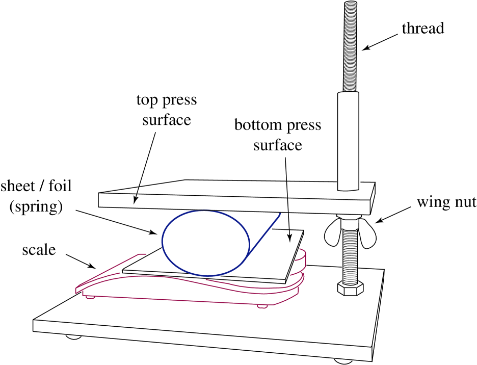
Figure 1: An illustration of the experimental setup.

The process of measurement can be setup so to start from a point where the top press surface barely touches the spring - this can be checked by the mass reading on the scale which must remain zero. The height of the unladen spring ($2b_{0}$) should be measured at this point. As the wing nut is turned, the reading of the scale ($m_{e}$) should be recorded after each full turn of the nut. If needed, the readings can be recorded after quarter or a half turn or even after an arbitrary angle by mounting an angular scale above the nut which can be used to precisely determine the percentage of the turn. The smallest angular turns of the wing nut that we used were $\pi/3$. Since the pitch of the nut/thread is known, this measurement procedure (with determined $2b_{0}$) enables one to obtain many pairs of data, relating effective mass/force $m_{e}$ to the spring height $2b$.

IV Variational approach to determination of the shape of deformed cylindrical spring

It is of use to think of this system by turning it upside-down in a sort of gedanken experiment. One can thus recognize that the effective mass measured by the scale can be thought of as a mass that presses the spring from ”above” due to gravity (the mass of the spring being neglected here). This enables one to pose the physical problem of spring deformation as a minimization of energy. The two types of energies in the system are the gravitational energy of the effective mass and the elastic (bending) energy of the deformed spring. The shape that shall be adopted by the spring minimizes the total energy functional,

$${\cal E}=E_{p}+E_{el}=2m_{e}gb+\frac{\kappa}{2}\int_{S}K^{2}dS.$$ (4)

As already mentioned, the spring surface can be parametrized by the profile of its cross-section i.e. the closed curve ${\cal C}$ that defines it. In the language of variational calculus (see e.g. Ref. variational_general, ), of all the possible curves that have the given length (so that the spring is inextensible) and height of $2b$, the curve that shall actually be adopted by the spring will be the one for which the functional in Eq. (4) is minimal. This statement can also be written as

$$\frac{\delta{\cal E}}{\delta{\cal C}}=0,$$ (5)

where the combination $\delta/\delta{\cal C}$ symbolizes the variation of a functional ${\cal E}$ with respect to the curves ${\cal C}$. The problem is well posed in this way since the curve ${\cal C}$ can be written in a quite general fashion, so that the variation of the energy functional produces differential equation for the function parametrizing the curve (the Euler-Lagrange equations) variational_general . However, such procedure typically results in equations that can be solved only numerically. Therefore, we resort to a simpler version of a variational approach that shall yield important analytical insights, however.

Instead of varying the functional ${\cal E}$ over all possible functions that represent ${\cal C}$, we can vary it over a particular subset of all functions. The subset that is chosen typically consists of functions that can be studied analytically and parametrized using small number of parameters whose variation spans the space of subset functions. A typical example of such procedure is a variational determination of the ground state energy of hydrogen atom that is studied in many textbooks (see e.g. Ref. Schiff, ). In our case, we must choose the functions that are (i) closed, (ii) produce a given circumference of the spring profile, and (iii) are confined to a space between the two press surfaces, so that the profile height is $2b$. There are two substantially different categories of functions that may be tested as variational solutions to the cross-section of the deformed cylindrical sheet. The functions in the first category touch the upper and lower press cross-sections in single points. A typical representative of such functions is an ellipse. The functions in the second category touch the upper and lower press cross-sections along the lines of certain length. A typical representative of such functions is the function made of two semi-circles connected by lines whose length corresponds to the separation of the centers of the semi-circles. In the further, we shall term this profile as the stadium, since the same name is used in the literature on quantum and classical chaos for the so-called billiards of such a shape (sometimes also the Bunimovich stadium after the researcher who studied it chaos_billiards ).

That the two types of functions really exist as solutions to the real problem can be checked experimentally by using our setup. Profiles quite similar to the stadium are obtained in case of cylinder that is laden with sufficient mass. The profiles from the first category appear for quite small loads (effective masses), and it may be somewhat difficult to judge whether the rolled sheet touches the press surfaces only tangentially or along a region of finite area. In any case, one should remember that the profiles are variational functions and they thus only mimic the true solution. For example, the stadium profile may mimic a solution whose curvature is very low in the regions where the profile almost touches the press surfaces and it becomes large in the two regions where the profile separates from the press surface. Such a profile may in fact touch the press surfaces (that become lines in the plane of the cross-section) only in four points, yet the stadium approximation should still be an adequate variational try (or ansatz as it is sometimes called in the professional literature). One should keep in mind, however, that, since the subset of variational functions is a restricted one, the energy that is obtained is an upper limit for the exact energy of the system, as is always the case in a variational approach variational_general ; Schiff .

In the following two subsections we shall solve the variational problem for the two categories of spring cross-sections.

IV.1 Stadium profile

The elastic energy of the stadium can be represented analytically by evaluating Eq. (2) for the profile. Flat pieces of the profile contribute nothing to the energy and the energy of the curved parts is easily calculated since these are two halves of a cylinder of height $h$ and radius $b$ (note that the curvature of the profile shows a discontinuity along the lines where the flat pieces meet the cylindrical ones). The two principal curvatures along the cylindrical portions are constant and given as $K_{1}=b^{-1}$, $K_{2}=0$ (since the radius of curvature along the cylinder height is infinite). The mean curvature is $K_{M}=b^{-1}/2$ ($K=b^{-1}$), so that the elastic energy is

$$E_{el}=\frac{\kappa}{2}\frac{2b\pi h}{b^{2}}=\frac{\pi\kappa h}{b}.$$ (6)

The total energy of the system for the chosen profile is now

$${\cal E}=2m_{e}gb+\frac{\pi\kappa h}{b}.$$ (7)

Requiring that for given effective load $m_{e}$, the total energy be minimal leaves us with a simple variational condition on $b$, which is the only parameter of the profile:

$$\frac{\partial{\cal E}}{\partial b}=2m_{e}g-\frac{\pi\kappa h}{b^{2}}\equiv 0.$$ (8)

This yields an equation for the profile characteristic radius (half of the height),

$$b=\sqrt{\frac{\kappa\pi h}{2m_{e}g}}.$$ (9)

Obviously, the above solution can be expected to be correct only for sufficiently large loads $m_{e}$, as it diverges as $m_{e}^{-1/2}$ when $m_{e}\to 0$. A more careful analysis would require that the maximally allowed value for $b$ be bounded from above by $b_{0}$, i.e. the radius of the cylinder in its unladen state - this is a form of the nonextensibility requirement to the solution. This yields an inequality that defines a region of the applicability of the solution,

$$\sqrt{\frac{\kappa\pi h}{2m_{e}g}}<b_{0}.$$ (10)

The inextensibility condition is easily satisfied whenever $b<b_{0}$ since the length of the flat parts of the profile can be adjusted as needed, without the change in the profile elastic energy. Note, however, that the region of validity of the solution is likely to be smaller, since the stadium shape may not be the best possible variational ansatz throughout the region defined by Eq. (10).

IV.2 Elliptic profile

The calculation of the elastic energy of an elliptic profile requires somewhat more mathematics than in the stadium case. We parametrize the ellipse as $x=a\cos t$, $y=b\sin t$, where $a$ and $b$ are the major and the minor axes, respectively. The curvature of such a profile can be calculated as explained in the Appendix, which yields $K_{G}=0$, as before, and

$$K=\frac{ab}{(a^{2}\cos^{2}t+b^{2}\sin^{2}t)^{3/2}}.$$ (11)

Evaluation of the integral in Eq. (2) with such a curvature yields

$$E_{el}=\frac{2\kappa h}{3b}\left[2\left(1+\frac{b^{2}}{a^{2}}\right)\mathpzc{E}\left(\sqrt{1-\frac{a^{2}}{b^{2}}}\right)-\mathpzc{K}\left(\sqrt{1-\frac{a^{2}}{b^{2}}}\right)\right],$$ (12)

where $\mathpzc{K}$ and $\mathpzc{E}$ are complete elliptic integrals of the first and second kinds, respectively notation_el_int . The major and minor axes of the ellipse are connected via the condition of inextensibility of the sheet, so that the profile circumference always equals the circumference in the unladen state, when the radius of the cylinder is $b_{0}$. Equating the circumference of the ellipse with that of a circle (in the unladen state) yields

$$\mathpzc{E}\left(\sqrt{1-\frac{a^{2}}{b^{2}}}\right)=\frac{b_{0}\pi}{2b}.$$ (13)

The problem now reduces to varying Eq. (12), and at the same time requiring Eq. (13) to hold. Instead of dealing with such a problem and all the inconveniences stemming from the appearance of special functions, we shall use the physical insight which tells us that elliptic profiles are likely to be observed for small deformations, i.e. when $a\approx b$. In that case, we can use the Taylor expansions of the elliptic integralsWolfram to relate the major and minor axes as $a^{2}=4bb_{0}-3b^{2}$, and obtain the elastic energy as

$$\lim_{a\to b}E_{el}=\frac{\pi h\kappa}{b}\left[\frac{5(b_{0}/b)-4\left(b_{0}/b\right)^{2}-2}{3-4(b_{0}/b)}\right].$$ (14)

The above expression differs from the elastic energy of the stadium profile [Eq. (6)] by the multiplicative factor in square parentheses. Examination of this factor reveals that it is smaller than one in the interval $b\in[0.80b_{0},b_{0}]$, and it becomes larger than one when $b<0.80b_{0}$. Thus, the elastic energy of the elliptic profile is smaller from the one corresponding to the stadium profile for initial deformation of the cylindrical spring, but for sufficiently large deformations ($b<0.80b_{0}$), the stadium profile becomes more favorable energywise. Already at this point, we may suspect that the response of the spring will show two characteristic regimes separated at point where $b\approx 0.8b_{0}$.

The characteristic profile parameter $b$ can be again obtained by varying the total energy which, with Eq. (14), yields a polynomial equation of fitfh degree for $b$. However, since we are interested in the solutions of this equation only for small deformations, we may again use Taylor expansion, but this time around the point where $b=b_{0}$, which then yields

$$b=b_{0}-\frac{m_{e}gb_{0}^{3}}{7\pi h\kappa}.$$ (15)

V Numerical solution to the problem: Universal energetics of the spring deformation

The problem of interest to us can be solved numerically. This can be done in many different ways. Perhaps the simplest one, and the one that we applied, is to discretize the profile of the deformed spring in $N$ points and to reformulate the energy functional so that it becomes a function of the coordinates of these points. Such a function can then be minimized using various numerical algorithms intended for such purpose. We shall use a particular variant of the conjugate gradient minimization that was successfully applied previously in Refs. siber_nano_el, ; siber_cones, ; Siber_vir1, ; Siber_vir2, . The constraints of the inextensibility of the sheet and the impenetrability of the top and bottom press surfaces can be implemented by suplementing the elastic energy with an energy penalty for all configurations that violate the constraints. Such a method is common in numerical optimization with constraints (see e.g. Ref. Siber_vir1, ). All these details are not really essential for our purposes, and we only need to know that the highly reliable numerical solution of our problem can be obtained.

The solution can be scaled so that it becomes universal i.e. applicable to appropriately scaled measurements of springs, irrespective of their equilibrium radii, $b_{0}$, heights $h$, and bending rigidities, $\kappa$. Such a scaled solution depends only on an adimensional parametrization of the shape, and the energy scale appears only as a multiplicative factor, scaling the universal solution to the concrete case with given spring dimensions and bending rigidity. The adimensional parameter that uniquely determines the spring shape is $b/b_{0}$, and an appropriate scale of elastic energy is $\pi\kappa h/b_{0}$ (one could also use $\kappa h/b$, but it is more convenient to have a fixed scale of energy that does not change during the spring deformation). The energy-shape dependence can thus be written as

$$\frac{b_{0}}{\pi\kappa h}E_{el}={\cal U}\left(\frac{b}{b_{0}}\right)\equiv\overline{E}_{el},$$ (16)

where ${\cal U}\left(b/b_{0}\right)$ is the universal function characteristic for our problem [note in particular that Eqs. (6) and (12) are of this form]. The appropriately scaled energy (adimensional) is denoted by an overline ($\overline{E}_{el}$), as will be all the adimensional quantitites in the following.

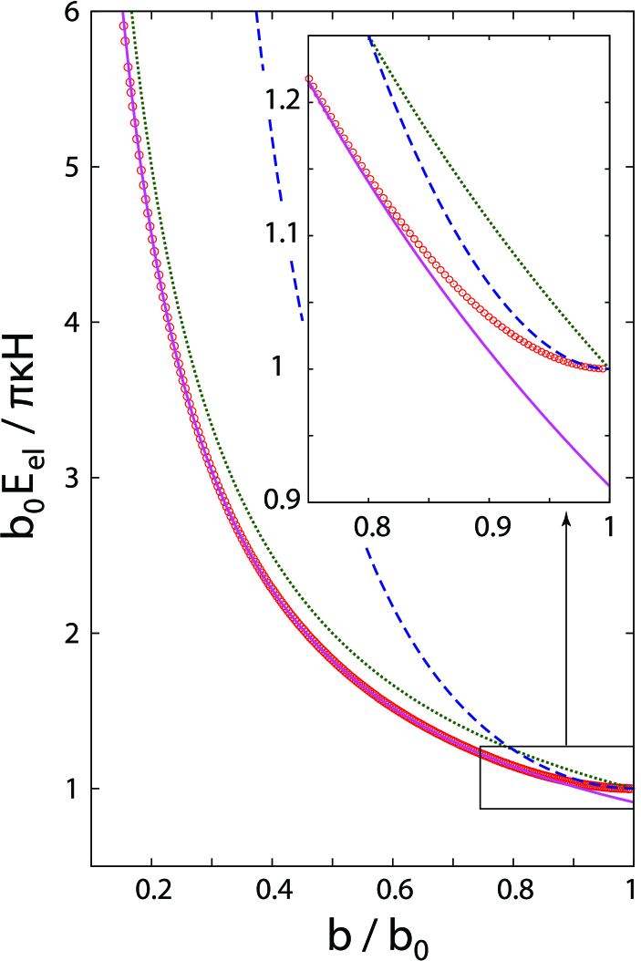
Figure 2: Theoretical predictions for the spring energies. The circles show the numerical results. The dotted line is the prediction of the variational method based on the stadium profile, Eq. (6). The dashed line is the variational prediction for the elliptical profile in the limit of small eccentricities, Eq. (14). The full line shows the scaled variational prediction of the stadium profile, obtained by a multiplication of the variational results (dotted line) by a factor of 0.912.

In Fig. 2 we show the theoretical predictions for the spring energy. The circles show the numerical data. The dotted line is the prediction of the variational method based on the stadium profile, Eq. (6). The dashed line is the variational prediction for the elliptical profile in the limit of small eccentricities, Eq. (14). We see that the variational prediction based on the stadium profile quite nicely follows the trend of the numerical (exact) results in the range when $b/b_{0}>0.7$, as expected from the discussion in the previous section. The variational energy is, however, always above the exact results, as is always the case in variational approach. However, a simple scaling of the energies obtained from stadium variational results by a factor of 0.912 gives a full line that fits the numerical data to a precision better than 0.8 % in the range $0.15<b/b_{0}<0.7$. One can immediately note the power of variational approach - although it may overestimate energies (by about 9 % in our case), it gives strong clues regarding functional behavior of energies that are not always easy to interpret solely from the numerical results. The stadium variational prediction becomes worse as $b>0.7b_{0}$, but the energies based on the elliptical profile are also quite unreliable in this interval, except quite close to the point where $b/b_{0}=1$. This was to be expected, having in mind the approximations that were used in deriving the variational prediction in Eq. (14), the assumption of small eccentricities in particular.

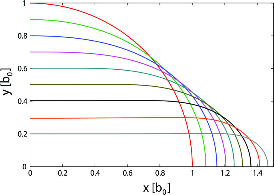
Figure 3: The spring profiles obtained by the numerical method. The compression parameters are $b/b_{0}$ = 1.0, 0.9, 0.8, 0.7, 0.6, 0.5, 0.4, 0.3, and 0.2 (from the highest to the lowest curve).

In Fig. 3, we show the profiles obtained by the numerical method. Only quarters of the profiles are shown as the remaining parts can be obtained by appropriate reflections about $x$ and $y$ axes. An astute reader may note a slight depression, concavity of the profile curve centered around $(x,y)=(0,b)$ point for sufficiently compressed springs ($b/b_{0}\lesssim 0.3$). This feature is also easily observed in experiments that we describe in the next section.

VI Experiment and theory: determining elastic properties of the sheet

In Fig. 4 we show four representative ”raw” experimental data, i.e. the half of the separation between the two press surfaces ($b$) as a function of the mass read on the scale ($m_{e}$). The measurements were performed on four different foils, all of them belonging to the same package. The thickness of the foils is nominally 200 $\mu$m, but our measurements of the average thickness of the foils in the package yielded 190 $\pm$ 7 $\mu$m. We shall denote these foils as belonging to the Set 1 in the following. We have rolled the foils along their longer side, so that $H=210$ mm. The separation between the two press surfaces just at the point where the foil barely touches the upper surface is $2b_{0}=92$ $\pm$ 1 mm. Note that $2b_{0}\pi=289$ mm which is 8 mm smaller from 297 mm (longer side of the A4 paper), and about half of this difference is due to small overlap of the foils that is necessary in order to apply the adhesive tape. The other half is due mostly to quite slight distortion of the foil under its own weight. We shall neglect this effect in the following, as we shall find no need for its inclusion in the data analysis.

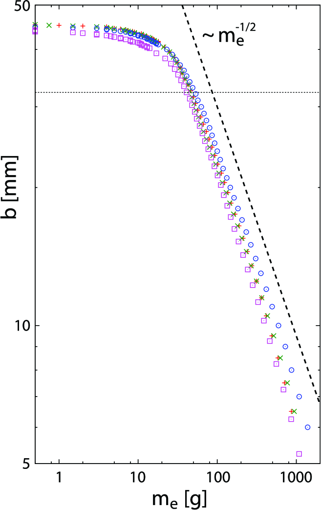
Figure 4: Four representative data sets (half of the spring height, $b$ vs. scale reading, $m_{e}$) obtained for four different foils marketed and sold as ”covers for binding, blue” with a thickness of 200 $\mu$m (Set 1). The foils were of A4 dimensions (210 $\times$ 297 mm) and we rolled them along the longer side in order to make a spring, thus $h=210$ mm. The dashed line shows the slope expected for the $b\propto m_{e}^{-1/2}$ dependence in the log-log representation. The thin dotted line shows $b=0.7\langle b_{0}\rangle$, where $\langle b_{0}\rangle$ is the average half-height of the spring in the unladen state for the four sets of data.

The dashed line in the figure shows the slope expected for $b\propto m_{e}^{-1/2}$ dependence in the stadium regime, as predicted by Eq. (9), but also by exact numerical solution shown in Fig. 2. One can see that the predicted dependence is nicely obeyed by the data below the dotted line that shows $b=0.7\langle b_{0}\rangle$, where $\langle b_{0}\rangle$ is the average half-height of the spring in the unladen state for the four sets of data. From the numerical analysis in the previous section, one finds that the easiest way to obtain the bending rigidity of the foils is to fit the experimental data to the

$$b=\sqrt{\frac{0.912\kappa\pi h}{2m_{e}g}}$$ (17)

dependence in the region $b<0.7b_{0}$. In addition to this, we shall perform a scaling analysis of the data, in accordance with the numerical results presented in Sec. V. The scaling analysis provides a universal description of the spring response, for all magnitudes of deformation and regardless of the spring bending rigidity, its height, and its unladen radius. It is thus of interest to experimentally investigate the predicted universality by studying differently shaped springs, and springs of different bending rigidities. It is easiest to analyze the scaling with respect to $h$, as the same sheet can be rolled either along its length/longer side (so that $h=W$), or along its width (so that $h=L$). Concerning the scaling with $\kappa$, it is not necessary that the springs be of different materials, as $\kappa$ scales with the sheet thickness as in Eq. (1), so that the sheets of the same material, but with different thicknesses are adequate in that respect. We have tested two additional sets of sheets, one of them sold again as binding covers (A4 format), but of smaller thickness (nominally 150 $\mu$m, but we measured 146 $\pm$ 8 $\mu$m). We denote the set of these foils by Set 2. Finally, the thickest set of sheets that we tested (A4 format, nominal thickness of 400 $\mu$m, but we measured 412 $\pm$ 4 $\mu$m) is marketed as ”flexible plastic film” and its intended purpose is to be used for cutting shapes out of it (we bought it in a hobby store). The set of these foils is denoted by Set 3.

For all the measurements we performed, we scaled the mass readings, so to produce the adimensional experimental force $\overline{F}_{exp}$ as

$$\overline{F}_{exp}=\frac{2m_{e}gb_{0}^{2}}{\pi\kappa h}.$$ (18)

The scale of force can be derived from the scale of energy, $\pi\kappa h/b_{0}$, simply by dividing it by the scale of length, $b_{0}$ in our case. The quantity in equation (18) can be directly compared to its counterpart obtained from the numerical analysis,

$$\overline{F}_{num}=-\frac{d\overline{E}_{el}}{d(b/b_{0})}.$$ (19)

Note that the factor of $2$ in Eq. (18) arises from the fact that compression of the spring where $b$ changes by $\Delta b$ requires applying the force of $m_{e}g$ on a distance of $2\Delta b$ - the same factor of $2$ is present in Eq. (4). The comparison of the scaled experimental readings with the numerical results is shown in Fig. 5. One can see that the scaling predicted by the numerical results is evident in the experimental data through an interval of almost four order of magnitude of the force ($y$-axis; in our experimental setup, this corresponds to effective masses from about a gram to several kilograms). Note also that experimental data confirm the numerical predictions through the whole interval of deformation, in the regime where the profile can be described as a stadium, but also in the regime of small deformations, where the stadium ansatz fails.

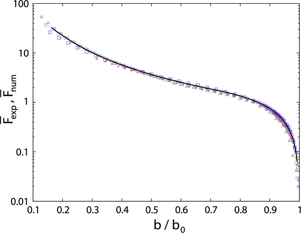
Figure 5: Scaled forces as specified by Eqs. (19) (line) and (18) (symbols). Circles and x-es are two representative data sets corresponding to the two sheets from Set 1 rolled along the longer and shorter sides, respectively. Triangles and squares are two representative data sets corresponding to the two sheets from Set 2 rolled along the longer and shorter sides, respectively. Pluses show a representative data set obtained from a representative measurement on a sheet from Set 3 rolled along its longer side. The full line shows the numerical results.

The summary of the bending rigidities obtained for the sheets shown in Fig. 5 is shown in Table 1. The fifth column of data contains the bulk Young modulus ($E$) of the sheets obtained from Eq. (1), using a value of $\kappa$ determined in the experiments and Poisson ratio of $\nu=0.3$ that is typical for most materials. The bulk Young moduli are indeed in the range expected for polymeric materials such as nylon, for example ($E\sim$ 2-4 GPa). One should note, though, that this analysis is approximate as we did not measure the Poisson ratio of the sheets.

Sheet	$h$ [cm]	$d$ [$\mu$m]	$\kappa$ [mJ]	$E$ [GPa]
Set 1	29.7	190	1.58	2.52
Set 1	21.0	190	1.59	2.53
Set 2	29.7	146	0.87	3.05
Set 2	21.0	146	0.71	2.48
Set 3	21.0	412	13.2	2.06

Table 1: Summary of the properties of the sheets we used in experiments shown in Fig. 5. The fourth and fifth columns of data were calculated as explained in the text.

This completes our theoretical and experimental analysis of the response of a thin cylindrical tube used as a spring.

VII Energy, elasticity, and deformation of thin shells in nano- and bio-systems

Sheet-like materials and shells made of them are not uncommon at the micro- and nano-scale. These structures are often theoretically studied using simplified variants of theory of elasticity elasticity_bio_nano , some of which are close to the one we presented. Here we mention several examples of recent research that can be understood in the context of physics that we presented in this work.

VII.1 Graphene, fullerenes, carbon nanotubes, graphene cones, …

An example of considerable recent interest is graphene - a single layer of carbon atoms in honeycomb arrangement graphene_rev . It is interesting that other single-shell carbon structures, such as fullerenes and carbon nanotubes carbon_nanotube_rev , can also be thought of as nanoscopic pieces of graphene material, cut-out from an infinite graphene plane in certain way and rolled and ”glued together” tersoff_1 ; carbon_nanotube_rev . With more elaborate cutting patterns, one can construct more complicated structures made of graphene, such as closed carbon cages, including fullerenes siber_nano_el and carbon/graphene cones siber_cones . Interestingly, it seems that one can calculate the energy of the structure, with respect to the energy of a planar piece of graphene, by accounting only for bending elastic energy of the shape in combination with the energy required to form pentagons in fullerenes, closed carbon nanotubes or carbon cones tersoff_1 ; siber_nano_el ; siber_cones . This is due to the fact that the shapes of these structures are locally pieces of cones and cylinders, so that the assumption of inextensibility holds ($K_{G}=0$). It is interesting that completely classical theory of elasticity can be succesfully applied to shapes in nano-domain (diameters of cylinders and shells $\sim$ 2 nm), but one should keep in mind that the bending rigidity parameter of graphene is determined by quantum physics - to calculate $\kappa$ for graphene, one should in principle account for change in energies of electrons in graphene that occurs when the planar piece of graphene is bent.

Not only the equilibrium shape and energy, but also deformation of nanotubes and fullerenes, can be studied using the theory of elasticity. For example in Ref. cnt_hydrostatic, , the deformation of carbon nanotubes under hydrostatic pressure is studied using a variational approach similar to ours, but with more complicated and versatile profiles. This is a problem somewhat different from the one we presented, nevertheless, shapes of deformed cylinders/nanotubes quite similar to ours (Fig. 3) were obtained.

VII.2 Viruses and microtubules

Biological systems abound with different structures whose characteristic dimensions are $\sim$ 10 nm. These are typically the so-called protein quaternary structures in which many proteins arrange in precise ways to form a larger shape. The quaternary structures often look like cylinders and shells of other geometries. Some typical examples are microtubules and protein coatings of certain viruses, such as tobacco mosaic virus. These structures are hollow cylinders made of many identical proteins. A different type of symmetry is more common in case of viruses - protein coatings of large number of viruses look like more or less spherical shells. The symmetry of such structures is quite similar to those of the icosahedral fullerenes, and analogous to pentagons and hexagons in fullerenes, the protein coatings of viruses are made of clusters of five and six proteins.

Energetics and elastic response of viruses and microtubules has been studied in the literature using various simplifications of the theory of elasticity LMN ; Siber_vir1 ; Siber_vir2 ; microtubule1 , some of which are similar to the one we presented. The experimental studies of such structures are typically performed using atomic force microscope (AFM) to press these structures against the substrate, which is an approach quite similar in spirit to the one we described. Such measurements yield information on the elastic response that can sometimes be difficult to interpret. In particular, when such experiments are used to measure the response of protein cylinders (tobacco mosaic virus or microtubule), the deformation depends also on the size of the AFM tip microtubule1 ; virus_AFM . In such case, the energy of stretching may become of importance in determining the overall deformation. In some cases, the shells of interest cannot be treated as thin.

VII.3 Vesicles

Vesicles are closed structures of different geometries formed by a sheet-like material that is usually a molecular bilayer. The typical diameters of vesicles are on the scale of micrometers Seifert97 ; Helfrich_original , and due to this fact, some consider them to represent a model system for cells membranes. In some cases, these structures can also be investigated by the AFM technique, especially when they are coated with proteins. Such problems are often solved variationally, using methods similar to those we used in our problem clathrin_vesicles .

*

Appendix A Curvatures of plane curves and surfaces

Differential geometry is a part of mathematics that deals with curvatures of plane and space curves and surfaces. For our purposes, we shall introduce only the most elementary notions, that are sufficient to mathematically support the physics of our problem. Somewhat more general views on surface curvatures are also summarized in Ref. Seifert97, .

A.1 Curvature of surfaces

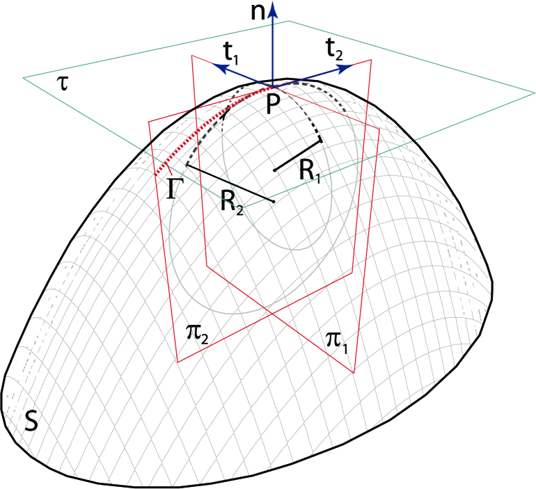
Figure 6: A sketch illustrating concepts relating to curvature of surfaces. Normal vector at point $P$ of the surface $S$ is denoted by ${\bf n}$, the tangential plane at $P$ is denoted by $\tau$, two tangential vectors in the two principal directions are denoted by ${\bf t}_{1}$ and ${\bf t}_{2}$, and the principal radii of curvature by $R_{1}$ and $R_{2}$. The two principal osculating circles are indicated by thick dashed lines. Curve $\Gamma$ is obtained as intersection of the surface $S$ and the plane $\pi_{2}$ that contains normal vector ${\bf n}$ and tangential direction vector ${\bf t}_{2}$.

Here we briefly introduce the basic concepts needed to define the curvature of surfaces. These are illustrated in Fig. 6. The normal vector at point $P$ of the surface $S$ is ${\bf n}$. The tangent plane $\tau$ at $P$ contains all the tangent vectors ${\bf t}$ perpendicular to ${\bf n}$. The intersection of a plane $\pi$ that contains ${\bf n}$ and a particular tangent vector ${\bf t}$ with a surface $S$ is a certain curve, $\Gamma$. This curve can be approximated by a circle around point $P$, so that (i) the circle passes through point $P$, (ii) the circle and the curve $\Gamma$ have a common tangent line at $P$, and (iii) the distance between the points the circle and on curve $\Gamma$ in the normal direction ${\bf n}$ decays as the cube of a higher power of the distance of these points to $P$ in the tangential direction ${\bf t}$. Such a circle is called the osculating circle of a curve $\Gamma$ (in direction ${\bf t}$). The minimum ($R_{1}$) and maximum ($R_{2}$) radii of all possible osculating circles at point $P$ (in all possible tangential directions) are called the principal radii of curvature. The two (principal) osculating circles belong to mutually perpendicular planes. The principal curvatures at point $P$ are given as $K_{1}\equiv R_{1}^{-1}$ and $K_{2}\equiv R_{2}^{-1}$.

The mean ($K_{M}$) and gaussian ($K_{G}$) curvatures at point $P$ are defined as

$$K_{M} = \frac{K_{1}+K_{2}}{2}$$

$$K_{G} = K_{1}K_{2}$$ (20)

We define

$$K\equiv 2K_{M}=K_{1}+K_{2},$$ (21)

i.e. twice the mean curvature.

A.2 Curvature of plane curves

The curvature of a plane curve given in a parametric form, $x=x(t)$, $y=y(t)$ can be obtained as

$$K_{1}=\frac{x^{\prime}y^{\prime\prime}-y^{\prime}x^{\prime\prime}}{\left(x^{\prime 2}+y^{\prime 2}\right)^{3/2}},$$ (22)

where $x^{\prime}\equiv dx/dt$, $y^{\prime}\equiv dy/dt$.

References

- (1) Stephen P. Timoshenko and James P. Gere, Theory of elastic stability (McGraw-Hill International, 1963), 2nd. ed. - international student edition.
- (2) Lee A. Segel, Mathematics applied to continuum mechanics, (Dover Publications, 1987).
- (3) Leonard I. Schiff, Quantum mechanics (McGraw-Hill, Singapore, 1968), 3rd. ed.
- (4) L.A. Bunimovich, “On the ergodic properties of nowhere dispersing billiards”, Comm. Math. Phys. 65, 295–312 (1979).
- (5) Wolfram Research, Inc., Mathematica Edition: Version 7.0 (Wolfram Research, Inc., Champaign, Illinois, 2008).
- (6) There are different notational conventions regarding the elliptic integrals. In our case, and .
- (7) A. Šiber, “Energies of sp2 carbon shapes with pentagonal disclinations and elasticity theory”, Nanotechnology 17, 3598 -3606 (2006).
- (8) A. Šiber, “Continuum and all-atom description of the energetics of graphene nanocones”, Nanotechnology 18, 375705-1–375705-6 (2007).
- (9) A. Šiber, “Buckling transition in icosahedral shells subjected to volume conservation constraint and pressure: Relations to virus maturation”, Phys. Rev. E 73, 061915-1–061915-10 (2006).
- (10) A. Šiber and R. Podgornik, “Stability of elastic icosadeltahedral shells under uniform external pressure: Application to viruses under osmotic pressure”, Phys. Rev. E 79, 011919-1-011919-5 (2009).
- (11) Z. C. Tu and Z. C. Ou-Yang, “Elastic theory of low-dimensional continua and its applications in bio- and nano-structures”, J. Comput. Theor. Nanosci. 5, 422 448 (2008).
- (12) C. Lee, X. Wei, J. W. Kysar, and J. Hone, “Measurement of the elastic properties and intrinsic strength of monolayer graphene”, Science 321, 385-388 (2008).
- (13) M.S. Dresselhaus, G. Dresselhaus, and Ph. Avouris (eds.), Carbon nanotubes: Synthesis, structure, properties, and applications (Springer-Verlag, Berlin, Heidelberg, 2001).
- (14) J. Tersoff, “Energies of fullerenes”, Phys. Rev. B 46, 15546–15549 (1992).
- (15) M. Hasegawa and K. Nishidate, “Radial deformation and stability of single-wall carbon nanotubes under hydrostatic pressure”, Phys. Rev. B 74, 115401-1–115401-10 (2006).
- (16) J. Lidmar, L. Mirny and D.R. Nelson, “Virus shapes and buckling transitions in spherical shells”, Phys. Rev. E 68, 051910-1–051910-10 (2003).
- (17) P. J. de Pablo, I. A.T. Schaap, F. C. MacKintosh, and C. F. Schmidt, “Deformation and collapse of microtubules on the nanometer scale”, Phys. Rev. Lett. 91, 098101-1–098101-4 (2003).
- (18) Y. Zhao, Z. Ge and J. Fang, “Elastic modulus of viral nanotubes”, Phys. Rev. E 78, 031914-1–031914-5 (2008).
- (19) U. Seifert, “Configurations of fluid membranes and vesicles”, Adv. Phys. 46, 13–137 (1997).
- (20) W. Helfrich, “Elastic properties of lipid bilayers: theory and possible experiments”, Z. Naturforsch. 28 c, 693–703 (1973).
- (21) A. J. Jin,K. Prasad, P. D. Smith, E. M. Lafer, and R. Nossal, “Measuring the elasticity of clathrin-coated vesicles via atomic force microscopy”, Biophys. J. 90, 3333–3344 (2006).