Linear problems and Bäcklund transformations for the Hirota-Ohta system

Abstract

The auxiliary linear problems are presented for all discretization levels of the Hirota-Ohta system. The structure of these linear problems coincides essentially with the structure of Nonlinear Schrödinger hierarchy. The squared eigenfunction constraints are found which relate Hirota-Ohta and Kulish-Sklyanin vectorial NLS hierarchies.

Key words: auxiliary linear problem, Bäcklund transformation, discretization

1 Introduction

The Hirota-Ohta system [13] was introduced by means of Pfaffianization applied to the Kadomtsev-Petviashvili equation, that is as a result of a certain procedure which allows to replace multi-soliton solutions represented by determinants with solutions represented by Pfaffians. Later on, this procedure was applied to many other equations, see e.g. [10]. The differential-difference member of the Hirota-Ohta hierarchy known as the Pfaff lattice [1, 2, 3, 16] was introduced within the theory of random matrix models. The whole hierarchy can be derived also within the general approach based on Clifford algebra representations and the boson-fermion correspondence [14, 15], for example, this technique was used for the derivation of Bäcklund transformation [20].

In this Letter we suggest an alternative and more simple derivation of the Hirota-Ohta hierarchy by use of Zakharov-Shabat method [26] based on the study of auxiliary linear problems. To the best of our knowledge, such linear problems for the continuous part of the hierarchy appeared so far only in paper [17]. The completely discrete Hirota-Ohta system was found for the first time, apparently, in paper [12]. However, it is not clear from this work, whether this discrete system belongs to the Hirota-Ohta hierarchy or just serves as its discrete analog. In Section 3, we answer in the affirmative to this question and provide the consistent linear problems for all discrete levels of the Hirota-Ohta system, that is for the systems with one, two and three discrete variables.

The linear problems under consideration are rather deep reductions. For example, in the completely discrete case, we consider a 2-component 4-point scheme with three field variables only, while the generic scheme of such type corresponding to the discrete Darboux-Zakharov-Manakov system [22, 7] contains eight fields (two $2\times 2$ matrices). The following empirical observation allows to recognize these reductions:

the structure of linear problems for 3-dimensional Hirota-Ohta hierarchy coincides with the structure of 2-dimensional hierarchy of Nonlinear Schrödinger equation (NLS).

The difference is that the nonlinear terms are replaced with the linear ones with variable coefficients, the Hirota-Ohta hierarchy arising from the compatibility conditions for these coefficients while the NLS flows commute identically.

In Section 2 we recall some standard equations from the NLS hierarchy: the third order higher symmetry, Bäcklund transformations and the nonlinear superposition principle. These equations are used as a hint while choosing the form of the linear problems for the Hirota-Ohta hierarchy in Section 3. A more precise conformity with the theory of 2-dimensional systems is pointed out in Section 4 devoted to the vectorial generalization of NLS by Kulish and Skkyanin [19]. This correspondence was found in [5] by one of the authors unaware of Hirota-Ohta results at that moment.

2 NLS hierarchy

The following notations are used below. The field variables $\psi,\phi$ depend on the infinite set of independent continuous variables $t_{1}=x$, $t_{2}=y$, $t_{3}=t,\dots$ and integer-valued variables $n_{1},\dots,n_{i},\dots,n_{j},\dots,n_{k},\dots$. Subscripts $x,y,t$ denote the partial derivatives, and subscripts $1,i,j,k$ denote the shifts on the discrete variables: $\psi_{i}=\psi(\dots,n_{i}+1,\dots)$, minus sign denoting the backward shift: $\psi_{-i}=\psi(\dots,n_{i}-1,\dots)$.

The Nonlinear Schrödinger equation is of the form

$$\psi_{y}=\psi_{xx}+2\psi^{2}\phi,\quad-\phi_{y}=\phi_{xx}+2\phi^{2}\psi.$$ (1)

Its simplest higher symmetry is of third order:

$$\psi_{t}=\psi_{xxx}+6\phi\psi\psi_{x},\quad\phi_{t}=\phi_{xxx}+6\psi\phi\phi_{x}.$$ (2)

The discrete variable $n_{1}$ will play the distinguished role in what follows. The corresponding shift defines Bäcklund-Schlesinger transformation as the explicit mapping

$$\psi_{1}=\psi_{xx}-\psi^{2}_{x}/\psi+\psi^{2}\phi,\quad\phi_{1}=1/\psi$$ (3)

which acts on the solutions of systems (1), (2). The iterations of this mapping are governed, under the change $\psi=e^{q}$, $\phi=e^{-q_{-1}}$, by the Toda lattice

$$q_{xx}=e^{q_{1}-q}-e^{q-q_{-1}}.$$ (4)

All other discrete variables correspond to Bäcklund-Darboux transformations; $x$-parts of these transformations are of the form

$$\psi_{x}=\psi_{i}+\alpha^{(i)}\psi+\psi^{2}\phi_{i},\quad-\phi_{i,x}=\phi+\alpha^{(i)}\phi_{i}+\phi^{2}_{i}\psi,$$ (5)

where $\alpha^{(i)}$ is an arbitrary parameter, associated with $i$-th discrete coordinate direction and depending on $n_{i}$ only (that is, $\alpha^{(i)}_{j}=\alpha^{(i)}$ at $j\neq i$). Second equation (5) defines $\phi_{i}$ as a solution of Riccati equation, then $\psi_{i}$ is explicitly found from the first equation. A generic Bäcklund transformation for the NLS equation is decomposed as a sequence of elementary transformations of the form (3), (5) and their inverses.

The completely discrete part of the NLS hierarchy is described by 5-point equations of discrete Toda type

$$e^{q_{1,-i}-q}-e^{q-q_{-1,i}}+e^{q_{i}-q}-e^{q-q_{-i}}+\alpha^{(i)}-\alpha^{(i)}_{-i}=0$$ (6)

and 2-component quad-equations

$$\psi_{j}=\psi_{i}+\frac{(\alpha^{(i)}-\alpha^{(j)})\psi}{1-\psi\phi_{ij}},\quad\phi_{j}=\phi_{i}+\frac{(\alpha^{(j)}-\alpha^{(i)})\phi_{ij}}{1-\psi\phi_{ij}}.$$ (7)

Equations (6) define the permutability property of the transformations (3) and (5). This means that equation (6) is consistent with the differentiation

$$q_{x}=e^{q_{i}-q}+e^{q-q_{-1,i}}+\alpha^{(i)}=e^{q_{1,-i}-q}+e^{q-q_{-i}}+\alpha^{(i)}_{-i},$$

that is the derivative with respect to $x$ of the left-hand side of (6) vanishes in virtue of (6) itself. Moreover, the variables $q(n_{1},n_{i})$ at fixed $n_{i}$ satisfy the Toda lattice (4), and variables $\psi=e^{q(n_{1},n_{i})}$, $\phi=e^{-q(n_{1}-1,n_{i})}$ at fixed $n_{1}$ satisfy the lattice (5).

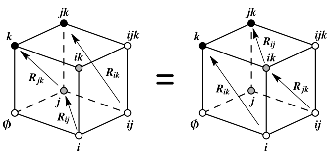
Figure 1: $R_{jk}R_{ik}R_{ij}=R_{ij}R_{ik}R_{jk}$

Analogously, equations (7) define the permutability property of two transformations of the form (5). Let $\Psi=(\psi,\phi)$, then the following property holds: if $\Psi$ and $\Psi_{i}$ are related by the transformation (5) with parameter $\alpha^{(i)}$, and $\Psi_{i}$ and $\Psi_{ij}$ are related by the transformation with parameter $\alpha^{(j)}$ then the variable $\Psi_{j}$ defined accordingly to (7) is as well related to $\Psi$ and $\Psi_{ij}$ by the transformations of the same type, but with the interchanged parameters $\alpha^{(j)}$ and $\alpha^{(i)}$.

The mappings $R_{ij}:(\Psi,\Psi_{i},\Psi_{ij})\mapsto\Psi_{j}$ satisfy an important 3D-consistency property expressed by the Yang-Baxter identity (see fig. 1)

$$R_{jk}R_{ik}R_{ij}=R_{ij}R_{ik}R_{jk}.$$ (8)

An essential distinction with the scalar quad-equations [6] is that equations (7) cannot be solved with respect to variables $\Psi$ or $\Psi_{ij}$. Hence the formulation of 3D-consistency is possible here only under a choice of the initial data along some sequence of the vertices of the cube, for example $\Psi$, $\Psi_{1}$, $\Psi_{12}$, $\Psi_{123}$.

3 Hirota-Ohta hierarchy

We keep the previous notations for the derivatives and shifts with respect to the independent variables. As for the dependent variables, now $\psi$ and $\phi$ play the role of wave-functions, while the field variables will be denoted $u,v$, $w,w^{(i)},w^{(ij)},q$ (coefficients of linear problems) and $f,g,h$ ($\tau$-functions). Superscripts in $w^{(i)}$, $w^{(ij)}$ indicate that these variables are associated with the corresponding direction or plane in the lattice (but, in contrast to parameters $\alpha^{(i)}$ from the previous section, these depend on the whole set of independent variables).

We accept the following linearization of the NLS equation (1) as a starting point:

$$\psi_{y}=\psi_{xx}+w\psi+2u\phi,\quad-\phi_{y}=\phi_{xx}+2v\psi+w\phi.$$ (9)

Now, let us search for a commuting flow of the form

$$\psi_{t}=\psi_{xxx}+a\psi_{x}+b\psi+c\phi,\quad\phi_{t}=\phi_{xxx}+A\phi_{x}+B\psi+C\phi$$

with undetermined coefficients (that is, the cubic terms in (2) are replaced with the linear combination of the factors). An easy computation specifies the coefficients:

$$\psi_{t} =\psi_{xxx}+\frac{3}{2}w\psi_{x}+\frac{3}{4}(w_{x}+q)\psi+3u_{x}\phi,$$ (10)

$$\phi_{t} =\phi_{xxx}+\frac{3}{2}w\phi_{x}+\frac{3}{4}(w_{x}-q)\phi+3v_{x}\psi$$

and yields the compatibility conditions of equations (9) and (10) in the form of the following system:

$$-2u_{t} =u_{xxx}-3u_{xy}+3wu_{x}-3qu,$$ (11)

$$-2v_{t} =v_{xxx}+3v_{xy}+3wv_{x}+3qv,$$

$$4w_{t} =w_{xxx}-24(uv)_{x}+6ww_{x}+3q_{y},\quad q_{x}=w_{y}.$$

This is nothing but the Hirota-Ohta system [13]. It is clear that its higher symmetries can be derived quite analogously by use of the linear problems of higher order with respect to $\partial_{x}$; however, we will skip this.

The change of variables

$$u=\frac{f}{h},\quad v=\frac{g}{h},\quad w=2(\log h)_{xx},\quad q=2(\log h)_{xy}$$ (12)

brings the system (11) to the bilinear form

$$(2D_{t}-3D_{x}D_{y}+D^{3}_{x})f\cdot h=0,$$ (13)

$$(2D_{t}+3D_{x}D_{y}+D^{3}_{x})g\cdot h=0,$$

$$(4D_{x}D_{t}-3D^{2}_{y}-D^{4}_{x})h\cdot h+24fg=0$$

where $D_{z}a\cdot b=a_{z}b-ab_{z}$ denotes the Hirota operator. The variables $f,g,h$ are especially convenient for rewriting of the discrete dynamics.

It is natural to search for an analog of the transformation (3) in the form

$$\psi_{1}=a\psi_{xx}+b\psi_{x}+c\psi+d\phi,\qquad\phi_{1}=p\psi.$$

The answer is not unique, because of the gauge transformations

$$\psi=\alpha\mu(y)\tilde{\psi},\quad\phi=\frac{\beta}{\mu(y)}\tilde{\phi},\quad\tilde{u}=\frac{\beta}{\alpha\mu^{2}}u,\quad\tilde{v}=\frac{\alpha\mu^{2}}{\beta}v,\quad\tilde{w}=w-\frac{\mu_{y}}{\mu}$$

which leave invariant the form of basic linear problem (9). It is possible to fix some coefficients by use of these transformations and to choose the mapping in the following form:

$$\psi_{1}=\psi_{xx}-\frac{u_{x}}{u}\psi_{x}+\Bigl{(}w+\frac{u_{xx}-u_{y}}{2u}\Bigr{)}\psi+u\phi,\quad\phi_{1}=-\frac{1}{u}\psi.$$ (14)

Its action on the coefficients of the linear problems is described as follows.

Statement 1.

System (11) admits the explicit auto-transformation

$$\begin{gathered}u_{1}=u^{2}v+\frac{1}{2}(u_{x}w_{x}-uw_{y})+\frac{w}{u}(uu_{xx}-u^{2}_{x})+\frac{1}{4u}\bigl{(}uu_{yy}-u^{2}_{y}\\ -2uu_{xxy}+2u_{x}u_{xy}+uu_{xxxx}-2u_{x}u_{xxx}+u^{2}_{xx}\bigr{)},\\[4.30554pt] v_{1}=1/u,\qquad w_{1}=w+2(\log u)_{xx},\qquad q_{1}=q+2(\log u)_{xy}.\end{gathered}$$ (15)

The substitutions (12) reduce the last three equations in (15) to $h_{1}=f$, $g_{1}=h$, that is the iterations of this mapping generate the sequence

$$\dots\quad f=h(n_{1}+1),\quad h=h(n_{1}),\quad g=h(n_{1}-1)\quad\dots$$

Moreover, the first equation (15) is equivalent to the relation

$$4\Bigl{(}\frac{A}{h_{1}h}\Bigr{)}_{x}=\frac{B_{1}}{h_{1}^{2}}-\frac{B}{h^{2}},$$

where

$$A=(3D_{x}D_{y}-D^{3}_{x})h_{1}\cdot h,\quad B=(3D^{2}_{y}+D^{4}_{x})h\cdot h-24h_{1}h_{-1}.$$

This relation is not bilinear, however it turns into identity in virtue of the system (13) which takes the form (cf [1, 2, 3])

$$(2D_{t}-3D_{x}D_{y}+D^{3}_{x})h_{1}\cdot h=0,$$ (16)

$$(4D_{x}D_{t}-3D^{2}_{y}-D^{4}_{x})h\cdot h+24h_{1}h_{-1}=0.$$

Indeed, in virtue of these equations

$$\frac{A}{h_{1}h}=2r_{1}-2r,\quad\frac{B}{h^{2}}=8r_{x},\quad r=\frac{h_{t}}{h}.$$

Darboux-Bäcklund transformation is derived from the linear problem

$$\psi_{x}=\psi_{i}+w^{(i)}\psi+u\phi_{i},\quad-\phi_{i,x}=\phi+v_{i}\psi+w^{(i)}\phi_{i},$$ (17)

and an analog of the nonlinear superposition principle (7) is described by the linear problem

$$\psi_{j}=\psi_{i}+w^{(ij)}(\psi+u\phi_{ij}),\quad\phi_{j}=\phi_{i}-w^{(ij)}(v_{ij}\psi+\phi_{ij}),\quad i\leq j.$$ (18)

The compatibility conditions for these equations define all discrete levels of the Hirota-Ohta system. We write them in the bilinear form at once, since the equations for the coefficients are rather bulky. To do this we use the following relations, in addition to the substitutions (12):

$$w^{(i)}=\frac{h_{i,x}}{h_{i}}-\frac{h_{x}}{h},\quad w^{(ij)}=\frac{hh_{ij}}{h_{i}h_{j}}.$$ (19)

Statement 2.

The compatibility conditions for equations (9) and (17) yield the system

$$fh_{i,y}-f_{y}h_{i}+fh_{i,xx}-2f_{x}h_{i,x}+f_{xx}h_{i}-2f_{i}h =0,$$

$$hg_{i,y}-h_{y}g_{i}+hg_{i,xx}-2h_{x}g_{i,x}+h_{xx}g_{i}-2h_{i}g =0,$$

$$hh_{i,y}-h_{y}h_{i}-hh_{i,xx}+2h_{x}h_{i,x}-h_{xx}h_{i}+2fg_{i} =0;$$ (20)

the compatibility conditions of (18) and two equations of the form (17), corresponding to $i$ and $j$, bring to the system

$$fh_{ij,x}-f_{x}h_{ij} =f_{i}h_{j}-f_{j}h_{i},$$

$$hg_{ij,x}-h_{x}g_{ij} =h_{i}g_{j}-h_{j}g_{i},$$

$$h_{i}h_{j,x}-h_{i,x}h_{j} =fg_{ij}-hh_{ij},\quad i<j;$$ (21)

the compatibility conditions for three linear problems of the form (18), corresponding to $i,j$ and $k$, yield the system

$$fh_{ijk}-f_{i}h_{jk}+f_{j}h_{ik}-f_{k}h_{ij} =0,$$

$$hg_{ijk}-h_{i}g_{jk}+h_{j}g_{ik}-h_{k}g_{ij} =0,$$

$$fg_{ijk}-h_{i}h_{jk}+h_{j}h_{ik}-h_{k}h_{ij} =0,\quad i<j<k.$$ (22)

Equations (22) are nothing but the discrete version of the Hirota-Ohta system found in [12]. Let us explain its derivation in more details. Formally one may consider the linear problem of form (18) as a very special case of 4-point scheme for 2-component function $\Psi=(\psi,\phi)$. As in the case of the NLS equation, $\phi$ and $\psi_{ij}$ are not involved in the equations, and this dictates the following choice of the initial data needed for the computation of compatibility conditions: $\Psi,\Psi_{i},\Psi_{ij},\Psi_{ijk}$. For the sake of definiteness we will assume that $i<j<k$. Then the compatibility condition is expressed by Yang-Baxter equation (8) where $R_{ij}$ is the mapping $(\Psi,\Psi_{i},\Psi_{ij})\mapsto\Psi_{j}$ defined by equations (18). The computations use the following equations:

$$R_{ij}: \begin{array}[]{ll}\psi_{j}=\psi_{i}+w^{(ij)}(\psi+u\phi_{ij}),\\ \phi_{j}=\phi_{i}-w^{(ij)}(v_{ij}\psi+\phi_{ij}),\end{array} \begin{array}[]{ll}\psi_{jk}=\psi_{ik}+w^{(ij)}_{k}(\psi_{k}+u_{k}\phi_{ijk}),\\ \phi_{jk}=\phi_{ik}-w^{(ij)}_{k}(v_{ijk}\psi_{k}+\phi_{ijk}),\end{array}$$

$$R_{ik}: \begin{array}[]{ll}\psi_{jk}=\psi_{ij}+w^{(ik)}_{j}(\psi_{j}+u_{j}\phi_{ijk}),\\ \phi_{jk}=\phi_{ij}-w^{(ik)}_{j}(v_{ijk}\psi_{j}+\phi_{ijk}),\end{array} \begin{array}[]{ll}\psi_{k}=\psi_{i}+w^{(ik)}(\psi+u\phi_{ik}),\\ \phi_{k}=\phi_{i}-w^{(ik)}(v_{ik}\psi+\phi_{ik}),\end{array}$$

$$R_{jk}: \begin{array}[]{ll}\psi_{k}=\psi_{j}+w^{(jk)}(\psi+u\phi_{jk}),\\ \phi_{k}=\phi_{j}-w^{(jk)}(v_{jk}\psi+\phi_{jk}),\end{array} \begin{array}[]{ll}\psi_{ik}=\psi_{ij}+w^{(jk)}_{i}(\psi_{i}+u_{i}\phi_{ijk}),\\ \phi_{ik}=\phi_{ij}-w^{(jk)}_{i}(v_{ijk}\psi_{i}+\phi_{ijk}).\end{array}$$

Left hand side of Yang-Baxter equation (8) corresponds to the consecutive computations according to the left column downwards, while the right hand side corresponds to the right column computed upwards. The resulting nonlinear relations for the coefficients contain, in particular, the conservation laws which imply the parametrization of $w^{(ij)}$ given in (19). The rest relations then turn out to be equivalent to system (22).

4 Kulish-Sklyanin vector hierarchy

A wide and well-known class of reductions from 3-dimensional equations to vectorial 2-dimensional ones consists of so-called squared eigenfunction constraints. For instance, the Manakov system [21, 9] and its third order symmetry

$$\psi_{y}=\psi_{xx}+2\langle\psi,\phi\rangle\psi,\quad-\phi_{y}=\phi_{xx}+2\langle\psi,\phi\rangle\phi,$$

$$\psi_{t}=\psi_{xxx}+3\langle\psi,\phi\rangle\psi_{x}+3\langle\psi_{x},\phi\rangle\psi,\quad\phi_{t}=\phi_{xxx}+3\langle\psi,\phi\rangle\phi_{x}+3\langle\psi,\phi_{x}\rangle\phi$$

define such a reduction for the Kadomtsev-Petviashvili equation

$$4u_{t}=u_{xxx}-6uu_{x}+3q_{y},\quad q_{x}=u_{y}$$

with respect to the quantities $u=-2\langle\psi,\phi\rangle$, $q=2\langle\psi,\phi_{x}\rangle-2\langle\psi_{x},\phi\rangle$ [18].

Now we demonstrate that the Hirota-Ohta hierarchy (for all discrete levels) arises analogously from another vectorial version of the NLS equation introduced by Kulish and Sklyanin [19]:

$$\psi_{y} =\psi_{xx}+4\langle\psi,\phi\rangle\psi-2\langle\psi,\psi\rangle\phi,$$ (23)

$$-\phi_{y} =\phi_{xx}+4\langle\psi,\phi\rangle\phi-2\langle\phi,\phi\rangle\psi.$$

Let us write the corresponding generalizations for the basic equations in Section 2. The third order symmetry reads

$$\psi_{t} =\psi_{xxx}+6\langle\psi,\phi\rangle\psi_{x}+6\langle\psi_{x},\phi\rangle\psi-6\langle\psi,\psi_{x}\rangle\phi,$$ (24)

$$\phi_{t} =\phi_{xxx}+6\langle\psi,\phi\rangle\phi_{x}+6\langle\psi,\phi_{x}\rangle\phi-6\langle\phi,\phi_{x}\rangle\psi.$$

The analog of Bäcklund-Schlesinger transformation (3) is of the form [25]

$$\psi_{1} =\psi_{xx}-2\frac{\langle\psi,\psi_{x}\rangle}{\langle\psi,\psi\rangle}\psi_{x}+\frac{\langle\psi_{x},\psi_{x}\rangle}{\langle\psi,\psi\rangle}\psi+2\langle\psi,\phi\rangle\psi-\langle\psi,\psi\rangle\phi,$$ (25)

$$\phi_{1} =\frac{1}{\langle\psi,\psi\rangle}\psi,$$

the analog of Bäcklund-Darboux transformation (5) reads

$$\psi_{x} =\psi_{i}+\alpha^{(i)}\psi+2\langle\psi,\phi_{i}\rangle\psi-\langle\psi,\psi\rangle\phi_{i},$$ (26)

$$-\phi_{i,x} =\phi+\alpha^{(i)}\phi_{i}+2\langle\psi,\phi_{i}\rangle\phi_{i}-\langle\phi_{i},\phi_{i}\rangle\psi$$

and, finally, the analog of nonlinear superposition principle (7) is [4]

$$\psi_{j}=\psi_{i}+\frac{(\alpha^{(i)}-\alpha^{(j)})(\psi-\langle\psi,\psi\rangle\phi_{ij})}{1-2\langle\psi,\phi_{ij}\rangle+\langle\psi,\psi\rangle\langle\phi_{ij},\phi_{ij}\rangle},$$ (27)

$$\phi_{j}=\phi_{i}-\frac{(\alpha^{(i)}-\alpha^{(j)})(\phi_{ij}-\langle\phi_{ij},\phi_{ij}\rangle\psi)}{1-2\langle\psi,\phi_{ij}\rangle+\langle\psi,\psi\rangle\langle\phi_{ij},\phi_{ij}\rangle}.$$

The comparison with the linear problems from the previous section proves immediately that the Kulish-Sklyanin hierarchy is their self-consistent reduction. More precisely, the following statement holds true.

Statement 3.

Equations (23)–(27) are consistent and, in virtue of these equations, the quantities

$$u=-\langle\psi,\psi\rangle,\quad v=-\langle\phi,\phi\rangle,\quad w=4\langle\psi,\phi\rangle,\quad q=4\langle\psi_{x},\phi\rangle-4\langle\psi,\phi_{x}\rangle,$$

$$w^{(i)}=\alpha^{(i)}+2\langle\psi,\phi_{i}\rangle,\quad w^{(ij)}=\frac{\alpha^{(i)}-\alpha^{(j)}}{1-2\langle\psi,\phi_{ij}\rangle+\langle\psi,\psi\rangle\langle\phi_{ij},\phi_{ij}\rangle}$$

satisfy the equations of the Hirota-Ohta hierarchy.

5 Concluding remarks

The main result of this Letter is an uniform derivation of continuous and discrete equations of the Hirota-Ohta hierarchy from the compatibility conditions of auxiliary linear problems. The structure of these problems patterns after the structure of 2-dimensional NLS hierarchy. We hope that this observation may be useful for other 3-dimensional equations as well.

It is worth noticing also the relation of above discrete linear problems with self-adjoint 5- and 7-point schemes, on square and triangular lattices respectively. The linear problems of this type attracted much attention recently. In particular, it is known that they appear from the scalar 4-point schemes on square and rhombic lattices as a result of restriction on even/odd sublattices [8]. In our case, such linear problems appear from 2-component linear problems presented in Section 3 as a result of elimination of one component. For instance, the elimination of $\phi$ from (14) and (17) yields the following 5-point equation (compare with discrete Toda lattice (6)):

$$\frac{1}{u}\psi_{i}+\frac{1}{u_{-i}}\psi_{-i}-\frac{1}{u}\psi_{1,-i}-\frac{1}{u_{-1,i}}\psi_{-1,i}+\frac{1}{u}\Bigl{(}w^{(i)}_{1,-i}+w^{(i)}-\frac{u_{x}}{u}\Bigr{)}\psi=0.$$

Analogously, eliminating $\phi$ from equations (18) results in the 7-point linear problem in the plane $(ij)$. We mention that some examples of continuous Toda-like dynamics associated with 5- and 7-point linear problems were studied in the papers [24, 11, 23]. It remains unclear, whether these examples coincide with the flow (17) of the Hirota-Ohta hierarchy; more likely, they may interpreted as its negative flows.

Acknowledgements.

The research of V.A. was supported by RFBR grants 08-01-00453, 09-01-92431-KE and NSh-6501.2010.2.

References

- [1] M. Adler, E. Horozov, P. van Moerbeke. The Pfaff lattice and skew-orthogonal polynomials. Int. Math. Res. Notes 1999:11 (1999) 569–588.
- [2] M. Adler, P. van Moerbeke. Toda versus Pfaff lattice and related polynomials. Duke Math. J. 112:1 (2002) 1–58.
- [3] M. Adler, T. Shiota, P. van Moerbeke. Pfaff -functions. Math. Ann. 322 (2002) 423–476.
- [4] V.E. Adler. Nonlinear superposition formula for Jordan NLS equations. Phys. Lett. A 190 (1994) 53–58.
- [5] V.E. Adler. On the relation between multifield and multidimensional integrable equations. arXiv:nlin/0011039v1.
- [6] V.E. Adler, A.I. Bobenko, Yu.B. Suris. Classification of integrable equations on quad-graphs. The consistency approach. Comm. Math. Phys. 233 (2003) 513–543.
- [7] L.V. Bogdanov, B.G. Konopelchenko. Lattice and -difference Darboux-Zakharov-Manakov systems via -dressing method. J. Phys. A 28:5 (1995) L173–178.
- [8] A. Doliwa, M. Nieszporski, P.M. Santini. Integrable lattices and their sublattices. II. From the B-quadrilateral lattice to the self-adjoint schemes on the triangular and the honeycomb lattices. J. Math. Phys. 48 (2007) 113506.
- [9] A.P. Fordy, P.P. Kulish. Nonlinear Schrödinger equations and simple Lie algebras. Comm. Math. Phys. 89:3 (1983) 427–443.
- [10] C.R. Gilson. Generalizing the KP hierarchies: Pfaffian hierarchies. Theor. Math. Phys. 133:3 (2002) 1663–1674.
- [11] C.R. Gilson, J.J.C. Nimmo. The relation between a 2D Lotka-Volterra equation and a 2D Toda lattice. J. Nonl. Math. Phys. 12, Suppl. 2 (2005) 169–179.
- [12] C.R. Gilson, J.J.C. Nimmo, S. Tsujimoto. Pfaffianization of the discrete KP equation. J. Phys. A 34:48 (2001) 10569–10575.
- [13] R. Hirota, Y. Ohta. Hierarchies of coupled soliton equations. I. J. Phys. Soc. Japan 60 (1991) 798–809.
- [14] M. Jimbo, T. Miwa. Solitons and infinite dimensional Lie algebras. Publ. Res. Inst. Math. Sci. Kyoto University 19 (1983) 943–1001.
- [15] V.G. Kac, J.W. van de Leur. The geometry of spinors and the multicomponent BKP and DKP hierarchies. In “The bispectral problem”, eds J. Harnad, A. Kasman, CRM Proc. Lecture notes 14, AMS, Providence (1998) 159–202.
- [16] S. Kakei. Orthogonal and symplectic matrix integrals and coupled KP hierarchy. J. Phys. Soc. Japan 68 (1999) 2875–2877.
- [17] S. Kakei. Dressing method and the coupled KP hierarchy. Phys. Lett. A 264:6 (2000) 449–458.
- [18] B.G. Konopelchenko, J. Sidorenko, W. Strampp. (1+1)-dimensional integrable systems as symmetry constraints of (2+1)-dimensional systems. Phys. Lett. A 157:1 (1991) 17–21.
- [19] P.P. Kulish, E.K. Sklyanin. -invariant nonlinear Schrödinger equation — a new completely integrable system. Phys. Lett. A 84:7 (1981) 349–352.
- [20] J. van de Leur. Bäcklund-Darboux transformations for the coupled KP hierarchy. J. Phys. A 37 (2004) 4395–4405.
- [21] S.V. Manakov. On the theory of two-dimensional stationary self-focusing of electromagnetic waves. JETP 38:2 (1974) 248–253.
- [22] F.W. Nijhoff, H.W. Capel. The direct linearisation approach to hierarchies of integrable PDEs in dimensions: I. Lattice equations and the differential-difference hierarchies. Inverse Problems 6:4 (1990) 567–590.
- [23] P.M. Santini, A. Doliwa, M. Nieszporski. Integrable dynamics of Toda-type on the square and triangular lattices. Phys. Rev. E 77:5 (2008) 056601.
- [24] P.M. Santini, M. Nieszporski, A. Doliwa. An integrable generalization of the Toda law to the square lattice. Phys. Rev. E 70:5 (2004) 056615.
- [25] S.I. Svinolupov, R.I. Yamilov. Explicit Bäcklund transformations for multifield Schrödinger equations. Jordan generalizations of the Toda chain. Theor. Math. Phys. 98:2 (1994) 139–146.
- [26] V.E. Zakharov, A.B. Shabat. The scheme of integration of nonlinear equations of mathematical physics by inverse scattering method. I. Funct. An. Appl. 8:3 (1974) 226–235.