We investigate the photon emission from the electrosphere of a quark star. It is shown that at temperatures $T\sim 0.1\div 1$ MeV the dominating mechanism is the bremsstrahlung due to bending of electron trajectories in the mean Coulomb field of the electrosphere. The radiated energy for this mechanism is much larger than that for the Bethe-Heitler bremsstrahlung. The energy flux from the mean field bremsstrahlung exceeds the one from the tunnel $e^{+}e^{-}$ pair creation as well. We demonstrate that the LPM suppression of the photon emission is negligible.

1 Introduction

The hypothesis of quark stars made of a stable strange quark matter (SQM) [1, 2, 3] has been attracting much attention for many years. It is possible that quark stars (if they exist) may be (at least in the initial hot stage) without a crust of normal matter [4]. Contrary to neutron stars the density of SQM for bare quark stars should drop abruptly at the scale $\sim 1$ fm. The SQM in normal phase and in the two-flavor superconducting (2SC) phase should also contain electrons (for normal phase the electron chemical potential, $\mu$, is about 20 MeV [2, 5]). In contrast to the quark density the electron density drops smoothly above the star surface at the scale $\sim 10^{3}$ fm [2, 5]. For the star surface temperature $T\ll\mu$, say $T\mathrel{\hbox to0.0pt{\lower 4.0pt\hbox{\hskip 1.0pt$\sim$}\hss}\raise 1.0pt\hbox{$<$}}10^{10}\mbox{K}\sim 1$ MeV, this “electron atmosphere” (usually called the electrosphere) may be viewed as a strongly degenerate relativistic electron gas [2, 5].

From the point of view of distinguishing bare quark stars from neutron stars it is of great importance to have theoretical predictions for the photon emission from bare quark stars. Contrary to neutron stars (or quark stars with a crust of normal matter) the photon emission from quark stars made of a stable self-bound SQM may potentially exceed the Eddington limit. This fact may be used for detecting a bare quark star. However, the SQM itself is a very poor emitter at $T\ll\omega_{p}^{q}$ [6, 7] (here $\omega_{p}^{q}\sim 20$ MeV is the plasma frequency of the SQM [6]). At such temperatures the photon emission from the quark surface is a tunnel process, and the radiation rate turns out to be negligibly small as compared to the black body radiation [6]. However, for the electrosphere the plasma frequency, $\omega_{p}^{e}$, is much smaller than that for the SQM. For this reason the photon emission from the electrosphere may potentially dominate the luminosity of a quark star. For understanding the prospect of detecting bare quark stars it is highly desirable to have quantitative predictions for the photon emission from the electrosphere. This is also of interest in the context of the scenario of the gamma-ray repeaters due to reheating of a quark star by impact of a massive comet-like object [8], and the dark matter model in the form of matter/antimatter SQM nuggets [9].

An obvious candidate for the photon emission from the electrosphere is the bremsstrahlung from electrons. It may be due to either the electron-electron interaction (the Bethe-Heitler bremsstrahlung) or interaction of electrons with the mean electric field of the electrosphere. One more mechanism is related to the tunnel $e^{+}e^{-}$ pair creation [4, 10]. The point is that the electric field of the electrosphere should be very strong. It may be about several tens of the critical field for the tunnel Schwinger pair production $E_{cr}=m_{e}^{2}/e$ [11] (we use units $c=\hbar=k_{B}=1$). In this scenario the photons appear through $e^{+}e^{-}$ annihilation in the outflowing $e^{\pm}$ wind [12].

The bremsstrahlung from the electrosphere due to the electron-electron interaction has been addressed in [13, 14]. The authors of [13] used the soft photon approximation and factorized the $e^{-}e^{-}\to e^{-}e^{-}$ cross section in the spirit of Low’s theorem. In [14] it was pointed out that this approximation is inadequate since it neglects the effect of the photon energy on the electron Pauli-blocking which should lead to a strong suppression of the radiation rate. The authors of [14] have not given a consistent treatment of this problem either. To take into account the effect of the minimal photon energy they suggested some restrictions on the initial electron momenta imposed by hand. In this way they obtained the radiated energy flux from the $e^{-}e^{-}\to e^{-}e^{-}\gamma$ process which is much smaller than that in [13], and than the energy flux from the tunnel $e^{+}e^{-}$ pair creation [4, 10]. In [15] there was an initial attempt to include the effect of the mean Coulomb field of the electrosphere on the photon emission. The authors obtained a considerable enhancement of the radiation rate. However, similarly to [13] the analysis [15] treats incorrectly the Pauli-blocking effect. Note also that in the analyses [14, 15] the photon quasiparticle mass was neglected. As we will show this approximation is clearly inadequate since the finite photon mass suppresses the radiation rate strongly.

Thus the theoretical situation with the photon bremsstrahlung from the electrosphere is still controversial and uncertain. The main problem here, which was not solved in the previous analyses [13, 14, 15], is an accurate accounting for the photon energy in the electron Pauli-blocking. In the present paper we address the bremsstrahlung from the electrosphere in a way similar to the Arnold-Moore-Yaffe (AMY) [16] approach to the collinear photon emission from a hot quark-gluon plasma based on the thermal field theory. We use a reformulation of the AMY formalism given in [17]. It is based on the light-cone path integral (LCPI) approach [18, 19, 20] (for reviews, see [21, 22]) to the in-medium radiation processes. For an infinite homogeneous plasma (with zero mean field) the formalism [17] reproduces the AMY results [16]. The LCPI formulation [17] has the advantage that it also works for plasmas with nonzero mean field. It allows to evaluate the photon emission accounting for bending of the electron trajectories in the mean Coulomb potential of the electrosphere. Contrary to very crude and qualitative methods of [13, 14, 15] the treatment of the Pauli-blocking effects in [16, 17] has robust quantum field theoretical grounds. Of course, our approach is only valid in the regime of collinear photon emission when the dominating photon energies exceed several units of the photon quasiparticle mass. Numerical calculations show that even at $T\sim 0.1$ MeV the effect of the noncollinear configurations is relatively small.

We demonstrate that for the temperatures $T\sim 0.1\div 1$ MeV the radiated energy flux from the $e^{-}\to e^{-}\gamma$ transition in the mean electric field turns out to be much larger than that from the Bethe-Heitler bremsstrahlung. It exceeds the energy flux from the tunnel $e^{+}e^{-}$ pairs as well. Also, we demonstrate that, contrary to conclusion of [13], the Landau-Pomeranchuk-Migdal (LPM) suppression [23, 24] of the photon bremsstrahlung is negligible. Our results show that the photon emission from the electrosphere may be of the same order as the black body radiation. For this reason the situation with distinguishing a bare quark star made of the SQM in normal (or 2SC) phase from a neutron star using the luminosity [4, 25] may be more optimistic than in the scenario with the tunnel $e^{+}e^{-}$ pair creation [4].

In a short version the results of this work were presented in [26]. In this paper we present our results in a more detailed form. The plan of the paper is as follows. In Sec. 2 we review the basic formulas and approximations. In Sec. 3 we discuss the evaluation of photon emission from a given electron in the electromagnetic field of the electrosphere which includes both the mean Coulomb field and the ordinary fluctuation field generated by neighboring electrons. In Sec. 4 we present numerical results for the radiated energy flux. Sec. 5 is devoted to conclusions.

2 Basic formulas and approximations

As in Refs. [4, 13, 14] we use for the electrosphere the model of a relativistic strongly degenerate electron gas in the Thomas-Fermi approximation. In this approximation the local electron number density reads $n_{e}(h)=\mu^{3}(h)/3\pi^{2}$, where $h$ is the distance from the quark surface. The $h$ dependence of the chemical potential is governed by the Poisson equation for the electrostatic potential $V=\mu/e$. For $h>0$ this gives [2, 5]

$$\mu(h)=\frac{\mu(0)}{(1+h/H)}\,,$$ (1)

where $H=\sqrt{{3\pi}/{2\alpha}}/\mu(0)$, $\alpha=e^{2}/4\pi$.

We assume that the electrosphere is optically thin. This means that the photon absorption and stimulated emission can be neglected. In this regime the luminosity may be expressed in terms of the energy radiated spontaneously per unit time and volume, $Q$, usually called the emissitivity. In the formalism [17] the emissitivity per unit photon energy $\omega$ at a given $h$ can be written as

$$\frac{dQ(h,\omega)}{d\omega}=\frac{\omega(k)}{4\pi^{3}}\frac{dk}{d\omega}\int\frac{d\mbox{{\bf p}}}{p}n_{F}(E)[1-n_{F}(E^{\prime})]\theta(p-k)\frac{dP(\mbox{{\bf p}},x)}{dxdL}\,,$$ (2)

where $k$ denotes the photon momentum, $E$ and $E^{\prime}$ are the electron energies before and after photon emission, $n_{F}(E)=[\exp((E-\mu)/T)+1]^{-1}$ is the local electron Fermi distribution (we omit the argument $h$ in the functions on the right-hand side of (2)), and $x=k/p$ is the photon longitudinal (along the initial electron momentum p) fractional momentum. The function $dP/dxdL$ in (2) is the probability of the photon emission per unit $x$ and length from an electron in the potential generated by other electrons which includes both the smooth collective Coulomb field and the usual fluctuating plasma part related to the field generated by the neighboring electrons. Note that the formula (2) accounts for photons emitted to all directions, because in the optically thin electrosphere practically all the photons radiated to the hemisphere directed to the quark surface will be reflected either in the electrosphere (at the level with $\omega_{p}^{e}=\omega$) or from the quark surface. Only the photons with $\omega\mathrel{\hbox to0.0pt{\lower 4.0pt\hbox{\hskip 1.0pt$\sim$}\hss}\raise 1.0pt\hbox{$>$}}\omega_{p}^{q}\sim 20$ MeV may be absorbed in the quark matter. However, such photons are not important at $T\mathrel{\hbox to0.0pt{\lower 4.0pt\hbox{\hskip 1.0pt$\sim$}\hss}\raise 1.0pt\hbox{$<$}}1$ MeV considered in the present paper. For the above reasons, it would be incorrect to exclude the photons emitted towards the star surface, as was done in [14].

Our basic formula (2) assumes that the photon emission is a local process, i.e. the photon formation length (we denote it $l_{f}$) is small compared to the thickness of the electrosphere. Evidently, only in this case one can define a local emissitivity. Note that Eq. (2) defines the rate of photon production at a given photon energy, which remains constant during the photon propagation in the electrosphere. The photon momentum in this process changes adiabatically according to the photon quasiparticle dispersion relation in the electron plasma. Also, the formula (2) assumes that on the scale $\sim l_{f}$ the electron trajectories are smooth. It means that besides the evident condition $l_{f}\ll R_{m}$ ($R_{m}$ is the radius of curvature of the electron trajectory in the mean field) the typical scattering angle related to the random walk of an electron due to electron-electron interaction should be small as well. One can show that these conditions are satisfied for the electrosphere. An important consequence of the smoothness of electron trajectories at the scale $\sim l_{f}$ is the longitudinal factorization of the Pauli-blocking factor $[1-n_{F}(E^{\prime})]$ for the final state of the radiating electron in (2). Namely the fact that the trajectories are smooth in the process of the photon emission allows one to neglect the statistics effects in treating the small angle scattering. Indeed, the typical space scale for the soft fluctuating modes of the electromagnetic field is about the inverse Debye mass $1/m_{D}\sim 1/e\mu$. This scale is much larger than the typical separation between electrons $\sim 1/\mu$. For this reason from the point of view of the electrons with energy $\sim\mu$ the soft electromagnetic field at the space scale $\sim 1/m_{D}\gg 1/\mu$ can be viewed as a uniform field at the scale $\sim 1/\mu$. In a uniform field all electrons in the same spin state scatter in the same way, and the small angle scattering leads simply to some shift of the distribution function in the momentum space. Any statistics effects will be suppressed by some power of electron charge $e$. Calculations within the real time thermal field theory performed in [16] corroborate this physical picture of the collinear photon emission.

In our approximation of optically thin medium the differential radiated energy flux from the electrosphere, $dF/d\omega$, in terms of the emissitivity reads

$$\frac{dF}{d\omega}=\int_{0}^{h_{max}}dh\frac{dQ(h,\omega)}{d\omega}\,.$$ (3)

For the chemical potential (1) the $h$-integration in (3) can be approximated by the integration over $\mu$ as

$$\frac{dF}{d\omega}\approx\sqrt{\frac{3\pi}{2\alpha}}\int_{\mu_{min}}^{\mu(0)}\frac{d\mu}{\mu^{2}}\frac{dQ(h(\mu),\omega)}{d\omega}$$ (4)

with $\mu_{min}=\mu(h_{max})$. In numerical calculations we take $\mu_{min}=2m_{e}$. Of course, the relativistic approximation we made is not good at $\mu\sim m_{e}$. However, the contribution of this region is small, and the corresponding errors are not big.

3 Calculation of $dP/dxdL$

The essential ingredient of Eq. (2) is the probability distribution $dP/dxdL$ for the photon emission in the electromagnetic field of the electrosphere. Due to presence of the product $n_{F}(E)[1-n_{F}(E^{\prime})]$ in (2) the emissitivity is dominated by the photon emission from the electrons near the Fermi surface with $p\sim\mu\gg m_{e}$. This allows one to use for the photon spectrum $dP/dxdL$ the quasiclassical relativistic formulas. In this work we evaluate this spectrum within the LCPI formalism [18, 21]. In this approach it can be written as

$$\frac{dP}{dxdL}=2\mbox{Re}\int\limits_{0}^{\infty}d\xi\hat{g}(x)\left[{\cal K}(\mbox{{\boldmath$\rho$}}_{2},\xi|\mbox{{\boldmath$\rho$}}_{1},0)-{\cal K}_{v}(\mbox{{\boldmath$\rho$}}_{2},\xi|\mbox{{\boldmath$\rho$}}_{1},0)\right]\Big{|}_{\mbox{{\boldmath$\rho$}}_{1}=\mbox{{\boldmath$\rho$}}_{2}=0}.$$ (5)

Here $\hat{g}$ is the spin vertex operator given by

$$\hat{g}(x)=\frac{g_{1}(x)}{M^{2}(x)}\frac{\partial}{\partial\mbox{{\boldmath$\rho$}}_{1}}\cdot\frac{\partial}{\partial\mbox{{\boldmath$\rho$}}_{2}}+g_{2}(x)$$ (6)

with $g_{1}(x)=\alpha(1-x+x^{2}/2)/x$ and $g_{2}(x)=\alpha m_{e}^{2}x^{3}/2M^{2}(x)$, $M(x)=px(1-x)$, ${\cal K}$ is the Green’s function for a two-dimensional Schrödinger equation with the Hamiltonian

$$\hat{H}=-\frac{1}{2M(x)}\left(\frac{\partial}{\partial\mbox{{\boldmath$\rho$}}}\right)^{2}+v(\mbox{{\boldmath$\rho$}})+\frac{1}{L_{0}}\,,$$ (7)

where $L_{0}=2M(x)/\epsilon^{2}$, $\epsilon^{2}=m_{e}^{2}x^{2}+(1-x)m_{\gamma}^{2}$ ($m_{\gamma}$ is the photon quasiparticle mass), the form of the potential $v$ will be given below. In (5)-(7) $\rho$ is the coordinate transverse to the electron momentum p, the longitudinal (along p) coordinate $\xi$ plays the role of time. The ${\cal K}_{v}$ in (5) is the free Green’s function for $v=0$. Note that at low density and vanishing mean field the quantity $L_{0}$ coincides with the real photon formation length $l_{f}$ [18] which characterizes the dominating scale in the $\xi$-integration on the right-hand side of (5).

The potential in the Hamiltonian (7) can be written as $v=v_{m}+v_{f}$. The terms $v_{m}$ and $v_{f}$ correspond to the mean and fluctuating components of the vector potential of the electron gas. Note that when $l_{f}$ is small compared to the scale of variation of $\mu$ (along the electron momentum) one can neglect the $\xi$-dependence of the potential $v$ in evaluating $dP/dxdL$. The mean field component is purely real $v_{m}=-x\mbox{{\bf f}}\!\cdot\!\mbox{{\boldmath$\rho$}}$ with $\mbox{{\bf f}}=e\partial V/\partial\mbox{{\boldmath$\rho$}}$ [21, 27]. It is related to the transverse force from the mean field. Note that, similarly to the classical radiation [28], the effect of the longitudinal force along the electron momentum p is suppressed by a factor $\sim(m_{e}/E)^{2}$, and can be safely neglected. The term $v_{f}$ can be evaluated similarly to the case of the quark-gluon plasma discussed in [17]. This part is purely imaginary $v_{f}(\mbox{{\boldmath$\rho$}})=-iP(x\mbox{{\boldmath$\rho$}})$, where

$$P(\mbox{{\boldmath$\rho$}})=e^{2}\int\limits_{-\infty}^{\infty}d\xi[G(\xi,0_{\perp},\xi)-G(\xi,\mbox{{\boldmath$\rho$}},\xi)]\,,$$ (8)

$G(x-y)=u_{\mu}u_{\nu}D^{\mu\nu}$, $D^{\mu\nu}={\Large\langle}A^{\mu}(x)A^{\nu}(y){\Large\rangle}$ is the correlation function of the electromagnetic potential (the mean field is assumed to be subtracted) in the electron plasma, $u_{\mu}=(1,0,0,-1)$ is the light-cone 4-vector along the electron momentum. Note that the function $P(\mbox{{\boldmath$\rho$}})$ is gauge invariant by construction, and one can use $D^{\mu\nu}$ in any gauge. The formula (8) may be rewritten as (below we replace the argument of $P(\mbox{{\boldmath$\rho$}})$ by $\rho=|\mbox{{\boldmath$\rho$}}|$ since $P(\mbox{{\boldmath$\rho$}})$ does not depend on the direction of the vector $\rho$)

$$P(\rho)=\frac{e^{2}}{(2\pi)^{2}}\int d\mbox{{\bf q}}_{\perp}[1-\exp(i\mbox{{\bf q}}_{\perp}\mbox{{\boldmath$\rho$}})]D(\mbox{{\bf q}}_{\perp})\,,$$ (9)

where the function $D$ in terms of the correlator $G$ in momentum representation reads

$$D(\mbox{{\bf q}}_{\perp})=\frac{1}{2\pi}\int\limits_{-\infty}^{\infty}dq_{0}dq_{z}\delta(q_{0}-q_{z})G(q_{0},\mbox{{\bf q}}_{\perp},q_{z})\,.$$ (10)

The function $D(\mbox{{\bf q}}_{\perp})$ may be expressed in terms of the longitudinal and transverse photon self energies $\Pi_{L,T}$. We use for them the formulas of the hard dense loop approximation (HDL) [30, 31]. The details of the calculations are given in the Appendix A.

The function $P(\rho)$ has been introduced, for the first time, in the context of the problem of propagation of relativistic positroniums through amorphous media [29], where the atomic size plays the role of the inverse Debye mass. In our approach the function $P(\rho)$ contains all information about the electron-electron interaction which is necessary for description of multiple scattering of a given electron in the fluctuating electromagnetic field generated by other electrons. In particular, all the Pauli-blocking effects in the process of electron multiple scattering are automatically accumulated in $P(\rho)$. It is worth noting that in the approximation of static Debye screened scattering centers the function $P(\rho)$ reduces to $n\sigma(\rho)/2$ [17], where $n$ is the number density of the medium, and

$$\sigma(\rho)=8\alpha^{2}\int d\mbox{{\bf q}}\frac{[1-\exp(i\mbox{{\bf q}}\mbox{{\boldmath$\rho$}})]}{(\mbox{{\bf q}}^{2}+m_{D}^{2})^{2}}=\frac{8\pi\alpha^{2}}{m_{D}^{2}}\left[1-\rho m_{D}K_{1}(\rho m_{D})\right]$$ (11)

is the well known dipole cross section for scattering of an $e^{+}e^{-}$ pair of size $\rho$ on the Debye screened scattering center (in (11) $K_{1}$ is the Bessel function). In the static approximation at $\rho\ll 1/m_{D}$ one can obtain from (11) $P(\rho)\approx nC\rho^{2}/2$, where $C\approx 4\pi\alpha^{2}\ln(2/\rho m_{D})$ is a smooth function of $\rho$. In the limit $\rho\ll 1/m_{D}$ the function $P(\rho)$ in the HDL approximation also becomes almost quadratic.

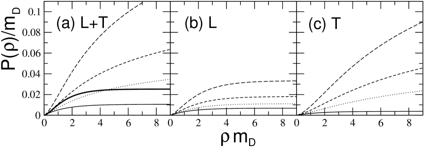
Figure 1: The function $P(\rho)$ (9) in units of the Debye mass versus $\rho m_{D}$ for different values of the ratio $\tau=T/m_{D}$. (a) shows the total $L+T$ contribution, (b) and (c) show $L$ and $T$ contributions, respectively. The curves correspond to: $\tau=0$ (solid line), $\tau=0.5$ (dotted line), $\tau=1$ (short dashes), $\tau=2$ (long dashes). The thick solid line in panel (a) shows prediction of the static model obtained with the dipole cross section (11).

The quadratic approximation $P(\rho)\propto\rho^{2}$ in the LCPI approach is equivalent to the Fokker-Planck approximation in Migdal’s approach [21]. It is not very accurate but reasonable for bremsstrahlung in ordinary materials. In this case the dominating $\rho$-scale is $\sim 1/m_{e}x$, and the spectrum is controlled by behavior of $P(\rho)$ at the scale $\sim 1/m_{e}$ which is much smaller than the screening radius $\sim 1/\alpha m_{e}Z^{1/3}$ (here $Z$ is the atomic number). In the case of the relativistic electron gas the situation is quite different. Now, in the dominating $\rho$-region, the argument of $P(\rho)$ is $\sim(0.1\div 2)/m_{D}$. In this region $P(\rho)$ is essentially non-quadratic. It is well seen from Fig. 1a, in which we plot the results of numerical calculations of $P(\rho)$ for several values of the ratio $T/m_{D}$. The results are presented in a dimensionless form. For comparison in Fig. 1a we also show the predictions of the static approximation at $T=0$ (when $m_{D}=\mu\sqrt{4\alpha/\pi}$) obtained with the dipole cross section (11). One can see that at $\rho\sim(0.1\div 2)/m_{D}$ the function $P(\rho)$ is almost linear in $\rho$.

To demonstrate the relative effect of the longitudinal and transverse modes in Figs. 1b,c we show separately the contributions related to $\Pi_{L}$ and $\Pi_{T}$. One sees that at $\rho\mathrel{\hbox to0.0pt{\lower 4.0pt\hbox{\hskip 1.0pt$\sim$}\hss}\raise 1.0pt\hbox{$<$}}1/m_{D}$ the L and T contributions are close to each other. However, at $\rho\mathrel{\hbox to0.0pt{\lower 4.0pt\hbox{\hskip 1.0pt$\sim$}\hss}\raise 1.0pt\hbox{$>$}}2/m_{D}$ the longitudinal part flattens, while the transverse magnetic one continues to grow (for $T/m_{D}$ not very close to zero). This growth of the transverse part is a consequence of the well known absence of the static magnetic screening in the electron plasma. Note, however, that from the point of view of the photon emission the growth of the magnetic contribution with $\rho$ is not important since the photon spectrum is dominated by $\rho\mathrel{\hbox to0.0pt{\lower 4.0pt\hbox{\hskip 1.0pt$\sim$}\hss}\raise 1.0pt\hbox{$<$}}1/\epsilon\sim 1/m_{D}$.

The growth of $P(\rho)$ with temperature is due to the presence of the Bose-Einstein factor in the function $D$ (A.1). From Fig. 1a one can see that the prediction of the HDL approximation at $T\ll m_{D}$, similarly to the static model, flatten at $\rho\mathrel{\hbox to0.0pt{\lower 4.0pt\hbox{\hskip 1.0pt$\sim$}\hss}\raise 1.0pt\hbox{$>$}}2/m_{D}$. However, the static model exceeds the HDL prediction by a factor $\sim 2.5$. The fact that at $T=0$ the static approximation overestimates $P(\rho)$ is quite natural, since the Pauli-blocking effects reduce the effective number of the scatterers. Note, however, that it would be incorrect to interpret the growth of $P(\rho)$ with temperature as an artifact associated only with the decrease of the Pauli-blocking at high temperatures. The function $P(\rho)$ in the HDL approximation accumulate all the collective effects in the soft modes of electromagnetic field in the electron plasma at the momentum scale $\sim m_{D}\ll\mu$. In particular, it accounts for the temperature dependence of the density of the plasmon excitations. Note that, physically, the appearance of $P(\rho)$ is due to Landau damping of the longitudinal and transverse modes.

It is worth noting that the collective effects cannot be accounted for consistently in the naive modification of the photon propagator in the amplitude of elastic $e^{-}e^{-}\to e^{-}e^{-}$ scattering as was assumed in [13]. One of the consequence of the inadequacy of this prescription is a strong overestimate of the magnetic contribution in [13]. It is connected with the $1/\theta^{4}$ ($\theta$ is the scattering angle) behavior of the magnetic contribution to elastic $e^{-}e^{-}\to e^{-}e^{-}$ cross section. To perform the $\theta$-integration the authors of [13] introduced some minimal momentum transfer. In contrast to [13] the magnetic contribution to the function $D(\mbox{{\bf q}}_{\perp})$ is $\propto 1/\mbox{{\bf q}}^{2}_{\perp}$ at $\mbox{{\bf q}}_{\perp}\to 0$, and the $\mbox{{\bf q}}_{\perp}$-integration in the formula for $P(\rho)$ (9) converges at small $\mbox{{\bf q}}_{\perp}$. This change in the small angle behavior of the magnetic contribution in the prescription of [13] and in our approach is connected with the dynamical magnetic screening which was not consistently accounted for in [13]. In principle, physically, it is evident that the concept of the elastic $e^{-}e^{-}\to e^{-}e^{-}$ amplitude itself is ill-defined for the momentum transfer $\mathrel{\hbox to0.0pt{\lower 4.0pt\hbox{\hskip 1.0pt$\sim$}\hss}\raise 1.0pt\hbox{$<$}}m_{D}$, where the collective effects come into play.

Note that in terms of $P(\rho)$ the transverse momentum broadening distribution of an electron propagating a distance $L$ through the electron gas can be written as [29]

$$I(\mbox{{\bf q}}_{\perp})=\frac{1}{(2\pi)^{2}}\int d\mbox{{\boldmath$\rho$}}\exp{[i\mbox{{\bf q}}_{\perp}\mbox{{\boldmath$\rho$}}-LP(\rho)]}\,.$$ (12)

This formula looks like the prediction of the eikonal approximation which neglects the variation of the electron tranverse coordinate. However, the path integral calculations [29] show that it is valid beyond the eikonal approximation as well.

Let us turn to calculation of the spectrum with the help of (5). Treating $v_{f}$ as a perturbation one can write

$${\cal K}(\xi_{2},\mbox{{\boldmath$\rho$}}_{2}|\xi_{1},\mbox{{\boldmath$\rho$}}_{1})={\cal K}_{m}(\xi_{2},\mbox{{\boldmath$\rho$}}_{2}|\xi_{1},\mbox{{\boldmath$\rho$}}_{1})-i\int d\xi d\mbox{{\boldmath$\rho$}}{\cal K}_{m}(\xi_{2},\mbox{{\boldmath$\rho$}}_{2}|\xi,\mbox{{\boldmath$\rho$}})v_{f}(\mbox{{\boldmath$\rho$}}){\cal K}_{m}(\xi,\mbox{{\boldmath$\rho$}}|\xi_{1},\mbox{{\boldmath$\rho$}}_{1})+\dots\,\,,$$ (13)

where ${\cal K}_{m}$ is the Green’s function for $v_{f}=0$. Then (5) can be written as

$$\frac{dP}{dxdL}=\frac{dP_{m}}{dxdL}+\frac{dP_{f}}{dxdL}\,.$$ (14)

Here the first term on the right-hand side comes from the ${\cal K}_{m}-{\cal K}_{v}$ in (5) after representing ${\cal K}$ in the form (13). It corresponds to the photon emission in a smooth mean field. The second term comes from the series in $v_{f}$ in (13). This term can be viewed as the radiation rate due to electron multiple scattering in the fluctuating field in the presence of a smooth external field.

The analytical expression for the Green’s function for the Hamiltonian with a constant force is known (see, for example [33]). In our case the ${\cal K}_{m}$ can be written as

$${\cal K}_{m}(\xi_{2},\mbox{{\boldmath$\rho$}}_{2}|\xi_{1},\mbox{{\boldmath$\rho$}}_{1})\!=\!\frac{M}{2\pi i\xi}\exp\left\{i\left[\frac{M(\mbox{{\boldmath$\rho$}}_{2}-\mbox{{\boldmath$\rho$}}_{1})^{2}}{2\xi}-\frac{x\xi\mbox{{\bf f}}\cdot(\mbox{{\boldmath$\rho$}}_{2}+\mbox{{\boldmath$\rho$}}_{1})}{2}-\frac{x^{2}\mbox{{\bf f}}^{2}\xi^{3}}{24M}-\frac{\xi}{L_{0}}\right]\right\}$$ (15)

with $\xi=\xi_{2}-\xi_{1}$. With this expression from (5) after simple calculations one can obtain a spectrum similar to the well known quasiclassical synchrotron spectrum [34] which can be written in terms of the Airy function $\mbox{Ai}(z)=\frac{1}{\pi}\sqrt{\frac{z}{3}}K_{1/3}(2z^{3/2}/3)$ (here $K_{1/3}$ is the Bessel function). In the case of interest, for a nonzero photon quasiparticle mass it reads [27]

$$\frac{dP_{m}}{dxdL}=\frac{a}{\kappa}\mbox{Ai}^{{}^{\prime}}(\kappa)+b\int_{\kappa}^{\infty}dy\mbox{Ai}(y)\,,$$ (16)

where $a=-{2\epsilon^{2}g_{1}}/{M}$, $b=Mg_{2}-{\epsilon^{2}g_{1}}/{M}$, $\kappa=\epsilon^{2}/(M^{2}x^{2}\mbox{{\bf f}}^{2})^{1/3}$. Inspecting the longitudinal integrals for the photon radiation in an external field one can find that the effective photon formation length for the mean field mechanism is given by $\bar{L}_{m}\sim\mbox{min}(L_{0},L_{m})$, where $L_{m}=(24M/x^{2}\mbox{{\bf f}}^{2})^{1/3}$ [27]. A similar estimate can be obtained from the criterion of separation of the photon and electron wave packets. Note that the analytical expression for the Green’s function for the oscillator with a constant force is known as well (see [33]). Making use of this Green’s function one can obtain for $P(\rho)\propto\rho^{2}$ the radiation rate in the form given in [35], where Migdal’s approach within the Fokker-Planck approximation was generalized to the case with an external field. The formulas of [35] were used in [15]. However, as already noted the approximation $P(\rho)\propto\rho^{2}$ is clearly not adequate for the electrosphere.

Let us discuss now the fluctuation component ${dP_{f}}/{dxdL}$. We represent it in the form

$$\frac{dP_{f}}{dxdL}=\frac{dP_{f}^{BH}}{dx}+\frac{dP_{f}^{LPM}}{dx}\,,$$ (17)

where the first term on the right-hand side corresponds to the leading order in expansion in $v_{f}$ in (13), and the second one to the sum of the higher order terms. The $dP_{f}^{BH}/dxdL$ is the analog of the Bethe-Heitler spectrum in ordinary materials, while the $dP_{f}^{LPM}/dxdL$ describes the LPM correction. For the Bethe-Heitler term one can obtain from (5), (13)

$$\frac{dP_{f}^{BH}}{dx}=2\int d\mbox{{\boldmath$\rho$}}\,W(x,\mbox{{\boldmath$\rho$}},\mbox{{\bf f}})P(\rho x)\,,$$ (18)

$$W(x,\mbox{{\boldmath$\rho$}},\mbox{{\bf f}})=-\mbox{Re}\,\,\hat{g}(x)\Phi(x,\mbox{{\boldmath$\rho$}},\mbox{{\boldmath$\rho$}}_{1},\mbox{{\bf f}})\Phi(x,\mbox{{\boldmath$\rho$}},\mbox{{\boldmath$\rho$}}_{2},\mbox{{\bf f}})\Big{|}_{\mbox{{\boldmath$\rho$}}_{1}=\mbox{{\boldmath$\rho$}}_{2}=0}\,,$$ (19)

$$\Phi(x,\mbox{{\boldmath$\rho$}},\mbox{{\boldmath$\rho$}}^{\prime},\mbox{{\bf f}})=\int_{-\infty}^{0}d\xi{\cal K}_{m}(\mbox{{\boldmath$\rho$}},0|\mbox{{\boldmath$\rho$}}^{\prime},\xi)\,.$$ (20)

Note that for a nonzero f the function $W$ cannot be viewed as a probability density for the $|\gamma e\rangle$ Fock component of the physical photon (it is even not positively defined). This is connected with the fact that in an external field the $|\gamma e\rangle$ Fock component is not stable, and decays through the tunnel transition into free photon and electron. The analog of the representation for the LPM correction derived in [19] for nonzero mean field reads

$$\frac{dP_{f}^{LPM}}{dx}=2\mbox{Re}\,\hat{g}(x)\int\limits_{0}^{\infty}d\xi\int d\mbox{{\boldmath$\rho$}}\,\Phi(x,\mbox{{\boldmath$\rho$}},\mbox{{\boldmath$\rho$}}_{2},\mbox{{\bf f}})P(\rho x)\tilde{\Phi}(x,\mbox{{\boldmath$\rho$}},\mbox{{\boldmath$\rho$}}_{1},\mbox{{\bf f}},\xi)\Big{|}_{\mbox{{\boldmath$\rho$}}_{1}=\mbox{{\boldmath$\rho$}}_{2}=0}\,,$$ (21)

where the function $\tilde{\Phi}(x,\mbox{{\boldmath$\rho$}},\mbox{{\boldmath$\rho$}}_{1},\mbox{{\bf f}},\xi)$ is the solution of the two-dimensional Schrödinger equation with the Hamiltonian (7). The boundary condition for $\tilde{\Phi}(x,\mbox{{\boldmath$\rho$}},\mbox{{\boldmath$\rho$}}_{1},\mbox{{\bf f}},\xi)$ is $\tilde{\Phi}(x,\mbox{{\boldmath$\rho$}},\mbox{{\boldmath$\rho$}}_{1},\mbox{{\bf f}},0)=\Phi(x,\mbox{{\boldmath$\rho$}},\mbox{{\boldmath$\rho$}}_{1},\mbox{{\bf f}})P(\rho x)\,.$

In the case of zero f the function $W$ may be written as a density for the $|\gamma e\rangle$ Fock state

$$W(x,\mbox{{\boldmath$\rho$}})=\frac{1}{2}\sum\limits_{\{\lambda_{i}\}}|\Psi(x,\mbox{{\boldmath$\rho$}},\{\lambda_{i}\})|^{2}\,,$$ (22)

where $\Psi(x,\mbox{{\boldmath$\rho$}},\{\lambda_{i}\})$ is the light-cone wave function for the $e\to\gamma e^{\prime}$ transition, $\{\lambda_{i}\}=(\lambda_{e},\lambda_{e^{\prime}},\lambda_{\gamma})$ a set of helicities. Note that contrary to the case $\mbox{{\bf f}}\neq 0$ now, due to the azimuthal symmetry of the Hamiltonian, the light-cone wave functions have definite azimuthal quantum numbers. The LPM correction in this case also can be written in terms of the light-cone wave functions. The results is similar to that for ordinary materials [19, 21]

$$\frac{dP_{f}^{LPM}}{dx}=-\mbox{Re}\sum\limits_{\{\lambda_{i}\}}\int\limits_{0}^{\infty}d\xi\int d\mbox{{\boldmath$\rho$}}\,\Psi^{*}(x,\mbox{{\boldmath$\rho$}},\{\lambda_{i}\})P(\rho x)\tilde{\Phi}(x,\mbox{{\boldmath$\rho$}},\{\lambda_{i}\},\xi)\,.$$ (23)

The boundary condition for $\tilde{\Phi}(x,\mbox{{\boldmath$\rho$}},\{\lambda_{i}\},\xi)$ is now $\tilde{\Phi}(x,\mbox{{\boldmath$\rho$}},\{\lambda_{i}\},0)=\Psi(x,\mbox{{\boldmath$\rho$}},\{\lambda_{i}\})P(\rho x)\,.$ The light-cone wave functions appear in the formulas (22), (23) from the $\xi$-integrals in (5) and (13) of the Green’s function ${\cal K}_{m}$ and action of the vertex operator written in terms of the helicity projectors as was done in [17].

The formulas for the light-cone wave functions are given in the Appendix B. Making use of the formulas given there one can obtain for the probability distribution $W$ for the $e\to\gamma e^{\prime}$ transition at $\mbox{{\bf f}}=0$

$$W(x,\mbox{{\boldmath$\rho$}})=\frac{\alpha}{2\pi^{2}}\left\{\frac{[1+(1-x)^{2}]}{x}\epsilon^{2}K_{1}^{2}(\rho\epsilon)+x^{3}m_{e}^{2}K_{0}^{2}(\rho\epsilon)\right\}\,,$$ (24)

where $K_{0,1}$ are the Bessel functions. Due to exponential decrease of $K_{0,1}$ in (24) the dominating $\rho$ scale in the formula (18) for the fluctuation term is $\sim 1/\epsilon$.

For nonzero f the azimuthal symmetry is absent. This makes the problem considerably more complicated. In the present work we have first calculated the spectrum ${dP_{f}}/{dxdL}$ for $\mbox{{\bf f}}=0$. We observed that the LPM correction in (17) is negligible as compared to the Bethe-Heitler term. Also, the Bethe-Heitler term itself turns out to be much smaller than the mean field term $dP_{m}/dxdL$. It is clear that a nonzero f will make $dP_{f}/dxdL$ even smaller. For this reason an accurate calculation of the fluctuation term for nonzero f does not make much sense. We have taken into account the effect of the transverse force using qualitative arguments based on the estimates of the coherence lengths with and without tranverse force. The mean field should suppress the coherence length. The suppression of the radiation rate should be approximately the same [36]. Thus, the mean field suppression factor can be written as the ratio of the formation lengths with and without the mean field. The coherence length in the presence of the mean field is $\sim\bar{L}_{m}$. Without the mean field in the regime of weak LPM suppression the coherence length is given by $L_{0}$. So one has the mean field suppression factor $S_{m}\approx\bar{L}_{m}/L_{0}$. Note that due to reduction of the effective formation length the LPM effect should become even smaller for a nonzero mean field.

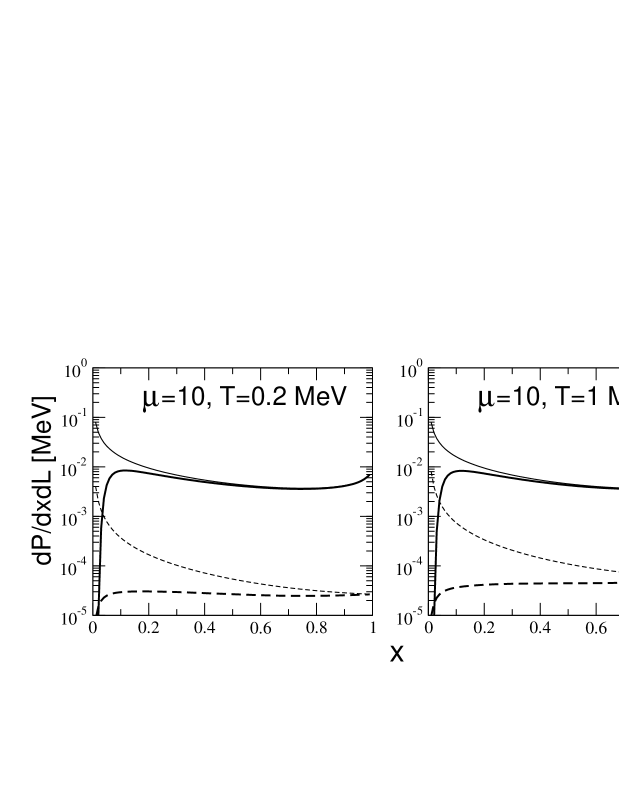
Figure 2: The contributions to the spectrum $dP/dxdL$ from the mean field mechanism (solid line) and the fluctuation mechanism (dashes) for $\mu=10$ MeV at $T=0.2$ and $T=1$ MeV. The thick curves are for nonzero photon mass, and the thin ones are for massless photon. The contribution of the fluctuation mechanism is calculated using the Bethe-Heitler term with the distribution (24).

To illustrate the relative contributions of the mean field and fluctuation mechanisms to $dP/dxdL$ we plot them in Fig. 2 for $\mu=10$ MeV and $T=0.2$ and $T=1$ MeV. The mean field part shown in Fig. 2 corresponds to the spectrum averaged over all directions of the electron momentum. The fluctuation contribution has been calculated without the mean field suppression factor. Note that we perform calculations with the $k$-dependent photon quasiparticle mass extracted from the relation $m^{2}_{\gamma}=\Pi_{T}(\sqrt{k^{2}+m^{2}_{\gamma}},k)$ . This gives $m_{\gamma}$ rising from $m_{D}/\sqrt{3}$ at $k\ll m_{D}$ to $m_{D}/\sqrt{2}$ at $k\gg m_{D}$ with the Debye mass $m_{D}^{2}=\frac{4\alpha}{\pi}(\mu^{2}+\pi^{2}T^{2}/3)$. From Fig. 2 one sees that the fluctuation contribution is suppressed by a factor $\sim 10^{-2}$. To illustrate the role of the finite photon quasiparticle mass we presented in Fig. 2 the results for zero $m_{\gamma}$ as well (thin curves). It is seen that the photon mass suppression (called usually the Ter-Mikaelian effect) is very strong at small $x$. The effect is especially dramatic for the fluctuation part where the well known $1/x$ form of the spectrum is changed into $\propto x$. This effect was ignored in the analyses [14, 15] where the massless formulas have been used. The results shown in Fig. 2 indicate clearly that the massless approximation is inadequate.

As previously mentioned, our calculations show that for the fluctuation mechanism the LPM suppression is negligible. This is in a contradiction with the analysis [13] where the authors find a very strong LPM suppression (about $\sim 1/300$ at the photon momentum $k=0.5$ MeV for electron energy $10$ MeV). For calculation of the LPM suppression the authors of [13] have used Migdal’s formulas with zero photon mass putting there $Z=1$ . However, one can easily show that Migdal’s formulas become inadequate for the electrosphere. We explain this in the language of the LCPI approach. Migdal’s approach [24] corresponds in the LCPI formalism to quadratic parametrization $P(\rho)\approx nC\rho^{2}/2$. As described above, this approximation is not accurate for electrosphere, but nevertheless it is suitable for our qualitative analysis. In the quadratic approximation the Hamiltonian (7) takes the oscillator form with $\Omega=\sqrt{-inCx^{2}/M(x)}$. The LPM suppression factor, $S_{LPM}$, can be written in terms of the dimensionless parameter $\eta=|\Omega|L_{0}$ [18, 21]. The LPM suppression becomes strong at $\eta\gg 1$. In this limit $S_{LPM}\approx 3/\eta\sqrt{2}$ [18]. The LPM effect is negligible for $\eta\ll 1$ when $S_{LPM}(\eta)\approx 1-16\eta^{4}/21$ [18], Note that even at $\eta\sim 1$ the LPM suppression is relatively small since $S_{LPM}(1)\approx 0.86$. A very strong suppression obtained in [13] is mostly due to the neglect of the photon mass. The finite photon mass reduces strongly the $L_{0}$ and correspondingly the parameter $\eta$ (about a factor $\sim 400$ for $k=0.5$ and $p\sim 10$ MeV). Also, for the electrosphere there is no the well known large Coulomb logarithm $\ln(1/\alpha)\sim 5$ (which comes from the logarithm in the dipole cross section [20]) in the $|\Omega|$, which is present in Migdal’s formulas derived for ordinary materials. Both these effects reduce drastically the value of $\eta$ for the electrosphere as compared to that in Migdal’s approach. As a result, the LPM suppression in the electrosphere turns out to be negligible.

4 Numerical results and discussion

In this section we present the numerical results for the emissitivity and radiated energy flux. The results were obtained with some modification of the spectrum $dP/dxdL$ in the noncollinear region. As we mentioned earlier, the collinear approximation we use becomes invalid for very soft photons with $k\mathrel{\hbox to0.0pt{\lower 4.0pt\hbox{\hskip 1.0pt$\sim$}\hss}\raise 1.0pt\hbox{$<$}}m_{\gamma}$. In this region the formalisms [16, 17, 18] do not apply. In particular, the LCPI approach [18], which assumes that the transverse momentum integration comes up to infinity, should overestimate the photon spectrum at $k\mathrel{\hbox to0.0pt{\lower 4.0pt\hbox{\hskip 1.0pt$\sim$}\hss}\raise 1.0pt\hbox{$<$}}m_{\gamma}$. To take into account this effect (at least, qualitatively) in calculating the radiated energy flux we multiplied $dP/dxdL$ by the kinematical suppression factor $S_{kin}(k)=1-\exp(-k^{2}/m_{\gamma}^{2})$. This factor does not give a big effect. It suppresses the radiated energy by $\sim 10-15$% at $T\sim 0.1\div 0.2$ MeV and $\sim 1-2$% at $T\sim 1$ MeV. This says that the errors from the noncollinear configurations are small.

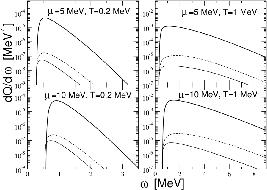
Figure 3: The emissitivity versus the photon energy $\omega$ for $\mu=5$ and $\mu=10$ MeV at $T=0.2$ and $T=1$ MeV. The thick solid line shows the mean field bremsstrahlung. The contribution of the fluctuation mechanism is shown without (dashes) and with (thin solid line) the mean field suppression.

In Fig. 3 we show the emissitivity for $\mu=5$ and $\mu=10$ MeV evaluated for $T=0.2$ and $T=1$ MeV as a function of $\omega$. One sees that the contribution of the mean field emission (thick solid line) exceeds the fluctuation emission without mean field suppression (dashes) by a factor $\sim 10^{2}$. The mean field suppression gives additional reduction of the fluctuation contribution (thin solid line) by a factor $\sim 3-4$. Note that in our quasiclassical approximation at a given $\mu$ there is no photon emission at $\omega<\omega_{p}^{e}$. For this reason the differential emissitivity shown in Fig. 3 vanishes abruptly at $\omega=\omega_{p}^{e}=m_{\gamma}(k=0)$. From Fig. 3 one can see that, despite the Pauli-blocking suppression, even at $T=0.2$ MeV the contribution of energetic photons with energy about several units of $\omega_{p}^{e}$ is important. This demonstrates that the restriction on the photon energy $\omega<\sqrt{\omega_{p}^{e\,2}+m_{e}^{2}}$ imposed by the authors of [13] is clearly inadequate.

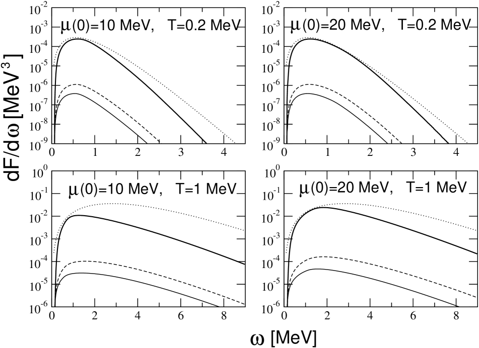
Figure 4: The differential radiated energy flux from the electrosphere for the mean field bremsstrahlung (thick solid line) and for the Bethe-Heitler bremsstrahlung with (thin solid line) and without (dashes) the mean field suppression. The dotted curves show the black body spectrum.

In Fig. 4 we plot the differential radiated energy flux $dF/d\omega$ for $\mu(0)=10$ and $\mu(0)=20$ MeV obtained for $T=0.2$ and $T=1$ MeV. For the fluctuation contribution we show the results with and without the mean field suppression factor $S_{m}$. For comparison the black body spectrum is also shown. The mean Coulomb field of the electrosphere reduces the fluctuation term by a factor $\sim 3-4$. From Fig. 3, 4 one can see that the relative contribution of the fluctuation mechanism is very small compared to the mean field emission. Thus, in some sense we have a situation similar to that for photon radiation from an atom with large $Z$. Note that the form of the spectrum for the mean field mechanism is qualitatively similar to that for the black body radiation.

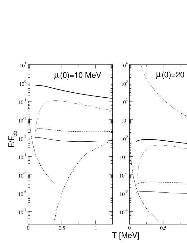
Figure 5: The total radiated energy flux (scaled to the black body radiation) from the electrosphere for the mean field bremsstrahlung (thick solid line) and for the Bethe-Heitler bremsstrahlung with (thin solid line) and without (short dashes) the mean field suppression. The contribution from the the tunnel $e^{+}e^{-}$ creation [4, 10] evaluated using (25) is also shown (dotted line). The long dashes show the results for $e^{-}+e^{-}\to e^{-}+e^{-}+\gamma$ process obtained in [13]. The dot-dashed line show the results for the same process of [14]. The dot-dot-dashed line shows the bremsstrahlung contribution with inclusion of the mean Coulomb field of [15].

In Fig. 5 we show the total energy flux $F=\int_{0}^{\infty}d\omega{dF}/{d\omega}$ scaled to the black body radiation as a function of temperature. For comparison we also plot the predictions for bremsstrahlung obtained in [13, 14, 15]. We also show there the energy flux from the $e^{+}e^{-}$ pair production [4, 10]. We define it as

$$F_{\pm}=\int_{0}^{h_{max}}dhQ_{\pm}(h)\approx\sqrt{\frac{3\pi}{2\alpha}}\int_{\mu_{min}}^{\mu(0)}\frac{d\mu}{\mu^{2}}Q_{\pm}(h(\mu))\,.$$ (25)

Here $Q_{\pm}$ is the energy flux from $e^{+}e^{-}$ pairs per unit time and volume. We write it as in [4, 10] $Q_{\pm}=E_{e^{+}e^{-}}dN_{e^{+}e^{-}}/dtdV$, where $E_{e^{+}e^{-}}\approx 2(m_{e}+T)$ is the typical energy of $e^{+}e^{-}$ pairs, and $dN_{e^{+}e^{-}}/dtdV$ the rate of $e^{+}e^{-}$ pair production per unit time and volume given by

$$\frac{dN_{e^{+}e^{-}}}{dtdV}\approx\frac{3T^{3}\mu}{2\pi^{3}}\sqrt{\frac{\alpha}{\pi}}\exp{\left(-\frac{2m_{e}}{T}\right)}J(\xi)$$ (26)

with $\xi=\frac{2\mu}{T}\sqrt{\frac{\alpha}{\pi}}$, and the function $J$ is defined as in [10]

$$J(x)=\frac{x^{3}\ln{(1+2/x)}}{3(1+0.074x)^{3}}+\frac{\pi^{5}x^{4}}{6(13.9+x)^{4}}\,.$$

From Fig. 5 one sees that in the region $T\sim 0.1\div 1$ MeV the mean field photon emission exceeds considerably both the fluctuation bremsstrahlung and the energy flux from $e^{+}e^{-}$ pair production.

Figs. 4, 5 demonstrate that the energy flux from the mean field photon emission may be of the same order of magnitude as the black body radiation. It says that the approximation of optically thin electrosphere is not very good, and the photon absorption and stimulated emission may be important. However, since the radiation rate we obtained does not exceed the black body limit, they can not modify strongly our results. Note that the authors of [15] obtained for $T\mathrel{\hbox to0.0pt{\lower 4.0pt\hbox{\hskip 1.0pt$\sim$}\hss}\raise 1.0pt\hbox{$<$}}1$ MeV the energy flux considerably exceeding the black body limit. This can be seen from Fig. 5, where the results of [15] at $\mu(0)=20$ MeV are shown. The authors of [15] claim that the electrosphere may radiate stronger than a black body. This statement is obviously incorrect. The violation of the black body limit in [15] is just a signal that the thin medium approximation becomes inadequate at high emissitivity. As far as a very large emissitivity obtained in [15] is concerned, as we already mentioned, it may be due to incorrect description of the Pauli-blocking and neglect of the photon mass.

As we mentioned earlier, our assumption that the photon emission is a local process is valid if $l_{f}\sim\bar{L}_{m}\ll L_{el}$, where $L_{el}$ is the typical scale of variation of the potential $v_{m}$ along the electron trajectory. For the chemical potential (1) it can be defined as $L_{el}\sim H\mu(0)/\mu(h)\cos{\theta}$, where $\theta$ is the angle between the electron momentum and the star surface normal. Evidently, the contribution of the configurations with $\bar{L}_{m}\mathrel{\hbox to0.0pt{\lower 4.0pt\hbox{\hskip 1.0pt$\sim$}\hss}\raise 1.0pt\hbox{$>$}}L_{el}$ into the photon spectrum will be suppressed by the finite-size suppression factor $S_{fs}\sim\mbox{min}(L_{el},\bar{L}_{m})/\bar{L}_{m}$. We have checked numerically that this suppression factor gives a negligible effect. This justifies the local approximation.

According to the simulation of the thermal evolution of young quark stars performed in [25] the temperature at the star’s surface becomes $\sim 0.2$ MeV at $t\sim 1$ s. However, in the analysis [25] the mean field bremsstrahlung was not taken into account. In the light of our results one can expect that the cooling of the bare quark star’s surface should go somewhat faster than predicted in [25]. It is worth noting that in the initial stage of the quark star evolution the mean field photon emission can only modify the temperature near the star surface. The evolution of the star core temperature is driven by the neutrino emission [25] since for an extended period of time the neutrino luminosity is much larger than the photon (and $e^{+}e^{-}$) luminosity [25]. Higher luminosity due to the mean field bremsstrahlung increases the possibility for detecting bare quark stars. From the point of view of the light curves at $t\mathrel{\hbox to0.0pt{\lower 4.0pt\hbox{\hskip 1.0pt$\sim$}\hss}\raise 1.0pt\hbox{$>$}}1$ s it would be interesting to investigate the mean field bremsstrahlung for $T\mathrel{\hbox to0.0pt{\lower 4.0pt\hbox{\hskip 1.0pt$\sim$}\hss}\raise 1.0pt\hbox{$<$}}0.1$ MeV as well. However, at such temperatures the photon emission from the nonrelativistic region of the electrosphere may be important, where our formulas become inapplicable. As far as the contribution of the relativistic region $\mu\gg m_{e}$ is concerned. Extrapolation of the curves shown in Fig. 5 to $T\mathrel{\hbox to0.0pt{\lower 4.0pt\hbox{\hskip 1.0pt$\sim$}\hss}\raise 1.0pt\hbox{$<$}}0.1$ MeV allows one to expect that the mean field emission will dominate the energy flux at lower temperatures as well.

A remark is in order here on the photon distribution seen by a distant observer. For obtained values of the energy flux the radiation cannot stream outward freely. The point is that near the star surface the thermalization time in the comoving frame for the $e^{+}e^{-}\gamma$ wind is negligibly small as compared to the star radius. This follows from estimates of the mean free path, $\lambda$, related to $\gamma+e^{\pm}\rightarrow\gamma+e^{\pm}$ and $\gamma+\gamma\leftrightarrow e^{+}+e^{-}$ processes. The qualitative calculations give $\lambda\sim 10^{-3}$cm at $T\sim 0.1$ MeV and $\lambda\sim 10^{-6}$cm at $T\sim 1$ MeV. For this reason the $e^{+}e^{-}\gamma$ wind can be described as a hydrodynamical flow. The hydrodynamical description is valid up the the freezeout surface, beyond which the radiation streams outward almost freely. For an observer at large distance from the star the photon spectrum is close to the black body one with a temperature $T_{ext}=T_{fr}\Gamma_{fr}$, where $T_{fr}$ is the wind temperature and $\Gamma_{fr}$ the bulk Lorentz factor of the wind at the freezeout level [38, 39]. One can show that for a relativistic wind $T_{fr}\Gamma_{fr}\approx T_{i}\Gamma_{i}$ [38, 39], where $T_{i}$ is the wind temperature after its thermalization and $\Gamma_{i}$ the bulk Lorentz factor of the wind near the star surface. For $T\sim 0.1$ MeV the electron fraction in the $e^{+}e^{-}\gamma$ wind after thermalization is small. Simple qualitative calculations give in this case $T_{i}\Gamma_{i}\approx T(3\kappa\Gamma_{i}^{2}/16)^{1/4}$, where $\kappa=(F+F_{\pm})/F_{bb}$. As a plausible estimates one can take $\Gamma_{i}^{2}\sim 3$ and $\kappa\sim 1$. Then one obtains $T_{ext}\sim 0.85T$. For $T\sim 1$ MeV the electron fraction in the wind after thermalization becomes close to that for relativistic plasma. In this case $T_{i}\Gamma_{i}\approx T(3\kappa\Gamma_{i}^{2}/44)^{1/4}$. Taking $\kappa\sim 0.4$ one obtains $T_{ext}\sim 0.5T$. Note that in both the cases beyond the freezeout surface the fraction of $e^{\pm}$ pairs in the wind is negligibly small [39].

Note that our calculations probably do not apply to quark stars in the color flavor locked (CFL) superconducting phase. Previously it was suggested [40] that, despite the absence of electrons in the bulk SQM in the CFL phase, the electrosphere may exist due to the surface quark charge [41]. However, the recent analysis [42] gives evidence in favor of absence of such a surface charge. But for the CFL phase may exist a significant photon emission from the SQM itself due to the photon-gluon mixing [43]. The results of [43] show that this radiation is comparable to the black body limit. Since we also obtain the radiation rate comparable to the black body radiation it may be difficult to distinguish a bare quark star in the CFL phase from that in normal (or 2SC) phase.

5 Conclusion

In summary, we have evaluated the photon emission from the electrosphere of a bare quark star (in normal or 2SC phase). The analysis is based on the LCPI reformulation [17] of the AMY formalism [16] to the photon emission from relativistic plasmas. The developed approach, contrary to the previous qualitative studies [13, 14, 15], allows, for the first time, to give a robust treatment of the Pauli-blocking effects in the photon bremsstrahlung. We demonstrate that for the temperatures $T\sim 0.1\div 1$ MeV the dominating contribution to the photon emission is due to bending of electron trajectories in the mean electric field of the electrosphere. The energy flux from the mean field photon emission is of order of the black body limit. Our results show that the contribution of the Bethe-Heitler bremsstrahlung due to electron-electron interaction is negligible as compared to the mean field photon emission. In contrast with [13] we demonstrate that the LPM suppression is negligible.

The energy flux related to the mean field bremsstrahlung turns out to be larger than that from the tunnel $e^{+}e^{-}$ pair creation [4, 10] as well. In the light of these results the situation with distinguishing bare quark stars made of the SQM in normal (or 2SC) phase from neutron stars may be more optimistic than in the scenario with the tunnel $e^{+}e^{-}$ creation discussed in [25].

Acknowledgements

I would like to thank J.F. Caron for providing the file for the radiated energy flux obtained in [14]. I am also grateful to T. Harko and D. Page for communication. This work is supported in part by the grant SS-6501.2010.2.

Appendix A. Calculation of the function $D(\mbox{{\bf q}}_{\perp})$

In this appendix, we discuss the calculation of the function $D(\mbox{{\bf q}}_{\perp})$. To evaluate this function one needs to know the correlator $D^{\mu\nu}$. In momentum representation one can obtain

$$D^{\mu\nu}(q)=-2[1+n_{B}(q_{0})]\mbox{Im}D^{\mu\nu}_{r}(q)\,,$$

where $n_{B}=[\exp(q_{0}/T)-1]^{-1}$ is the Bose-Einstein factor, and $D^{\mu\nu}_{r}(q)$ retarded Green’s function. As was already noted the function $P(\rho)$ is gauge invariant, and one can use $D^{\mu\nu}_{r}$ in any gauge. Expressing the retarded propagator in the Coulomb gauge in terms terms of longitudinal and transverse photon self-energies one can obtain

$$D(\mbox{{\bf q}}_{\perp})=-\frac{1}{\pi}\int\limits_{-\infty}^{\infty}dq_{0}\frac{\exp(q_{0}/T)}{\exp(q_{0}/T)-1}\left\{\frac{{\rm Im}\Pi_{L}(q_{0},\mbox{{\bf q}})}{[\mbox{{\bf q}}^{2}-{\rm Re}\Pi_{L}(q_{0},\mbox{{\bf q}})]^{2}+({\rm Im}\Pi_{L}(q_{0},\mbox{{\bf q}}))^{2}}\right.$$

$$\left.+\left.\frac{\mbox{{\bf q}}_{\perp}^{2}}{\mbox{{\bf q}}^{2}}\dot{\frac{{\rm Im}\Pi_{T}(q_{0},\mbox{{\bf q}})}{[\mbox{{\bf q}}_{\perp}^{2}+{\rm Re}\Pi_{T}(q_{0},\mbox{{\bf q}})]^{2}+({\rm Im}\Pi_{T}(q_{0},\mbox{{\bf q}}))^{2}}}\right\}\right|_{q_{z}=q_{0}}\,\,.$$ (A.1)

In numerical calculations we use for $\Pi_{L,T}$ the HDL expressions [30, 31]

$$\Pi_{L}(q_{0},\mbox{{\bf q}})=m_{D}^{2}\left[\frac{q_{0}}{2q}\ln\left(\frac{q_{0}+q}{q_{0}-q}\right)-1\right]\,,$$ (A.2)

$$\Pi_{T}(q_{0},\mbox{{\bf q}})=\frac{m_{D}^{2}}{2}\left[\frac{q_{0}^{2}}{q^{2}}+\frac{(q^{2}-q_{0}^{2})q_{0}}{2q^{3}}\ln\left(\frac{q_{0}+q}{q_{0}-q}\right)-1\right]$$ (A.3)

with the Debye mass $m_{D}^{2}=\frac{4\alpha}{\pi}(\mu^{2}+\pi^{2}T^{2}/3)$.

Appendix B. Formulas for the light-cone wave functions

For zero f the light-cone wave functions have definite orbital quantum number $m$. As was mentioned the light-cone wave functions appear from the longitudinal integrals of the Green’s function. For $\mbox{{\bf f}}=0$ it is the free Green’s function given by

$${\cal K}_{v}(\xi_{2},\mbox{{\boldmath$\rho$}}_{2}|\xi_{1},\mbox{{\boldmath$\rho$}}_{1})\!=\!\frac{M}{2\pi i\xi}\exp\left\{i\left[\frac{M(\mbox{{\boldmath$\rho$}}_{2}-\mbox{{\boldmath$\rho$}}_{1})^{2}}{2\xi}-\frac{\xi\epsilon^{2}}{2M}\right]\right\}$$ (B.1)

with $\xi=\xi_{2}-\xi_{1}$. The $\xi$-integration can be performed with the help of the relation

$$\int_{-\infty}^{0}d\xi{\cal K}_{v}(\mbox{{\boldmath$\rho$}}_{2},0|\mbox{{\boldmath$\rho$}}_{1},\xi)=-\frac{iM}{\pi}K_{0}(|\mbox{{\boldmath$\rho$}}_{2}-\mbox{{\boldmath$\rho$}}_{1}|\epsilon)\,,$$ (B.2)

where $K_{0}$ is the Bessel function. Then the light-cone wave functions can be written in terms of the Bessel functions $K_{0}$ and $K_{1}$. After representing the vertex operator (6) in terms of the helicity state projectors as in [17] one can obtain for $\lambda_{e^{\prime}}=\lambda_{e}$

$$\Psi(x,\mbox{{\boldmath$\rho$}},\lambda_{e},\lambda_{e^{\prime}},\lambda_{\gamma})=\frac{1}{2\pi}\sqrt{\frac{\alpha}{2x}}\left[\lambda_{\gamma}(2-x)+2\lambda_{e}x\right]\exp(-i\lambda_{\gamma}\varphi)\epsilon K_{1}(\rho\epsilon)\,,$$ (B.3)

where $\varphi$ is the azimuthal angle. For $\lambda_{e^{\prime}}=-\lambda_{e}$

$$\Psi(x,\mbox{{\boldmath$\rho$}},\lambda_{e},-\lambda_{e},2\lambda_{e})=\frac{-i}{2\pi}\sqrt{2\alpha x^{3}}m_{e}K_{0}(\rho\epsilon)\,.$$ (B.4)

References

- [1] E. Witten, Phys. Rev. D30, 272 (1984).
- [2] C. Alcock, E. Farhi, and A. Olinto, Astrophys. J. 310, 261 (1986).
- [3] P. Haensel, J.L. Zdunik, and R. Schaeffer, Astron. Astrophys. 160, 121 (1986).
- [4] V.V. Usov, Phys. Rev. Lett. 80, 230 (1998) [arXiv:astro-ph/9712304].
- [5] C. Kettner, F. Weber, and M.K. Weigel, Phys. Rev. D51, 1440 (1995).
- [6] T. Chmaj, P. Haensel, and W. Slominski, Nucl. Phys. B24, 40 (1991).
- [7] K.S. Cheng and T. Harko, Astrophys. J. 596, 451 (2003) [arXiv:astro-ph/0306482].
- [8] V.V. Usov, Phys. Rev. Lett. 87, 021101 (2001).
- [9] A.R. Zhitnitsky, JCAP 0310, 010 (2003) [arXiv:hep-ph/0202161]; M.M. Forbes and A.R. Zhitnitsky, JCAP 0801, 023 (2008) [arXiv:astro-ph/0611506]; M.M. Forbes and A.R. Zhitnitsky, Phys. Rev. D78, 083505 (2008).
- [10] V.V. Usov, Astrophys. J. 550, L179 (2001) [arXiv:astro-ph/0103361].
- [11] J. Schwinger, Phys. Rev. 82, 664 (1951).
- [12] A.G. Aksenov, M. Milgrom, and V.V. Usov, Astrophys. Space Sci. 308:613 (2007) [arXiv:astro-ph/0606613].
- [13] P. Jaikumar, C. Gale, D. Page, and M. Prakash, Phys. Rev. D70, 023004 (2004).
- [14] J. F. Caron and A.R. Zhitnitsky, Phys. Rev. D80, 123006 (2009).
- [15] T. Harko and K.S. Cheng, Astrophys. J. 622,1033 (2005) [arXiv:astro-ph/0412280].
- [16] P. Arnold, G.D. Moore and L.G. Yaffe, JHEP 0111, 057 (2001); JHEP 0112, 009 (2001); JHEP 0206, 030 (2002).
- [17] P. Aurenche and B.G. Zakharov, JETP Lett. 85, 149 (2007) [arXiv:hep-ph/0612343].
- [18] B.G. Zakharov, JETP Lett. 63, 952 (1996).
- [19] B.G. Zakharov, JETP Lett. 64, 781 (1996).
- [20] B.G. Zakharov, Phys. Atom. Nucl. 62, 1008 (1999) [arXiv:hep-ph/9805271].
- [21] B.G. Zakharov, Phys. Atom. Nucl. 61, 838 (1998) [arXiv:hep-ph/9807540].
- [22] B.G. Zakharov, Nucl. Phys. Proc. Suppl. 146, 151 (2005) [arXiv:hep-ph/0412177].
- [23] L.D. Landau and I.Ya. Pomeranchuk, Dokl. Akad. Nauk SSSR 92, 535, 735 (1953).
- [24] A.B. Migdal, Phys. Rev. 103, 1811 (1956).
- [25] D. Page and V.V. Usov, Phys. Rev. Lett. 89, 131101 (2002) [arXiv:astro-ph/0204275].
- [26] B.G. Zakharov, Phys. Lett. B690, 250 (2010) [arXiv:1003.5779 [hep-ph]].
- [27] B.G. Zakharov, JETP Lett. 88, 475 (2008) [arXiv:0809.0599 [hep-ph]].
- [28] L.D. Landau and E.M. Lifshitz, The classical theory of fields (Pergamon Press, 1975).
- [29] B.G. Zakharov, Sov. J. Nucl. Phys. 46, 92 (1987).
- [30] E. Braaten, Can. J. Phys. 71, 215 (1993) [arXiv:hep-ph/9303261].
- [31] E. Braaten and D. Segel, Phys. Rev. D48, 1478 (1993) [arXiv:hep-ph/9302213].
- [32] P. Aurenche, F. Gelis and H. Zaraket, JHEP 0205, 043 (2002) [arXiv:hep-ph/0204146].
- [33] R.P. Feynman and A. Hibbs, Quantum Mechanics and Path Integrals (McGraw Hill, New York, 1965).
- [34] V.N. Baier and V.M. Katkov, JETP 26, 854 (1968).
- [35] V.G. Baryshevskii and V.V. Tikhomirov, JETP 63, 116 (1986).
- [36] V.M. Galitsky and I.I. Gurevich, Il Nuovo Cim. 32, 396 (1964).
- [37] J. P. Blaizot and J.Y. Ollitrault, Phys. Rev. D48, 1390 (1993).
- [38] B. Paczynski, Astrophys. J. 308, L43 (1986).
- [39] O.M. Grimsrud and I. Wasserman, arXiv:astro-ph/9805138.
- [40] V.V. Usov, Phys. Rev. D70 067301 (2004).
- [41] J. Madsen, Phys. Rev. Lett. 87, 172003 (2001).
- [42] M. Oertel and M. Urban, Phys. Rev. D77, 074015 (2008).
- [43] C. Vogt, R. Rapp, and R. Ouyed, Nucl. Phys. A735, 543 (2004).