Higher order scrambled digital nets achieve the optimal rate of the root mean square error for smooth integrands

Abstract

We study a random sampling technique to approximate integrals $\int_{[0,1]^{s}}f(\mathbf{x})\,\mathrm{d}\mathbf{x}$ by averaging the function at some sampling points. We focus on cases where the integrand is smooth, which is a problem which occurs in statistics.

The convergence rate of the approximation error depends on the smoothness of the function $f$ and the sampling technique. For instance, Monte Carlo (MC) sampling yields a convergence of the root mean square error (RMSE) of order $N^{-1/2}$ (where $N$ is the number of samples) for functions $f$ with finite variance. Randomized QMC (RQMC), a combination of MC and quasi-Monte Carlo (QMC), achieves a RMSE of order $N^{-3/2+\varepsilon}$ under the stronger assumption that the integrand has bounded variation. A combination of RQMC with local antithetic sampling achieves a convergence of the RMSE of order $N^{-3/2-1/s+\varepsilon}$ (where $s\geq 1$ is the dimension) for functions with mixed partial derivatives up to order two.

Additional smoothness of the integrand does not improve the rate of convergence of these algorithms in general. On the other hand, it is known that without additional smoothness of the integrand it is not possible to improve the convergence rate.

This paper introduces a new RQMC algorithm, for which we prove that it achieves a convergence of the root mean square error (RMSE) of order $N^{-\alpha-1/2+\varepsilon}$ provided the integrand satisfies the strong assumption that it has square integrable partial mixed derivatives up to order $\alpha>1$ in each variable. Known lower bounds on the RMSE show that this rate of convergence cannot be improved in general for integrands with this smoothness. We provide numerical examples for which the RMSE converges approximately with order $N^{-5/2}$ and $N^{-7/2}$, in accordance with the theoretical upper bound.

T1Supported by an Australian Research Council Queen Elizabeth II Fellowship.

1 Introduction

In this paper, we introduce a random sampling technique to approximate multivariate integrals where the integrand is smooth. Such problems appear in statistics, for instance in maximum likelyhood estimations involving smooth density functions.

We consider the standardized problem of approximating the integral over the unit cube, $\int_{[0,1]^{s}}f(\mathbf{x})\,\mathrm{d}\mathbf{x}$, that is, we assume that any transformations necessary to change from different domains and density functions have already been carried out. The error of approximating the integral depends on the smoothness of the integrand $f$ and the sampling technique. It is known that the best possible rate of convergence for any algorithm for the worst-case error is of order $N^{-\alpha+\varepsilon}$ and for the root mean square error is of order $N^{-\alpha-1/2+\varepsilon}$ for functions with square integrable partial mixed derivatives of order $\alpha$ in each variable (here $\varepsilon>0$ is used to hide powers of $\log N$ factors and can therefore be arbitrarily small and even $0$ for the case $\alpha=0$). This means that improved rates of convergence can only be achieved if the integrand satisfies additional smoothness assumptions. On the other hand, if an integrand has additional smoothness, not every algorithm yields an improved rate of convergence.

In many instances, algorithms which achieve the best possible rate of convergence for integrands with a given smoothness are known. For example, Monte Carlo (MC) algorithms use i.i.d. uniformly distributed samples $\mathbf{x}_{1},\ldots,\mathbf{x}_{N}\in[0,1]^{s}$ to approximate the integral by $\frac{1}{N}\sum_{n=1}^{N}f(\mathbf{x}_{n})$. For functions $f\in L_{2}([0,1]^{s})$ the Monte Carlo method has a root mean square error (RMSE) of $\mathcal{O}(N^{-1/2})$. An alternative to Monte Carlo is quasi-Monte Carlo (QMC). In this method, one designs sample points which are more uniformly distribution with respect to some criterion (in one dimension this criterion is the Kolmogorov–Smirnov distance between the uniform distribution and the sample point distribution). These achieve a worst case error which decays with $\mathcal{O}(N^{-1+\varepsilon})$ for any $\varepsilon>0$ for integrands with bounded variation; see DP09 . Owen Owenproc , Owensiam , Owenannstat introduced a randomization of QMC which achieves a RMSE of $\mathcal{O}(N^{-3/2+\varepsilon})$, again for functions of bounded variation. Owen’s randomization method uses a permutation applied to digital nets (which is a construction scheme for sample points used in quasi-Monte Carlo) called scrambling. These algorithms achieve the optimal rate of convergence for the class of functions mentioned above.

A slight improvement of Owen’s scrambling method of digital nets can be obtained by combining this approach with local antithetic sampling; see Owenannstat2 . Therein it was shown that one obtains a convergence of the RMSE of $\mathcal{O}(N^{-3/2-1/s+\varepsilon})$ ($s$ is the dimension of the domain). The latter method requires that the function $f$ has continuous partial mixed derivatives up to order $2$ in each coordinate (note that the last method is not optimal for integrands with this smoothness).

Using the above mentioned algorithms, no further improvement on the rate of convergence is obtained when one assumes that the integrand has square integrable partial mixed derivatives of order $\alpha>1$ in each variable. Thus, these algorithms are not optimal for integrands with additional smoothness.

In this paper, we introduce a randomization of quasi-Monte Carlo algorithms (which use digital nets as quadrature points) such that the RMSE converges with $\mathcal{O}(N^{-\alpha-1/2+\varepsilon})$ (for any $\varepsilon>0$) if the integrand has square integrable partial mixed derivatives up to order $\alpha$ in each variable. This result holds for any $\alpha>0$ and it is known that this result is best possible; see Nov88 . Notice that it is necessary, in general and thus also for our algorithm, for the integrand to have additional smoothness to achieve this rate of convergence.

For the reader familiar with scrambled digital nets, we briefly describe the algorithm. The details on scrambled digital nets will be given in the next section.

1.1 The algorithm

The underlying idea of the new randomized QMC algorithm stems from D07 , D08 . Central to this method is the digit interlacing function with interlacing factor $d\in\mathbb{N}$ given by

$$\mathscr{D}_{d}\dvtx[0,1)^{d} \to [0,1),$$

$$(x_{1},\ldots,x_{d}) \mapsto \sum_{a=1}^{\infty}\sum_{r=1}^{d}\xi_{r,a}b^{-r-(a-1)d},$$

where $x_{r}=\xi_{r,1}b^{-1}+\xi_{r,2}b^{-2}+\cdots$ for $1\leq r\leq d$. We also define this function for vectors by setting

$$\mathscr{D}_{d}\dvtx[0,1)^{ds} \to [0,1)^{s},$$

$$(x_{1},\ldots,x_{ds}) \mapsto \bigl{(}\mathscr{D}_{d}(x_{1},\ldots,x_{d}),\ldots,\mathscr{D}_{d}\bigl{(}x_{(s-1)d+1},\ldots,x_{sd}\bigr{)}\bigr{)}.$$

Let $\mathbf{x}_{0},\ldots,\mathbf{x}_{b^{m}-1}\in[0,1)^{ds}$ be a randomly scrambled digital $(t,m,ds)$ net over the finite field $\mathbb{Z}_{b}$ of prime order $b$ (we present the theoretical background on scrambled digital nets in the next section). Then one simply uses the sample points

$$\mathbf{y}_{n}=\mathscr{D}_{d}(\mathbf{x}_{n})\in[0,1)^{s}\qquad\mbox{for }0\leq n<b^{m}.$$

The integral is then estimated using

$$\widehat{I}(f)=\frac{1}{b^{m}}\sum_{n=0}^{b^{m}-1}f(\mathbf{y}_{n}).$$

In Theorem 10, we show that if the integrand has square integrable partial mixed derivatives of order $\alpha\geq 1$ in each variable, then the variance of $\widehat{I}(f)$ satisfies

$$\operatorname{Var}[\widehat{I}(f)]=\mathcal{O}\bigl{(}N^{-2\min(d,\alpha)-1+\varepsilon}\bigr{)}$$

for any $\varepsilon>0$, where $N=b^{m}$ is the number of sample points.

Since scrambled digital nets (based on Sobol points) are included in the statistics toolbox of Matlab, this method is very easy to implement (an implementation can be found at http://quasirandomideas.wordpress.com/ 2010/07/08/higher-order-scrambling).

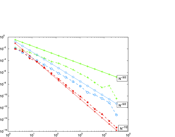
Figure 1: The lines marked by “$+$” show $N^{-3/2}$ and the standard deviation where $d=1$, the lines marked by “$\circ$” show $N^{-5/2}$ and the standard deviation where $d=2$ and the lines marked by “$*$” show $N^{-7/2}$ and the standard deviation where $d=3$.

1.2 Numerical results

Before we introduce the theoretical background, we present some simple numerical results which verify the convergence results.

Example 1.

In this example, the dimension is $1$ and the integrand is given by $f(x)=x\mathrm{e}^{x}$. Figure 1 shows the RMSE from 300 independent replications. Here, the straight lines show the functions $N^{-3/2}$, $N^{-5/2}$ and $N^{-7/2}$. The other lines are the RMSE where the digit interlacing factor $d$ is given by $1$ for the upper dashed line, $2$ for the dashed line in the middle and $3$ for the lowest of the dashed lines. Figure 1 shows that in each case the RMSE converges approximately with order $N^{-d-1/2}$ (for large enough $N$). (The result for $d=1$ appears to perform even better than $N^{-3/2}$.)

Example 2.

We consider now a two-dimensional example where the integrand is given by $f(x,y)=\frac{y\mathrm{e}^{xy}}{\mathrm{e}-2}$. This function was also used in Owenannstat2 where the sample points are obtained by scrambling and local antithetic sampling.

Figure 2 shows again the RMSE for $300$ independent replications. The straight lines show the functions $N^{-3/2}$ and $N^{-5/2}$. The two dashed lines show the RMSE when $d=1$ (upper dashed line) and when $d=2$ (lower dashed line). Figure 2 shows that in each case the RMSE converges approximately with order $N^{-d-1/2}$ (for large enough $N$).

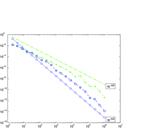
Figure 2: The lines marked by “$+$” show $N^{-3/2}$ and the standard deviation where $d=1$, the lines marked by “$\circ$” show $N^{-5/2}$ and the standard deviation where $d=2$.

In the following section, we give the necessary background on QMC, digital nets, scrambling and Walsh functions. We then prove in Section 3 what can be observed from the numerical results, namely, that if the integrand has square integrable partial mixed derivatives of order $\alpha$ in each variable, then we obtain a convergence of the RMSE of $\mathcal{O}(N^{-\min(\alpha,d)-1/2+\varepsilon})$ for any $\varepsilon>0$. A short discussion of the results is presented in Section 4. Some properties of the digit interlacing function $\mathscr{D}_{d}$ necessary for the proof is presented in Appendix A and a technical proof on the convergence of the Walsh coefficients is presented in Appendix B.

2 Background and notation

In this section, we give the necessary background on QMC methods. Some notation is required, which we now present. Here, $c,C>0$ stand for generic constants which may differ in different places. Throughout the paper, we assume that $b\geq 2$ is a prime number. We always have $\mathbf{k}=(k_{1},\ldots,k_{s})$, $\mathbf{k}^{\prime}=(k^{\prime}_{1},\ldots,k^{\prime}_{s})$, $\mathbf{x}=(x_{1},\ldots,x_{s})$, $\mathbf{y}=(y_{1},\ldots,y_{s})$, $\mathbf{x}_{n}=(x_{n,1},\ldots,x_{n,s})$, $\mathbf{y}_{n}=(y_{n,1},\ldots,y_{n,s})$.

2.1 Quasi-Monte Carlo

QMC algorithms $\widehat{I}(f)=\frac{1}{N}\sum_{n=0}^{N-1}f(\mathbf{x}_{n})$ are used to approximate integrals $I(f)=\int_{[0,1]^{s}}f(\mathbf{x})\,\mathrm{d}\mathbf{x}$. The difference to Monte Carlo is the method by which the sample points $\mathbf{x}_{0},\ldots,\mathbf{x}_{N-1}\in[0,1)^{s}$ are chosen. The aim of QMC is to chose those points such that the integration error

$$\Biggl{|}\int_{[0,1]^{s}}f(\mathbf{x})\,\mathrm{d}\mathbf{x}-\frac{1}{N}\sum_{n=0}^{N-1}f(\mathbf{x}_{n})\Biggr{|}$$

achieves the (almost) optimal rate of convergence as $N\to\infty$ for a class of functions $f\dvtx[0,1]^{s}\to\mathbb{R}$. For instance, for the set of all such functions $f$ which have bounded variation in the sense of Hardy and Krause, which we write as $\|f\|_{\mathrm{HK}}<\infty$, it is known that the best rate of convergence for the worst case error is

$$e=\sup_{f,\|f\|_{\mathrm{HK}}<\infty}\Biggl{|}\int_{[0,1]^{s}}f(\mathbf{x})\,\mathrm{d}\mathbf{x}-\frac{1}{N}\sum_{n=0}^{N-1}f(\mathbf{x}_{n})\Biggr{|}\asymp N^{-1+\varepsilon}\qquad\mbox{for all }\varepsilon>0.$$

(More precisely, there are constants $c,C>0$ such that $cN^{-1}(\log N)^{(s-1)/2}\leq e\leq CN^{-1}(\log N)^{s-1}$; see DP09 .)

Choosing the points $\mathbf{x}_{0},\ldots,\mathbf{x}_{N-1}\in[0,1)^{s}$ i.i.d. uniformly distributed as in MC does not yield this rate of convergence. Even if a function has bounded variation in the sense of Hardy and Krause one obtains only a convergence of order $N^{-1/2}$ for i.i.d. uniformly distributed sample points.

There is an explicit construction of the sample points $\mathbf{x}_{0},\ldots,\mathbf{x}_{N-1}$ for which the optimal rate of convergence is achieved. The essential insight is that the quadrature points need to be more uniformly distributed than what one obtains by choosing the sample points by chance. One criterion for how uniformly a set of points $P_{N}=\{\mathbf{x}_{0},\ldots,\mathbf{x}_{N-1}\}$ is distributed is the star discrepancy

$$D_{N}^{\ast}(P_{N})=\sup_{\mathbf{z}\in[0,1]^{s}}\Biggl{|}\frac{1}{N}\sum_{n=0}^{N-1}1_{\mathbf{x}_{i}\in[\bolds{0},\mathbf{z})}-\operatorname{Vol}([\bolds{0},\mathbf{z}))\Biggr{|},$$

where $[\bolds{0},\mathbf{z})=\prod_{i=1}^{s}[0,z_{i})$ with $\mathbf{z}=(z_{1},\ldots,z_{s})$, $\operatorname{Vol}([\bolds{0},\mathbf{z}))=\prod_{i=1}^{s}z_{i}$, the volume of $[\bolds{0},\mathbf{z})$ and

$$1_{\mathbf{x}_{i}\in[\bolds{0},\mathbf{z})}=\cases{1,&\quad if $\mathbf{x}_{i}\in[\bolds{0},\mathbf{z})$,\cr 0,&\quad otherwise.}$$

When $s=1$, this becomes the Kolmogorov–Smirnov distance between the empirical distribution of the points and the uniform distribution. Further, we call

$$\delta_{P_{N}}(\mathbf{z})=\frac{1}{N}\sum_{n=0}^{N-1}1_{\mathbf{x}_{i}\in[\bolds{0},\mathbf{z})}-\operatorname{Vol}([\bolds{0},\mathbf{z}))$$

the local discrepancy (of $P_{N}$).

The connection of this criterion to the integration error is given by the Koksma–Hlawka inequality

$$\Biggl{|}\int_{[0,1]^{s}}f(\mathbf{x})\,\mathrm{d}\mathbf{x}-\frac{1}{N}\sum_{n=0}^{N-1}f(\mathbf{x}_{n})\Biggr{|}\leq D_{N}^{\ast}(P_{N})\|f\|_{\mathrm{HK}}.$$

An explicit construction of point sets $P_{N}=\{\mathbf{x}_{0},\ldots,\mathbf{x}_{N-1}\}\in[0,1)^{s}$ for which $D^{\ast}_{N}(P_{N})\leq CN^{-1}(\log N)^{s-1}$ is given by the concept of digital nets, which we introduce in the next subsection. Notice that for such a point set, the Koksma–Hlawka inequality implies the optimal rate of convergence of the integration error, since for a given integrand, the variation $\|f\|_{\mathrm{HK}}$ does not depend on $P_{N}$ and $N$.

2.2 Digital nets

We introduce the basic ideas of digital nets in the following. A comprehensive introduction to digital nets can be found in DP09 , niedsiam . The aim is to construct a point set $P_{N}=\{\mathbf{x}_{0},\ldots,\mathbf{x}_{N-1}\}$ such that the star discrepancy satisfies $D^{\ast}_{N}(P_{N})\leq CN^{-1}(\log N)^{s-1}$. To do so, we discretize the problem by choosing the point set $P_{N}$ such that the local discrepancy $\delta_{P_{N}}(\mathbf{z})=0$ for certain $\mathbf{z}\in[0,1]^{s}$ (those $\mathbf{z}$ in turn are chosen such that the star discrepancy of $P_{N}$ is small, as we explain below).

It turns out that, when one chooses a base $b\geq 2$ and $N=b^{m}$, then for every natural number $m$ there exist point sets $P_{b^{m}}=\{\mathbf{x}_{0},\ldots,\mathbf{x}_{b^{m}-1}\}$ such that $\delta_{P_{b^{m}}}(\mathbf{z})=0$ for all $\mathbf{z}=(z_{1},\ldots,z_{s})$ of the form

$$z_{i}=\frac{a_{i}}{b^{d_{i}}}\qquad\mbox{for }1\leq i\leq s,$$

where $0<a_{i}\leq b^{d_{i}}$ is an integer and $d_{1}+\cdots+d_{s}\leq m-t$ with $d_{1},\ldots,d_{s}\geq 0$. Crucially, the value of $t$ can be chosen independently of $m$ (but dependent on $s$). A point set $P_{N}$ which satisfies this property is called a $(t,m,s)$-net in base $b$. An equivalent description of $(t,m,s)$-nets in base $b$ is given in the following definition.

Definition 1.

Let $b\geq 2$, $m,s\geq 1$ and $t\geq 0$ be integers. A point set $P_{b^{m}}=\{\mathbf{x}_{0},\ldots,\mathbf{x}_{b^{m}-1}\}\subset[0,1)^{s}$ is called a $(t,m,s)$-net in base $b$, if for all nonnegative integers $d_{1},\ldots,d_{s}$ with $d_{1}+\cdots+d_{s}=m-t$, the elementary interval

$$\prod_{i=1}^{s}\biggl{[}\frac{a_{i}}{b^{d_{i}}},\frac{a_{i}+1}{b^{d_{i}}}\biggr{)}$$

contains exactly $b^{t}$ points of $P_{b^{m}}$ for all integers $0\leq a_{i}<b^{d_{i}}$.

It can be shown that a $(t,m,s)$-net in base $b$ satisfies

$$D^{\ast}_{N}(P_{N})\leq C\frac{m^{s-1}}{b^{m-1}};$$

see DP09 , niedsiam for details. Explicit constructions of $(t,m,s)$-nets can be obtained using the digital construction scheme. Such point sets are then called digital nets [or digital $(t,m,s)$-nets if the point set is a $(t,m,s)$-net].

To describe the digital construction scheme, let $b$ be a prime number and let $\mathbb{Z}_{b}$ be the finite field of order $b$ (a prime power and the finite field $\mathbb{F}_{b}$ could be used as well). Let $C_{1},\ldots,C_{s}\in\mathbb{Z}_{b}^{dm\times m}$ be $s$ matrices of size $dm\times m$ with elements in $\mathbb{Z}_{b}$ and $d\in\mathbb{N}$. The $i$th coordinate $x_{n,i}$ of the $n$th point $\mathbf{x}_{n}=(x_{n,1},\ldots,x_{n,s})$ of the digital net is obtained in the following way. For $0\leq n<b^{m}$ let $n=n_{0}+n_{1}b+\cdots+n_{m-1}b^{m-1}$ be the base $b$ representation of $n$. Let $\vec{n}=(n_{0},\ldots,n_{m-1})^{\top}\in\mathbb{Z}_{b}^{m}$ denote the vector of digits of $n$. Then let

$$\vec{y}_{n,i}=C_{i}\vec{n}.$$

For $\vec{y}_{n,i}=(y_{n,i,1},\ldots,y_{n,i,dm})^{\top}\in\mathbb{Z}_{b}^{dm}$, we set

$$x_{n,i}=\frac{y_{n,i,1}}{b}+\cdots+\frac{y_{n,i,dm}}{b^{dm}}.$$

The construction described here is slightly more general to the classical concept to suit our needs (the classical construction scheme uses $d=1$). In this framework, we have that if $\{\mathbf{x}_{0},\ldots,\mathbf{x}_{b^{m}-1}\}$ is a digital $(t,m,ds)$-net, then $\{\mathscr{D}_{d}(\mathbf{x}_{0}),\ldots,\mathscr{D}_{d}(\mathbf{x}_{b^{m}-1})\}$ is a digital $(t,m,s)$-net; see D09 , Proposition 1.

The search for $(t,m,s)$-nets has now been reduced to finding suitable matrices $C_{1},\ldots,C_{s}$. Explicit constructions of such matrices are available; see DP09 , niedsiam .

2.3 Walsh functions

To analyze the RMSE, we use the Walsh series expansions of the integrands. In this subsection, we recall some basic properties of Walsh functions used in this paper. First, we give the definition for the one-dimensional case.

Definition 2.

Let $b\geq 2$ be an integer and represent $k\in\mathbb{N}_{0}$ in base $b$, $k=\kappa_{a-1}b^{a-1}+\cdots+\kappa_{0}$, with $\kappa_{i}\in\{0,\dots,b-1\}$. Further let $\omega_{b}=\mathrm{e}^{2\pi i/b}$. Then the $k$th Walsh function ${}_{b}{\mathrm{wal}}_{k}\dvtx[0,1)\rightarrow\{1,\omega_{b},\dots,\omega^{b-1}_{b}\}$ in base $b$ is given by

$${}_{b}{\mathrm{wal}}_{k}(x)=\omega^{x_{1}\kappa_{0}+\cdots+x_{a}\kappa_{a-1}}_{b}$$

for $x\in[0,1)$ with base $b$ representation $x=x_{1}b^{-1}+x_{2}b^{-2}+\cdots$ (unique in the sense that infinitely many of the $x_{i}$ are different from $b-1$).

We now extend this definition to the multi-dimensional case.

Definition 3.

For dimension $s\geq 2$, $\mathbf{x}=(x_{1},\dots,x_{s})\in[0,1)^{s}$ and $\mathbf{k}=(k_{1},\dots,k_{s})\in\mathbb{N}^{s}_{0}$, we define ${}_{b}{\mathrm{wal}}_{\mathbf{k}}\dvtx[0,1)^{s}\rightarrow\{1,\omega_{b},\dots,\omega^{b-1}_{b}\}$ by

$${}_{b}{\mathrm{wal}}_{\mathbf{k}}(\mathbf{x})=\prod^{s}_{j=1}{}_{b}{\mathrm{wal}}_{k_{j}}(x_{j}).$$

As can be seen from the definition, Walsh functions are piecewise constant. For $b=2$, they are also related to Haar functions.

We need some notation to introduce some further properties of Walsh functions. By $\oplus$, we denote the digitwise addition modulo $b$, that is, for $x,y\in[0,1)$ with base $b$ expansions $x=\sum^{\infty}_{i=1}x_{i}b^{-i}$ and $y=\sum^{\infty}_{i=1}y_{i}b^{-i}$, we define

$$x\oplus y=\sum^{\infty}_{i=1}z_{i}b^{-i},$$

where $z_{i}\in\{0,\dots,b-1\}$ is given by $z_{i}\equiv x_{i}+y_{i}(\operatorname{mod}b)$, and let $\ominus$ denote the digitwise subtraction modulo $b$. In the same manner, we also define a digitwise addition and digitwise subtraction for nonnegative integers based on the $b$-adic expansion. For vectors in $[0,1)^{s}$ or $\mathbb{N}^{s}_{0}$, the operators $\oplus$ and $\ominus$ are carried out componentwise. Throughout this paper, we always use base $b$ for the operations $\oplus$ and $\ominus$. Further we call $x\in[0,1)$ a $b$-adic rational if it can be written in a finite base $b$ expansion. In the following proposition, we summarize some basic properties of Walsh functions.

Proposition 4

1. For all $k,l\in\mathbb{N}_{0}$ and all $x,y\in[0,1)$, with the restriction that if $x,y$ are not $q$-adic rationals, then $x\oplus y$ is not allowed to be a $b$-adic rational, we have

   $${}_{b}{\mathrm{wal}}_{k}(x)\cdot{}_{b}{\mathrm{wal}}_{l}(x)=\mathrm{wal}_{k\oplus l}(x),\qquad{}_{b}{\mathrm{wal}}_{k}(x)\cdot{}_{b}{\mathrm{wal}}_{k}(y)={}_{b}{\mathrm{wal}}_{k}(x\oplus y).$$

2. We have

   $$\int^{1}_{0}{}_{b}{\mathrm{wal}}_{0}(x)\,\mathrm{d}x=1\quad\mbox{and}\quad\int^{1}_{0}{}_{b}{\mathrm{wal}}_{k}(x)\,\mathrm{d}x=0\qquad\mbox{if }k>0.$$

3. For all $\mathbf{k},\mathbf{l}\in\mathbb{N}^{s}_{0}$, we have the following orthogonality properties:

   $$\int_{[0,1)^{s}}{}_{b}{\mathrm{wal}}_{\mathbf{k}}(\mathbf{x})\overline{{}_{b}{\mathrm{wal}}_{\mathbf{l}}(\mathbf{x})}\,\mathrm{d}\mathbf{x}=\cases{1,&\quad if $\mathbf{k}=\mathbf{l}$,\cr 0,&\quad otherwise.}$$

4. For any $f\in\mathcal{L}_{2}([0,1)^{s})$ and any $\bolds{\sigma}\in[0,1)^{s}$, we have

   $$\int_{[0,1)^{s}}f(\mathbf{x}\oplus\bolds{\sigma})\,\mathrm{d}\mathbf{x}=\int_{[0,1)^{s}}f(\mathbf{x})\,\mathrm{d}\mathbf{x}.$$

5. For $s\in\mathbb{N}$, the system $\{{}_{b}{\mathrm{wal}}_{\mathbf{k}}\dvtx\mathbf{k}=(k_{1},\dots,k_{s}),k_{1},\dots,k_{s}\geq 0\}$ is a complete orthonormal system in $\mathcal{L}_{2}([0,1]^{s})$.

The proofs of 1–3 are straightforward, and for a proof of the remaining items see ChrestensonWalsh or DP09 , WalshClSeNo for more information.

Let $d\geq 1$ and $k_{1},\ldots,k_{d}\in\mathbb{N}_{0}$. Let $k_{i}=\kappa_{i,0}+\kappa_{i,1}b+\cdots$, where $\kappa_{i,a}\in\{0,\ldots,b-1\}$ and $\kappa_{i,a}=0$ for $a$ large enough. To analyze the RMSE, it is convenient to define a digit interlacing function $\mathscr{E}_{d}$ for natural numbers, that is,

$$\mathscr{E}_{d}\dvtx\mathbb{N}^{d} \to \mathbb{N},$$

$$(k_{1},\ldots,k_{d}) \mapsto \sum_{a=0}^{\infty}\sum_{r=1}^{d}\kappa_{r,a}b^{r-1+ad}.$$

We also extend this function to vectors

$$\mathscr{E}_{d}\dvtx\mathbb{N}^{ds} \to \mathbb{N}^{s},$$

$$(k_{1},\ldots,k_{ds}) \mapsto \bigl{(}\mathscr{E}_{d}(k_{1},\ldots,k_{d}),\ldots,\mathscr{E}_{d}\bigl{(}k_{d(s-1)+1},\ldots,k_{ds}\bigr{)}\bigr{)}.$$

Then we have

$${}_{b}{\mathrm{wal}}_{\mathscr{E}_{d}(k_{1},\ldots,k_{d})}(\mathscr{D}_{d}(x_{1},\ldots,x_{d}))=\prod_{i=1}^{d}{}_{b}{\mathrm{wal}}_{k_{i}}(x_{i}).$$

2.4 Scrambling

The scrambling algorithm which yields the optimal rate of convergence of the RMSE uses the digit interlacing function and the scrambling introduced by Owen Owenproc , Owensiam , Owenannstat , which we describe in the following.

2.4.1 Owen’s scrambling

Owen’s scrambling algorithm is easiest described for some generic point $\mathbf{x}\in[0,1)^{s}$, with $\mathbf{x}=(x_{1},\ldots,x_{s})$ and $x_{i}=\xi_{i,1}b^{-1}+\xi_{i,2}b^{-2}+\cdots$. The scrambled point shall be denoted by $\mathbf{y}\in[0,1)^{s}$, where $\mathbf{y}=(y_{1},\dots,y_{s})$ and $y_{i}=\eta_{i,1}b^{-1}+\eta_{i,2}b^{-2}+\cdots$. The point $\mathbf{y}$ is obtained by applying permutations to each digit of each coordinate of $\mathbf{x}$. The permutation applied to $\xi_{i,l}$ depends on $\xi_{i,k}$ for $1\leq k<l$. Specifically, $\eta_{i,1}=\pi_{i}(\xi_{i,1})$, $\eta_{i,2}=\pi_{i,\xi_{i,1}}(\xi_{i,2})$, $\eta_{i,3}=\pi_{i,\xi_{i,1},\xi_{i,2}}(\xi_{i,3})$, and in general

$$\eta_{i,k}=\pi_{i,\xi_{i,1},\dots,\xi_{i,k-1}}(\xi_{i,k}),$$ (1)

where $\pi_{i,\xi_{i,1},\dots,\xi_{i,k-1}}$ is a random permutation of $\{0,\dots,b-1\}$. We assume that permutations with different indices are chosen mutually independent from each other and that each permutation is chosen with the same probability.

To describe Owen’s scrambling, for $1\leq i\leq s$ let

$$\Pi_{i}=\bigl{\{}\pi_{i,\xi_{i,1},\dots\xi_{i,k-1}}\dvtx k\in{\mathbb{N}},\xi_{i,1},\ldots,\xi_{i,k-1}\in\{0,\ldots,b-1\}\bigr{\}},$$

where for $k=1$ we set $\pi_{i,\xi_{i,1},\dots,\xi_{i,k-1}}=\pi_{i}$, be a given set of permutations and let $\bolds{\Pi}=(\Pi_{1},\ldots,\Pi_{s})$. Then, when applying Owen’s scrambling using these permutations to some point $\mathbf{x}\in[0,1)^{s}$, we write $\mathbf{y}=\bolds{\Pi}(\mathbf{x})$, where $\mathbf{y}$ is the point obtained by applying Owen’s scrambling to $\mathbf{x}$ using the set of permutations $\bolds{\Pi}=(\Pi_{1},\ldots,\Pi_{s})$. For $x\in[0,1)$ we drop the subscript $i$ and just write $y=\Pi(x)$.

2.4.2 Owen’s scrambling of order $d$

To analyze the RMSE it is also convenient to generalize Owen’s scrambling to higher order. We now describe what we mean by Owen’s scrambling of order $d\geq 1$ for a generic point $\mathbf{x}\in[0,1)^{s}$. The scrambled point $\mathbf{y}\in[0,1)^{s}$ is given by

$$\mathbf{y}=\mathscr{D}_{d}(\bolds{\Pi}(\mathscr{D}_{d}^{-1}(\mathbf{x}))),$$

that is, one applies the inverse mapping $\mathscr{D}_{d}^{-1}$ (see Appendix A for more information on $\mathscr{D}_{d}$) to the point $\mathbf{x}$ to obtain a point $\mathbf{z}\in[0,1)^{ds}$, applies Owen’s scrambling of Section 2.4.1 to $\mathbf{z}$ to obtain a point $\mathbf{w}=\bolds{\Pi}(\mathbf{z})\in[0,1)^{ds}$ and then use the transformation $\mathscr{D}_{d}$ to obtain the point $\mathbf{y}=\mathscr{D}_{d}(\mathbf{w})\in[0,1)^{s}$. Assuming that the permutations are all chosen with equal probability, then the point $\mathbf{y}$ is uniformly distributed in $[0,1)^{s}$.

Proposition 5

Let $\mathbf{x}\in[0,1)^{s}$ and let $\bolds{\Pi}$ be a uniformly and i.i.d. set of permutations. Then $\mathscr{D}_{d}(\bolds{\Pi}(\mathscr{D}^{-1}_{d}(\mathbf{x})))$ is uniformly distributed in $[0,1)^{s}$, that is, for any Lebesgue measurable set $G\subseteq[0,1)^{s}$, the probability that $\mathscr{D}_{d}(\bolds{\Pi}(\mathscr{D}^{-1}_{d}(\mathbf{x})))$, denoted by $\operatorname{Prob}[\mathscr{D}_{d}(\bolds{\Pi}(\mathscr{D}^{-1}_{d}(\mathbf{x})))]=\lambda_{s}(G)$, where $\lambda_{s}$ denotes the $s$-dimensional Lebesgue measure.

This result follows along the same lines as the proof of Owenproc , Proposition 2.

2.4.3 Owen’s lemma of order $d$

A key result on scrambled nets is Owen’s lemma (see Owensiam ) which we now generalize to include the case of scrambling of order $d$. Let $k\in\mathbb{N}$ have base $b$ representation $k=\kappa_{0}+\kappa_{1}b+\cdots+\kappa_{a}b^{a}$. For $0\leq r<d$ let

$$k_{r}=\kappa_{r}b^{r}+\kappa_{r+d}b^{r+d}+\cdots+\kappa_{a_{r}}b^{a_{r}},$$

where $a_{r}\leq a$ is the largest integer such that $d$ divides $a_{r}-r$. If $a<r$, we set $k_{r}=0$. For $x=\xi_{1}b^{-1}+\xi_{2}b^{-2}+\cdots$ and $x^{\prime}=\xi^{\prime}_{1}b^{-1}+\xi^{\prime}_{2}b^{-2}+\cdots$ and for $0\leq r<d$ let $\beta_{r}$ be the largest integer such that $\xi_{r}=\xi^{\prime}_{r},\xi_{r+d}=\xi^{\prime}_{r+d},\ldots,\xi_{r+\beta_{r}d}=\xi^{\prime}_{r+\beta_{r}d}$ and $\xi_{r+(\beta_{r}+1)d}\neq\xi^{\prime}_{r+(\beta_{r}+1)d}$.

Lemma 6

Let $y,y^{\prime}\in[0,1)$ be two points obtained by applying Owen’s scrambling algorithm of order $d\geq 1$ to the points $x,x^{\prime}\in[0,1)$.

• [(iii)]

• If $k\neq k^{\prime}$, then

  $${\mathbb{E}}[{}_{b}{\mathrm{wal}}_{k}(y)\overline{{}_{b}{\mathrm{wal}}_{k^{\prime}}(y^{\prime})}]=0.$$

• If $k=k^{\prime}$ and there exists an $0\leq r<d$ such that $k_{r}\geq b^{\beta_{r}+1}$, then

  $${\mathbb{E}}[{}_{b}{\mathrm{wal}}_{k}(y\ominus y^{\prime})]=0.$$

• If $k=k^{\prime}$ and $k_{r}<b^{\beta_{r}+1}$ for $0\leq r<d$, then

  $${\mathbb{E}}[{}_{b}{\mathrm{wal}}_{k}(y\ominus y^{\prime})]=(1-b)^{-v},$$

  where

  $$v=|\{0\leq r<d\dvtx b^{\beta_{r}}\leq k_{r}<b^{\beta_{r}+1}\}|.$$

The proof of this result follows immediately from DP09 , Lemma 13.23. In the next section, we analyze the variance of the estimator $\widehat{I}(f)=\frac{1}{b^{m}}\sum_{n=0}^{b^{m}-1}f(\mathbf{y}_{n})$.

3 Variance of the estimator

Let $f\in L_{2}([0,1]^{s})$ have the following Walsh series expansion

$$f(\mathbf{x})\sim\sum_{\mathbf{k}\in{\mathbb{N}}_{0}^{s}}\widehat{f}(\mathbf{k}){}_{b}{\mathrm{wal}}_{\mathbf{k}}(\mathbf{x})=:S(\mathbf{x},f).$$ (2)

Although we do not necessarily have equality in (2), the completeness of the Walsh function system $\{{}_{b}{\mathrm{wal}}_{\mathbf{k}}\dvtx\mathbf{k}\in{\mathbb{N}}_{0}^{s}\}$ (see DP09 ) implies that we do have

$$\operatorname{Var}[f]=\sum_{\mathbf{k}\in{\mathbb{N}}_{0}^{s}}|\widehat{f}(\mathbf{k})|^{2}=\operatorname{Var}[S(\cdot,f)].$$ (3)

We estimate the integral $\int_{[0,1]^{s}}f(\mathbf{x})\,\mathrm{d}\mathbf{x}$ by

$$\widehat{I}(f)=\frac{1}{b^{m}}\sum_{n=0}^{b^{m}-1}f(\mathbf{y}_{n}),$$

where $\mathbf{y}_{0},\ldots,\mathbf{y}_{b^{m}-1}\in[0,1)^{s}$ is obtained by applying a random Owen scrambling of order $d$ to the digital $(t,m,s)$-net $P_{b^{m}}=\{\mathbf{x}_{0},\ldots,\mathbf{x}_{b^{m}-1}\}$ [below we shall assume that there is a digital $(t,m,ds)$-net $\{\mathbf{z}_{0},\ldots,\mathbf{z}_{b^{m}-1}\}$ such that $\mathbf{x}_{n}=\mathscr{D}_{d}(\mathbf{z}_{n})$ for $0\leq n<b^{m}$, but for now the assumption that $P_{b^{m}}$ is a digital $(t,m,s)$-net is sufficient]. From Proposition 5, it follows that

$${\mathbb{E}}[\widehat{I}(f)]=\int_{[0,1]^{s}}f(\mathbf{x})\,\mathrm{d}\mathbf{x}.$$

Hence, in the following, we consider the variance of the estimator $\widehat{I}(f)$ denoted by

$$\operatorname{Var}[\widehat{I}(f)]={\mathbb{E}}\bigl{[}\bigl{(}\widehat{I}(f)-{\mathbb{E}}[\widehat{I}(f)]\bigr{)}^{2}\bigr{]}.$$

The following notation is needed for the lemma below. Let $d\geq 1$ and $\mathbf{l}=(\mathbf{l}_{1},\ldots,\mathbf{l}_{s})\in\mathbb{N}_{0}^{ds}$, where $\mathbf{l}_{i}=(l_{(i-1)d+1},\ldots,l_{id})$. Let

$$B_{d,\mathbf{l},s}=\{(k_{1},\ldots,k_{ds})\in\mathbb{N}_{0}^{ds}\dvtx\lfloor b^{l_{i}-1}\rfloor\leq k_{i}<b^{l_{i}}\mbox{ for }1\leq i\leq ds\}.$$

We set

$$\sigma^{2}_{d,\mathbf{l},s}(f)=\sum_{\mathbf{k}\in B_{d,\mathbf{l},s}}|\widehat{f}(\mathscr{E}_{d}(\mathbf{k}))|^{2}.$$

Consider $s=1$ for a moment. Let $\mathbf{l}\in\mathbb{N}_{0}^{d}$. Then Lemma 6 implies that for $(k_{1},\ldots,k_{d}),(k^{\prime}_{1},\ldots,k^{\prime}_{d})\in B_{d,\mathbf{l},1}$ we have

$${\mathbb{E}}\bigl{[}{}_{b}{\mathrm{wal}}_{(k_{1},\ldots,k_{d})}(\bolds{\Pi}(\mathscr{D}_{d}^{-1}(x)))\overline{{}_{b}{\mathrm{wal}}_{(k_{1},\ldots,k_{d})}(\bolds{\Pi}(\mathscr{D}_{d}^{-1}(x^{\prime})))}\bigr{]}$$

(4)

$$\qquad={\mathbb{E}}\bigl{[}{}_{b}{\mathrm{wal}}_{(k^{\prime}_{1},\ldots,k^{\prime}_{d})}(\bolds{\Pi}(\mathscr{D}_{d}^{-1}(x)))\overline{{}_{b}{\mathrm{wal}}_{(k^{\prime}_{1},\ldots,k^{\prime}_{d})}(\bolds{\Pi}(\mathscr{D}_{d}^{-1}(x^{\prime})))}\bigr{]}.$$

Hence, for $s\geq 1$ and $\mathbf{l}\in\mathbb{N}_{0}^{ds}$, choose an arbitrary $\mathbf{k}\in B_{d,\mathbf{l},s}$, and set

$$\Gamma_{d,\mathbf{l}}(P_{b^{m}}) = \frac{1}{b^{2m}}\sum_{n,n^{\prime}=0}^{b^{m}-1}\prod_{i=1}^{s}{\mathbb{E}}\bigl{[}{}_{b}{\mathrm{wal}}_{(k_{d(i-1)+1},\ldots,k_{di})}(\bolds{\Pi}(\mathscr{D}_{d}^{-1}(x_{n,i})))$$

$$\hskip 72.0pt{}\times\overline{{}_{b}{\mathrm{wal}}_{(k_{d(i-1)+1},\ldots,k_{di})}(\bolds{\Pi}(\mathscr{D}_{d}^{-1}(x_{n^{\prime},i})))}\bigr{]}.$$

Equation (3) implies that this definition is independent of the particular choice of $\mathbf{k}\in B_{d,\mathbf{l},s}$. We call $\Gamma_{d,\mathbf{l}}(P_{b^{m}})$ the gain coefficient (of $P_{b^{m}}$) (of order $d$).

Lemma 7

Let $d\geq 1$. Let $f\in L_{2}([0,1]^{s})$ and

$$\widehat{I}(f)=\frac{1}{b^{m}}\sum_{n=0}^{b^{m}-1}f(\mathbf{y}_{n}),$$

where $\mathbf{y}_{0},\ldots,\mathbf{y}_{b^{m}-1}\in[0,1)^{s}$ is obtained by applying a random Owen scrambling of order $d$ to the digital net $P_{b^{m}}=\{\mathbf{x}_{0},\ldots,\mathbf{x}_{b^{m}-1}\}$. Then

$$\operatorname{Var}[\widehat{I}(f)]=\sum_{\mathbf{l}\in\mathbb{N}_{0}^{ds}\setminus\{\bolds{0}\}}\sigma^{2}_{d,\mathbf{l},s}(f)\Gamma_{d,\mathbf{l}}(P_{b^{m}}).$$

Using the linearity of expectation and Lemma 6, we get

$$\operatorname{Var}[\widehat{I}(f)]$$

$$\qquad={\mathbb{E}}\Biggl{[}\sum_{\mathbf{k},\mathbf{k}^{\prime}\in\mathbb{N}_{0}^{s}\setminus\{\bolds{0}\}}\widehat{f}(\mathbf{k})\overline{\widehat{f}(\mathbf{k}^{\prime})}\frac{1}{b^{2m}}\sum_{n,n^{\prime}=0}^{b^{m}-1}{}_{b}{\mathrm{wal}}_{\mathbf{k}}(\mathbf{y}_{n})\overline{{}_{b}{\mathrm{wal}}_{\mathbf{k}^{\prime}}(\mathbf{y}_{n^{\prime}})}\Biggr{]}$$

$$\qquad=\sum_{\mathbf{k},\mathbf{k}^{\prime}\in\mathbb{N}_{0}^{s}\setminus\{\bolds{0}\}}\widehat{f}(\mathbf{k})\overline{\widehat{f}(\mathbf{k}^{\prime})}\frac{1}{b^{2m}}\sum_{n,n^{\prime}=0}^{b^{m}-1}\prod_{i=1}^{s}{\mathbb{E}}[{}_{b}{\mathrm{wal}}_{k_{i}}(y_{n,i})\overline{{}_{b}{\mathrm{wal}}_{k^{\prime}_{i}}(y_{n^{\prime},i})}]$$

$$\qquad=\sum_{\mathbf{k}\in\mathbb{N}_{0}^{s}\setminus\{\bolds{0}\}}|\widehat{f}(\mathbf{k})|^{2}\frac{1}{b^{2m}}\sum_{n,n^{\prime}=0}^{b^{m}-1}\prod_{i=1}^{s}{\mathbb{E}}[{}_{b}{\mathrm{wal}}_{k_{i}}(y_{n,i})\overline{{}_{b}{\mathrm{wal}}_{k_{i}}(y_{n^{\prime},i})}]$$

$$\qquad=\sum_{\mathbf{l}\in\mathbb{N}_{0}^{ds}\setminus\{\bolds{0}\}}\sum_{\mathbf{k}\in B_{d,\mathbf{l},s}}|\widehat{f}(\mathscr{E}_{d}(\mathbf{k}))|^{2}$$

$$\qquad\quad{}\times\frac{1}{b^{2m}}\sum_{n,n^{\prime}=0}^{b^{m}-1}\prod_{i=1}^{s}{\mathbb{E}}\bigl{[}{}_{b}{\mathrm{wal}}_{(k_{d(i-1)+1},\ldots,k_{di})}(\bolds{\Pi}(\mathscr{D}_{d}^{-1}(x_{n,i}))\ominus\bolds{\Pi}(\mathscr{D}_{d}^{-1}(x_{n^{\prime},i})))\bigr{]}$$

$$\qquad=\sum_{\mathbf{l}\in\mathbb{N}_{0}^{ds}\setminus\{\bolds{0}\}}\sigma^{2}_{d,\mathbf{l},s}(f)\Gamma_{d,\mathbf{l}}(P_{b^{m}}).$$

Hence, the result follows.

To obtain a bound on the variance $\operatorname{Var}[\widehat{I}(f)]$, we prove bounds on $\sigma_{d,\mathbf{l},s}(f)$ and $\Gamma_{d,\mathbf{l}}(P_{b^{m}})$, which we consider in the following two subsections.

3.1 A bound on the gain coefficients of order $d$

In this section, we prove a bound on $\Gamma_{d,\mathbf{l}}(P_{b^{m}})$, where the point set is a digital $(t,m,s)$-net as constructed in D08 .

Lemma 8

Let $\{\mathbf{z}_{0},\ldots,\mathbf{z}_{b^{m}-1}\}$ be a digital $(t,m,ds)$-net over $\mathbb{Z}_{b}$. Let $\mathbf{x}_{n}=\mathscr{D}_{d}(\mathbf{z}_{n})$ for $0\leq n<b^{m}$. Then the gain coefficients of order $d$ for the digital net $P_{b^{m}}=\{\mathbf{x}_{0},\ldots,\mathbf{x}_{b^{m}-1}\}$ satisfy

$$\Gamma_{d,\mathbf{l}}(P_{b^{m}})\leq\cases{0,&\quad if $|\mathbf{l}|_{1}\leq m-t$,\cr b^{|q|-|\mathbf{l}|_{1}},&\quad if $m-t<|\mathbf{l}|_{1}\leq m-t+|q|$,\cr b^{-m+t},&\quad if $|\mathbf{l}|_{1}>m-t+|q|$.}$$

Let $\mathbf{k}=(k_{1},\ldots,k_{ds})$ and $\mathbf{l}=(\mathbf{l}_{q},\bolds{0})$ for some $q\subseteq\{1,\ldots,s\}$. Then from the proof of DP09 , Corollary 13.7 and DP09 , Lemma 13.8, it follows that

$$\Gamma_{d,\mathbf{l}}(P_{b^{m}}) = \frac{1}{b^{2m}}\sum_{n,n^{\prime}=0}^{b^{m}-1}\prod_{i=1}^{s}{\mathbb{E}}\bigl{[}{}_{b}{\mathrm{wal}}_{(k_{d(i-1)+1},\ldots,k_{di})}(\bolds{\Pi}(\mathscr{D}_{d}^{-1}(x_{n,i})))$$

$$\hskip 71.0pt{}\times\overline{{}_{b}{\mathrm{wal}}_{(k^{\prime}_{d(i-1)+1},\ldots,k^{\prime}_{di})}(\bolds{\Pi}(\mathscr{D}_{d}^{-1}(x_{n^{\prime},i})))}\bigr{]}$$

$$= \frac{1}{b^{2m}}\sum_{n,n^{\prime}=0}^{b^{m}-1}\prod_{i=1}^{s}{\mathbb{E}}[{}_{b}{\mathrm{wal}}_{\mathbf{k}}(\bolds{\Pi}(\mathbf{z}_{n}))\overline{{}_{b}{\mathrm{wal}}_{\mathbf{k}}(\bolds{\Pi}(\mathbf{z}_{n^{\prime}}))}]$$

$$= \cases{0,&\quad if $|\mathbf{l}|_{1}\leq m-t$,\cr b^{|q|-|\mathbf{l}|_{1}},&\quad if $m-t<|\mathbf{l}|_{1}\leq m-t+|q|$,\cr b^{-m+t},&\quad if $|\mathbf{l}|_{1}>m-t+|q|$.}$$

Hence, the result follows.

3.2 Higher order variation

In this subsection, we state a bound on $\sigma_{d,\mathbf{l},s}(f)$. The rate of decay of $\sigma_{d,\mathbf{l},s}(f)$ depends on the smoothness of the function $f$. We measure the smoothness using a variation based on finite differences, which we introduce in the following. Since the smoothness of the function $f$ may be unknown, we cannot assume that we can choose $d$ to be the smoothness. Hence, in the following we use $\alpha$ to denote the smoothness of the integrand $f$.

3.2.1 Finite differences

We use a slight variation from classical finite differences. Let $f\dvtx[0,1]\to\mathbb{R}$ and let $z_{1},z_{2},\ldots\in(-1,1)$ be a sequence of numbers. Then we define $\Delta_{0}(x)f=f(x)$ and for $\alpha\geq 1$ we set

$$\Delta_{\alpha}(x;z_{1},\ldots,z_{\alpha})f=\Delta_{\alpha-1}(x+z_{\alpha};z_{1},\ldots,z_{\alpha-1})f-\Delta_{\alpha-1}(x;z_{1},\ldots,z_{\alpha-1})f.$$

For instance, we have

$$\Delta_{1}(x;z_{1})f = f(x+z_{1})-f(x),$$

$$\Delta_{2}(x;z_{1},z_{2})f = f(x+z_{1}+z_{2})-f(x+z_{2})-f(x+z_{1})+f(x),$$

and in general

$$\Delta_{\alpha}(x;z_{1},\ldots,z_{\alpha})f=\sum_{v\subseteq\{1,\ldots,\alpha\}}(-1)^{|v|}f\biggl{(}x+\sum_{i\in v}z_{i}\biggr{)},$$

where $|v|$ denotes the number of elements in $v$. We always assume that $x+\sum_{i\in v}z_{i}\in[0,1]$ for all $v\subseteq\{1,\ldots,\alpha\}$.

If $f$ is $\alpha$ times continuously differentiable, then the mean value theorem implies that

$$\Delta_{\alpha}(x;z_{1},\ldots,z_{\alpha})f=z_{\alpha}\Delta_{\alpha-1}(\zeta_{1};z_{1},\ldots,z_{\alpha-1})\frac{\mathrm{d}f}{\mathrm{d}x},$$

where $\min(x,x+z_{\alpha})\leq\zeta_{1}\leq\max(x,x+z_{\alpha})$. By induction, it then follows that

$$\Delta_{\alpha}(x;z_{1},\ldots,z_{\alpha})f=z_{1}\cdots z_{\alpha}\frac{\mathrm{d}^{\alpha}f}{\mathrm{d}x^{\alpha}}(\zeta_{\alpha}),$$

where

$$x+\min_{v\subseteq\{1,\ldots,\alpha\}}\sum_{i\in v}z_{i}\leq\zeta_{\alpha}\leq x+\max_{v\subseteq\{1,\ldots,\alpha\}}\sum_{i\in v}z_{i}.$$

We generalize the difference operator to functions $f\dvtx[0,1]^{s}\to\mathbb{R}$. Let $\alpha>0$ be a nonnegative integer. Let $\Delta_{i,\alpha}$ be the one-dimensional difference operator $\Delta_{\alpha}$ applied to the $i$th coordinate of $f$. For $\bolds{\alpha}=(\alpha_{1},\ldots,\alpha_{s})\in\{0,\ldots,\alpha\}^{s}$ and $1\leq i\leq s$ let $z_{i,1},\ldots,z_{i,\alpha_{i}}\in(-1,1)$. Then we define

$$\Delta_{\bolds{\alpha}}(\mathbf{x};(z_{1,1},\ldots,z_{1,\alpha_{1}}),\ldots,(z_{s,1},\ldots,z_{s,\alpha_{s}}))f$$

$$\qquad=\Delta_{1,\alpha_{1}}(x_{1};z_{1,1},\ldots,z_{1,\alpha_{1}})\cdots\Delta_{s,\alpha_{s}}(x_{s};z_{s,1},\ldots,z_{s,\alpha_{s}})f$$

$$\qquad=\sum_{v_{1}\subseteq\{1,\ldots,\alpha_{1}\}}\cdots\sum_{v_{s}\subseteq\{1,\ldots,\alpha_{s}\}}(-1)^{|v_{1}|+\cdots+|v_{s}|}$$

$$\hskip 136.5pt{}\times f\biggl{(}x_{1}+\sum_{i_{1}\in v_{1}}z_{1,i_{1}},\ldots,x_{s}+\sum_{i_{s}\in v_{s}}z_{s,i_{s}}\biggr{)}.$$

If $f$ has continuous mixed partial derivatives up to order $\alpha$ in each variable, then, as for the one-dimensional case, we have

$$\Delta_{\bolds{\alpha}}(\mathbf{x},(z_{1,1},\ldots,z_{1,\alpha_{1}}),\ldots,(z_{s,1},\ldots,z_{s,\alpha_{s}}))f$$

(5)

$$\qquad=\prod_{i=1}^{s}\prod_{r_{i}=1}^{\alpha_{i}}z_{i,r_{i}}\frac{\partial^{\alpha_{1}+\cdots+\alpha_{s}}f}{\partial x_{1}^{\alpha_{1}}\cdots\partial x_{s}^{\alpha_{s}}}(\zeta_{1,\alpha_{1}},\ldots,\zeta_{s,\alpha_{s}}),$$

where we set $\prod_{r_{i}=1}^{\alpha_{i}}z_{i,r_{i}}=1$ for $\alpha_{i}=0$ and where

$$x_{i}+\min_{v\subseteq\{1,\ldots,\alpha_{i}\}}\sum_{r\in v}z_{i,r}\leq\zeta_{i,\alpha_{i}}\leq x_{i}+\max_{v\subseteq\{1,\ldots,\alpha_{i}\}}\sum_{r\in v}z_{i,r}$$

for $1\leq i\leq s$. Again we assume that $x_{i}+\sum_{r\in v}z_{i,r}\in[0,1]$ for all $v\subseteq\{1,\ldots,\alpha_{i}\}$, $\zeta_{i,\alpha_{i}}\in[0,1]$ for all $0\leq\alpha_{i}\leq\alpha$ and $1\leq i\leq s$.

3.2.2 Variation

Let $f\dvtx[0,1]^{s}\to\mathbb{R}$ and $\alpha>0$ be a nonnegative integer. Let $J=\prod_{i=1}^{\alpha s}[\frac{a_{i}}{b^{l_{i}}},\frac{a_{i}+1}{b^{l_{i}}})$, with $0\leq a_{i}<b^{l_{i}}$ and $l_{i}\in\mathbb{N}$ for $1\leq i\leq\alpha s$. Apart from at most a countable number of points, the set $\mathscr{D}_{\alpha}(J)$ is the product of a union of intervals. Let $\bolds{\alpha}=(\alpha_{1},\ldots,\alpha_{s})\in\{1,\ldots,\alpha\}^{s}$. Then we define the generalized Vitali variation by

$$V_{\bolds{\alpha}}^{(s)}(f)=\sup_{\mathcal{P}}\biggl{(}\sum_{J\in\mathcal{P}}\operatorname{Vol}(\mathscr{D}_{\alpha}(J))\sup\biggl{|}\frac{\Delta_{\bolds{\alpha}}(\mathbf{t};\mathbf{z}_{1},\ldots,\mathbf{z}_{s})f}{\prod_{i=1}^{s}\prod_{r=1}^{\alpha_{i}}z_{i,r}}\biggr{|}^{2}\biggr{)}^{1/2},$$ (6)

where the first supremum $\sup_{\mathcal{P}}$ is extended over all partitions of $[0,1)^{\alpha s}$ into subcubes of the form $J=\prod_{i=1}^{\alpha s}[\frac{a_{i}}{b^{l_{i}}},\frac{a_{i}+1}{b^{l_{i}}})$ with $0\leq a_{i}<b^{l_{i}}$ and $l_{i}\in\mathbb{N}$ for $1\leq i\leq\alpha s$, and the second supremum is taken over all $\mathbf{t}\in\mathscr{D}_{\alpha}(J)$ and $\mathbf{z}_{i}=(z_{i,1},\ldots,z_{i,\alpha_{i}})$ with $z_{i,r}=\tau_{i,r}b^{-\alpha(l_{i}-1)-r}$ where $\tau_{i,r}\in\{1-b,\ldots,b-1\}\setminus\{0\}$ for $1\leq r\leq\alpha_{i}$ and $1\leq i\leq s$ and such that all the points at which $f$ is evaluated in $\Delta_{\alpha}(\mathbf{t};\mathbf{z}_{1},\ldots,\mathbf{z}_{s})$ are in $\mathscr{D}_{\alpha}(\prod_{i=1}^{\alpha s}[b^{-l_{i}+1}\lfloor a_{i}/b\rfloor,b^{-l_{i}+1}(\lfloor a_{i}/b\rfloor+1))$.

In Appendix A it is shown that $\operatorname{Vol}(\mathscr{D}_{\alpha}(J))=\operatorname{Vol}(J)$, the volume (i.e., Lebesgue measure) of $J$. Hence, if the partial derivative $\frac{\partial^{\alpha_{1}+\cdots+\alpha_{s}}f}{\partial x_{1}^{\alpha_{1}}\cdots\partial x_{s}^{\alpha_{s}}}$ are continuous for a given $(\alpha_{1},\ldots,\alpha_{s})\in\{1,\ldots,\alpha\}^{s}$, then it can be shown that (3.2.1) and the mean value theorem imply that the sum (6) is a Riemann sum for the integral

$$V_{\bolds{\alpha}}^{(s)}(f)=\biggl{(}\int_{[0,1]^{s}}\biggl{|}\frac{\partial^{\alpha_{1}+\cdots+\alpha_{s}}f}{\partial x_{1}^{\alpha_{1}}\cdots\partial x_{s}^{\alpha_{s}}}(\mathbf{x})\biggr{|}^{2}\,\mathrm{d}\mathbf{x}\biggr{)}^{1/2}.$$

For $\varnothing\neq u\subseteq\{1,\ldots,s\}$, let $|u|$ denote the number of elements in the set $u$ and let $V_{\bolds{\alpha}_{u}}^{(|u|)}(f_{u};u)$ be the generalized Vitali variation with coefficient $\bolds{\alpha}_{u}\in\{1,\ldots,\alpha\}^{|u|}$ of the $|u|$-dimensional function

$$f_{u}(\mathbf{x}_{u})=\int_{[0,1]^{s-|u|}}f(\mathbf{x})\,\mathrm{d}\mathbf{x}_{\{1,\ldots,s\}\setminus u}.$$

For $u=\varnothing$, we have $f_{\varnothing}=\int_{[0,1]^{s}}f(\mathbf{x})\,\mathrm{d}\mathbf{x}$ and we define $V_{\bolds{\alpha}}^{(|\varnothing|)}(f_{\varnothing};\varnothing)=|f_{\varnothing}|$.

Then

$$V_{\alpha}(f)=\biggl{(}\sum_{u\subseteq\{1,\ldots,s\}}\sum_{\bolds{\alpha}\in\{1,\ldots,\alpha\}^{|u|}}\bigl{(}V_{\bolds{\alpha}}^{(|u|)}(f_{u};u)\bigr{)}^{2}\biggr{)}^{1/2}$$

is called the generalized Hardy and Krause variation of $f$ of order $\alpha$. A function $f$ for which $V_{\alpha}(f)$ is finite is said to be of bounded variation (of order $\alpha$).

If the partial derivatives $\frac{\partial^{\alpha_{1}+\cdots+\alpha_{s}}f}{\partial x_{1}^{\alpha_{1}}\cdots\partial x_{s}^{\alpha_{s}}}$ are continuous for all $(\alpha_{1},\ldots,\alpha_{s})\in\{0,\ldots,\alpha\}^{s}$, then variation coincides with the norm

$$V_{\alpha}(f)=\biggl{(}\sum_{u\subseteq\{1,\ldots,s\}}\sum_{\bolds{\alpha}\in\{1,\ldots,\alpha\}^{|u|}}\int_{[0,1]^{|u|}}\biggl{|}\int_{[0,1]^{s-|u|}}\frac{\partial^{\sum_{i\in u}\alpha_{i}}f}{\prod_{i\in u}\partial x_{i}^{\alpha_{i}}}\,\mathrm{d}\mathbf{x}_{\{1,\ldots,s\}\setminus u}\biggr{|}^{2}\,\mathrm{d}\mathbf{x}_{u}\biggr{)}^{1/2}.$$

3.2.3 The decay of the Walsh coefficients for functions of bounded variation

The following lemma gives a bound on $\sigma_{d,\mathbf{l},s}(f)$ for functions $f$ of bounded variation of order $\alpha$.

Lemma 9

Let $\alpha,d\in\mathbb{N}$. Let $f\dvtx[0,1]^{s}\to{\mathbb{R}}$ with $V_{\alpha}(f)<\infty$. Let $b\geq 2$ be an integer. Let $\mathbf{l}=(l_{1},\ldots,l_{ds})\in\mathbb{N}_{0}^{ds}$ and let $K=\{i\in\{1,\ldots,ds\}\dvtx l_{i}>0\}$. Let $K_{i}=K\cap\{(i-1)d+1,\ldots,id\}$ and $\alpha_{i}=\min(\alpha,|K_{i}|)$ for $1\leq i\leq s$. Let $\gamma_{j}^{\prime}=(b-1)b^{-j+(i-1)d-(l_{j}-1)d}$ for $j\in K_{i}$ and $1\leq i\leq s$. Let $\gamma_{i,1}<\gamma_{i,2}<\cdots<\gamma_{i,\alpha_{i}}$ for $1\leq i\leq s$ be such that $\{\gamma_{i,1},\ldots,\gamma_{i,\alpha_{i}}\}=\{\gamma_{j}\dvtx j\in K_{i}\}$, that is, $\{\gamma_{i,j}\dvtx 1\leq j\leq\alpha_{i}\}$ is just a reordering of the elements of the set $\{\gamma_{j}\dvtx j\in K_{i}\}$. Set $\gamma(\mathbf{l})=\prod_{i=1}^{s}\prod_{j=1}^{\alpha_{i}}\gamma_{i,j}$. Then

$$\sigma_{d,\mathbf{l},s}(f)\leq 2^{s\max(d-\alpha,0)}\gamma(\mathbf{l})V_{\alpha}(f).$$

The proof of this result is technical and is therefore deferred to Appendix B.

3.3 Convergence rate

We can now use Lemmas 7–9 to prove the main result of the paper.

Theorem 10

Let $\alpha,d\in\mathbb{N}$. Let $f\dvtx[0,1]^{s}\to\mathbb{R}$ satisfy $V_{\alpha}(f)<\infty$. Let

$$\widehat{I}(f)=\frac{1}{b^{m}}\sum_{n=0}^{b^{m}-1}f(\mathbf{y}_{n}),$$

where $\mathbf{y}_{0},\ldots,\mathbf{y}_{b^{m}-1}\in[0,1)^{s}$ with $\mathbf{y}_{n}=\mathscr{D}_{d}(\bolds{\Pi}(\mathbf{x}_{n}))$ and $\mathbf{x}_{0},\ldots,\mathbf{x}_{b^{m}-1}\in[0,1)^{ds}$ is a digital $(t,m,ds)$-net and the permutations in $\bolds{\Pi}$ are chosen uniformly and i.i.d. Then

$$\operatorname{Var}[\widehat{I}(f)]\leq C_{b,s,\alpha}V_{\alpha}(f)\frac{(m-t)^{\min(\alpha,d)s+s}}{b^{-(2\min(\alpha,d)+1)(m-t)}},$$

where $C_{b,s,\alpha}>0$ is a constant which depends only on $\alpha,b,d,s$, but not on $m$.

Let $d\leq\alpha$. Then from Lemmas 7–9 and the fact that $V_{d}(f)\leq V_{\alpha}(f)$ we obtain that

$$\operatorname{Var}[\widehat{I}(f)] \leq V_{\alpha}(f)(b-1)^{2ds}b^{s+d(d-1)}b^{-(m-t+1)}\sum_{\mathbf{l}\in\mathbb{N}_{0}^{ds},|\mathbf{l}|_{1}>m-t}b^{-2d|\mathbf{l}|_{1}}$$

$$\leq V_{\alpha}(f)(b-1)^{2ds}b^{s+d(d-1)}b^{-(m-t+1)}\sum_{k=m-t+1}^{\infty}b^{-2dk}\pmatrix{k+ds-1\cr ds-1}$$

$$\leq V_{\alpha}(f)(b-1)^{2ds}(b^{2d}-1)^{-ds}b^{2d^{2}s+s+d(d-1)}b^{-(2d+1)(m-t+1)}$$

$${}\times\pmatrix{m-t+ds\cr ds-1}$$

where we used DP09 , Lemma 13.24. Since

$$\pmatrix{m-t+ds\cr ds-1}=\frac{(m-t+ds)\cdots(m-t+2)}{(ds-1)\cdots 1}\leq(m-t+2)^{ds-1}$$

we obtain

$$\operatorname{Var}[\widehat{I}(f)]\leq C_{\alpha,b,d,s}V_{\alpha}(f)b^{-(2d+1)(m-t)}(m-t+2)^{ds-1}$$

for some constant $C_{\alpha,b,d,s}>0$ which depends only on $\alpha,b,d,s$.

Let now $d>\alpha$. In the following we sum over all $\mathbf{l}=(\mathbf{l}_{1},\ldots,\mathbf{l}_{s})\in\mathbb{N}_{0}^{ds},$ where $\mathbf{l}_{i}=(l_{(i-1)d+1},\ldots,l_{id})$, and such that $l_{1}+\cdots+l_{ds}>m-t$. Let $l^{\prime}_{(i-1)d+1}\geq l^{\prime}_{(i-1)d+2}\geq\cdots\geq l^{\prime}_{id}$ be such that $\{l_{(i-1)d+1}^{\prime},\ldots,l_{id}^{\prime}\}=\{l_{(i-1)d+1},\ldots,l_{id}\}$, that is, the $l^{\prime}_{i}$ are just a reordering of the elements $l_{i}$. There are at most $(d!)^{s}$ reorderings which yield the same $\mathbf{l}^{\prime}_{1},\ldots,\mathbf{l}^{\prime}_{s}$. Then we have

$$\prod_{j=1}^{\alpha_{i}}\gamma_{i,j} \leq (b-1)^{\alpha_{i}}b^{(d-1)+(d-2)+\cdots+(d-\alpha_{i})}\prod_{j=1}^{\alpha_{i}}b^{-dl^{\prime}_{i}}$$

$$\leq (b-1)^{\alpha}b^{d(d-1)/2}b^{-d\sum_{j=1}^{\alpha_{i}}l^{\prime}_{(i-1)d+j}}.$$

Hence, we have

$$\operatorname{Var}[\widehat{I}(f)] \leq V_{\alpha}(f)4^{s(d-\alpha)}(b-1)^{2\alpha}b^{s+d(d-1)}(d!)^{s}b^{-(m-t+1)}$$

$${}\times\mathop{\sum_{\mathbf{l}\in\mathbb{N}_{0}^{ds},|\mathbf{l}|_{1}>m-t}}_{\mathbf{l}\ \mathrm{ordered}}b^{-2d\sum_{i=1}^{s}\sum_{j=1}^{\alpha}l_{(i-1)d+j}},$$

where $\mathbf{l}=(l_{1},\ldots,l_{ds})$ ordered means that $l_{(i-1)d+1}\geq\cdots\geq l_{id}$ for $1\leq i\leq s$. Hence, we have

$$m-t<l_{1}+\cdots+l_{ds}\leq\frac{d}{\alpha}\sum_{i=1}^{s}\sum_{j=1}^{\alpha}l_{(i-1)d+j}.$$

Let now $k_{i}=l_{(i-1)d+1}+\cdots+l_{(i-1)d+\alpha}$. Then $k_{i}\geq\alpha l_{(i-1)d+j}$ for $\alpha<j\leq d$ and $k_{1}+\cdots+k_{s}\geq\alpha(m-t)/d$. Hence,

$$\mathop{\sum_{\mathbf{l}\in\mathbb{N}_{0}^{ds},|\mathbf{l}|_{1}>m-t}}_{\mathbf{l}\ \mathrm{ordered}}b^{-2d\sum_{i=1}^{s}\sum_{j=1}^{\alpha}l_{(i-1)d+j}}$$

$$\qquad\leq\sum_{k_{1},\ldots,k_{s}\in\mathbb{N}_{0},k_{1}+\cdots+k_{s}>\alpha(m-t)/d}b^{-2d(k_{1}+\cdots+k_{s})}$$

$$\qquad\quad\hphantom{\sum_{k_{1},\ldots,k_{s}\in\mathbb{N}_{0},k_{1}+\cdots+k_{s}>\alpha(m-t)/d}}{}\times\prod_{i=1}^{s}\pmatrix{k_{i}+\alpha-1\cr\alpha-1}\biggl{(}\frac{k_{i}}{\alpha}+1\biggr{)}^{s(d-\alpha)}$$

$$\qquad\leq\sum_{p_{1},\ldots,p_{s}\in\mathbb{N}_{0},p_{1}+\cdots+p_{s}>\alpha(m-t)}b^{-2(p_{1}+\cdots+p_{s})}$$

$$\qquad\quad\hphantom{\sum_{p_{1},\ldots,p_{s}\in\mathbb{N}_{0},p_{1}+\cdots+p_{s}>\alpha(m-t)}}{}\times\prod_{i=1}^{s}\pmatrix{\lceil p_{i}/d\rceil+\alpha-1\cr\alpha-1}\biggl{(}\biggl{\lceil}\frac{p_{i}}{\alpha d}\biggr{\rceil}+1\biggr{)}^{s(d-\alpha)}$$

$$\qquad\leq\sum_{p_{1},\ldots,p_{s}\in\mathbb{N}_{0},p_{1}+\cdots+p_{s}>\alpha(m-t)}b^{-2(p_{1}+\cdots+p_{s})}\biggl{(}\frac{p_{i}}{d}+2\biggr{)}^{sd}$$

$$\qquad\leq\sum_{p=\alpha(m-t)+1}^{\infty}b^{-2p}\pmatrix{p+s-1\cr s-1}\biggl{(}\frac{p}{d}+2\biggr{)}^{sd}$$

$$\qquad\leq\sum_{p=\alpha(m-t)+1}^{\infty}b^{-2p}(p+2)^{sd+s-1}$$

$$\qquad\leq b^{-2\alpha(m-t)}\bigl{(}\alpha(m-t)+2\bigr{)}^{sd+s}\bigl{(}s(d+1)-1\bigr{)}$$

$$\qquad\quad{}\times\max\bigl{(}1,\bigl{(}s(d+1)-1\bigr{)}^{s(d+1)-1}\bigl{(}\alpha(m-t)+1\bigr{)}^{-(s(d+1)-1)}$$

$$\hskip 205.0pt{}\times(\log b)^{-(s(d+1)-1)}\bigr{)}.$$

Thus, the result follows from (3.3).

4 Discussion

In this paper, we have extended the results of Owenannstat , Owenannstat2 , by introducing an algorithm and proving that this algorithm can take advantage of the smoothness of the integrand $\alpha$, where $\alpha\in\mathbb{N}$ can be arbitrarily large. Theorem 10 shows the convergence rate of the standard deviation of the estimator $\widehat{I}(f)$ of $\mathcal{O}(N^{-\min(\alpha,d)-1/2}(\log N)^{s\min(\alpha+1,d+1)/2})$. The numerical results in Section 1.2 using some toy examples also exhibit this rate of convergence. The upper bound is best possible (apart from the power of the $\log N$ factor), since there is also a lower bound on the standard deviation; see Nov88 .

The improvement in the rate of convergence in Owenannstat2 has been obtained by using variance reduction techniques. Conversely, one might now ask whether the methods developed here can be used to obtain new variance reduction techniques. (Some similarities between this approach and antithetic sampling can be found in D09 .) This is an open question for future research.

Since the classical scrambling by Owen Owenproc is computationally to expensive, variations of this scrambling scheme have been introduced which can easily be implemented. Matoušek matoujcomp , matou describes an alternative scrambling which uses fewer permutations and is therefore easier to implement; see also hick , YueHick . Another scrambling scheme which can be implemented is by Tezuka and Faure TezFau . See also LeLe , Owenacm , Owenannstat2 for overviews of various scramblings. The idea is to reduce the number of permutations required such that Owen’s lemma still holds. Since the proof of Lemma 6 follows along the same lines as the proof of Owen’s lemma, the simplified scramblings mentioned above also apply here.

The only alternative algorithm which achieves the same convergence rate of the RMSE as proven here is based on using an approximation $A(f)$ to the integrand $f$ and then applying MC to $A(f)-f$. The integral is then approximated by $\widehat{I}(A(f)-f)+\int_{[0,1]^{s}}A(f)(\mathbf{x})\,\mathrm{d}\mathbf{x}$ where $\int_{[0,1]^{s}}A(f)(\mathbf{x})\,\mathrm{d}\mathbf{x}$ can be calculated analytically. See Bak , He for details.

Appendix A Properties of the digit interlacing function

The digit interlacing function has several properties which we investigate in the following and which we use below.

Lemma 11

Let $d>1$. Then the mapping $\mathscr{D}_{d}\dvtx[0,1)^{ds}\to[0,1)^{s}$ is injective but not surjective.

It suffices to show the result for $s=1$. First, note that the digit expansion of $\mathscr{D}_{d}(x_{1},\ldots,x_{d})$ is never of the form $c_{1}b^{-1}+\cdots+c_{j}b^{-j+1}+(b-1)b^{-j}+(b-1)b^{-j-d}+(b-1b^{-j-2d}+\cdots$, since this would imply that there is a $x_{j_{0}}$, $1\leq j_{0}\leq d$, which is a $b$-adic rational. But in this case we use the finite digit expansions of $x_{j_{0}}$ and hence no vector $(x_{1},\ldots,x_{d})$ gets mapped to this real number. Thus $\mathscr{D}_{d}$ is not surjective.

To show that $\mathscr{D}_{d}$ is injective, let $(x_{1},\ldots,x_{d})\neq(y_{1},\ldots,y_{d})\in[0,1)^{d}$. Hence, there exists an $1\leq i\leq d$ such that $x_{i}\neq y_{i}$, and hence there is a $k\geq 1$ such that $x_{i,k}\neq y_{i,k}$, where $x_{i}=x_{i,1}b^{-1}+x_{i,2}b^{-2}+\cdots$ and $y_{i}=y_{i,1}b^{-1}+y_{i,2}b^{-2}+\cdots$ (and where we use the finite expansions for $b$-adic rationals). Thus, the digit expansions of $\mathscr{D}_{d}(x_{1},\ldots,x_{d})$ and $\mathscr{D}_{d}(y_{1},\ldots,y_{d})$ differ at least at one digit and hence $\mathscr{D}_{d}(x_{1},\ldots,x_{d})\neq\mathscr{D}_{d}(y_{1},\ldots,y_{d})$.

(Notice that a countable number of elements could be excluded from the set $[0,1)^{s}$ such that $\mathscr{D}_{d}$ becomes bijective.)

Lemma 12

Let $d\geq 1$ and $J=\prod_{i=1}^{ds}[a_{i},b_{i})\subseteq[0,1]^{ds}$ with $a_{i}\leq b_{i}$ for $1\leq i\leq ds$. Let $\lambda_{n}$ denote the Lebesgue measure on $\mathbb{R}^{n}$. Then $\lambda_{ds}(J)=\lambda_{s}(\mathscr{D}_{d}(J))$.

The result is trivial for $d=1$. Let now $d>1$ and consider $s=1$. Let $J=\prod_{i=1}^{d}[a_{i}b^{-\nu_{i}},(a_{i}+1)b^{-\nu_{i}})$, where $0\leq a_{i}<b^{\nu_{i}}$ is an integer and

$$\frac{a_{i}}{b^{\nu_{i}}}=\frac{a_{i,1}}{b}+\frac{a_{i,2}}{b^{2}}+\cdots+\frac{a_{i,\nu_{i}}}{b^{\nu_{i}}}$$

for some integers $\nu_{i}\geq 0$. Let $\mathbf{\nu}=(\nu_{1},\ldots,\nu_{\alpha})$, $|\mathbf{\nu}|_{\infty}=\max_{1\leq i\leq s}\nu_{i}$ and $|\mathbf{\nu}|_{1}=\nu_{1}+\cdots+\nu_{s}$. Then $\lambda_{d}(J)=b^{-|\mathbf{\nu}|_{1}}$.

Consider now $\mathscr{D}_{d}(J)$. Let $0\leq c<b^{d|\mathbf{\nu}|_{\infty}}$ and

$$cb^{-d|\mathbf{\nu}|_{\infty}}=\frac{c_{1}}{b}+\frac{c_{2}}{b^{2}}+\cdots+\frac{c_{d|\mathbf{\nu}|_{\infty}}}{b^{d|\mathbf{\nu}|_{\infty}}}$$

with $c_{1},\ldots,c_{d|\mathbf{\nu}|_{\infty}}\in\{0,\ldots,b-1\}$. We have

$$\mathscr{D}_{d}(J)=\bigcup\biggl{[}\frac{c}{b^{d|\mathbf{\nu}|_{\infty}}},\frac{c+1}{b^{d|\mathbf{\nu}|_{\infty}}}\biggr{)},$$

where the union is over all $c$ with expansion as above and where $c_{1},\ldots,\break c_{d|\mathbf{\nu}|_{\infty}}\in\{0,\ldots,b-1\}$ with the restriction that $a_{i,k}=c_{(k-1)d+i}$ for $1\leq k\leq\nu_{i}$ and $1\leq i\leq d$. Hence, there are $d|\mathbf{\nu}|_{\infty}-|\mathbf{\nu}|_{1}$ digits $c_{j}$ free to choose. Therefore,

$$\lambda_{1}(\mathscr{D}_{d}(J))=\lambda_{1}\biggl{(}\biggl{[}\frac{c}{b^{d|\mathbf{\nu}|_{\infty}}},\frac{c+1}{b^{d|\mathbf{\nu}|_{\infty}}}\biggr{)}\biggr{)}b^{d|\mathbf{\nu}|_{\infty}-|\mathbf{\nu}|_{1}}=b^{-|\mathbf{\nu}|_{1}}.$$

Therefore, the result holds for intervals of the form $J$.

It follows that the result holds for intervals of the form $J=\prod_{i=1}^{ds}[a_{i}b^{-\nu_{i}},\break(a_{i}+1)b^{-\nu_{i}})$, since this interval is simply a product of the previously considered intervals.

Let now $J=\prod_{i=1}^{ds}[a_{i},b_{i})\subseteq[0,1)^{ds}$, with $a_{i}<b_{i}$ for $1\leq i\leq ds$, be an arbitrary interval. Since this interval can be written as a disjoint union of the elementary intervals used above, the result also holds for these intervals.

Let $\varnothing\neq I\subseteq\{1,\ldots,ds\}$ and $a_{i}=b_{i}$ for $i\in I$. Then $\lambda_{ds}(J)=0$. On the other hand, define

$$b^{\prime}_{i}=\cases{a_{i}+b^{-\nu},&\quad for $i\in I$,\cr b_{i},&\quad otherwise,}$$

where $\nu$ is large enough such that $b^{\prime}_{i}<1$ for all $1\leq i\leq ds$. Set $J^{\prime}=\prod_{i=1}^{ds}[a_{i},b^{\prime}_{i})$. Then

$$0\leq\lambda_{s}(\mathscr{D}_{d}(J))\leq\lambda_{s}(\mathscr{D}_{d}(J^{\prime}))=\lambda_{ds}(J^{\prime})\leq b^{-\nu}\to 0\qquad\mbox{as }\nu\to\infty.$$

Hence, $\lambda_{s}(\mathscr{D}_{d}(J))=0$.

Appendix B Proof of Lemma 9

Assume first that $d\geq\alpha$. Let $\mathbf{l}=(l_{1},\ldots,l_{ds})\in{\mathbb{N}}_{0}^{ds}$ and let $K=\{i\in\{1,\ldots,\break ds\}\dvtx l_{i}>0\}$. Let $K_{i}=K\cap\{(i-1)d+1,\ldots,(i-1)d+d\}$. First, assume that $K_{i}\neq\varnothing$ for $i=1,\ldots,s$.

Let $\mathbf{l}-\bolds{1}_{K}=((l_{1}-1)_{+},\ldots,(l_{ds}-1)_{+})\in{\mathbb{N}}_{0}^{ds}$, where $(x)_{+}=\max(x,0)$. Let $A_{\mathbf{l}}=\{\mathbf{a}=(a_{1},\ldots,a_{ds})\in{\mathbb{N}}_{0}^{ds}\dvtx 0\leq a_{i}<b^{l_{i}}\mbox{ for }1\leq i\leq ds\}$ and

$$\bigl{[}\mathbf{a}b^{-\mathbf{l}},(\mathbf{a}+\bolds{1})b^{-\mathbf{l}}\bigr{)}:=\prod_{i=1}^{ds}\bigl{[}a_{i}b^{-l_{i}},(a_{i}+1)b^{-l_{i}}\bigr{)}.$$

Let $\mathbf{q}=(q_{1},\ldots,q_{\alpha s})$, where $q_{i}=\lfloor a_{i}/b\rfloor$. In the following we write $[\mathbf{q}b^{-\mathbf{l}+\bolds{1}},(\mathbf{q}+\bolds{1})b^{-\mathbf{l}+\bolds{1}})$ for $\prod_{i=1}^{\alpha s}[b^{-l_{i}+1}\lfloor a_{i}/b\rfloor,b^{-l_{i}+1}(\lfloor a_{i}/b\rfloor+1))$. Further let

$$\mathscr{D}_{d}\bigl{(}\bigl{[}\mathbf{a}b^{-\mathbf{l}},(\mathbf{a}+\bolds{1})b^{-\mathbf{l}}\bigr{)}\bigr{)}=\bigl{\{}\mathscr{D}_{d}(\mathbf{x})\in[0,1)^{s}\dvtx\mathbf{x}\in\bigl{[}\mathbf{a}b^{-\mathbf{l}},(\mathbf{a}+\bolds{1})b^{-\mathbf{l}}\bigr{)}\bigr{\}}.$$

Let $\mathbf{x}\in\mathscr{D}_{d}([\mathbf{a}b^{-\mathbf{l}},(\mathbf{a}+\bolds{1})b^{-\mathbf{l}}))$, then

$$\sum_{\mathbf{k}\in A_{\mathbf{l}}}\widehat{f}(\mathscr{E}_{d}(\mathbf{k})){}_{b}{\mathrm{wal}}_{\mathscr{E}_{d}(\mathbf{k})}(\mathbf{x}) = \int_{[0,1]^{s}}f(\mathbf{t})\sum_{\mathbf{k}\in A_{\mathbf{l}}}{}_{b}{\mathrm{wal}}_{\mathscr{E}_{d}(\mathbf{k})}(\mathbf{x}\ominus\mathbf{t})\,\,\mathrm{d}\mathbf{t}$$

$$= b^{|\mathbf{l}|_{1}}\int_{\mathscr{D}_{d}([\mathbf{a}b^{-\mathbf{l}},(\mathbf{a}+\bolds{1})b^{-\mathbf{l}}])}f(\mathbf{t})\,\,\mathrm{d}\mathbf{t}.$$

For $\mathbf{l}\in{\mathbb{N}}_{0}^{ds}$ and $\mathbf{a}\in A_{\mathbf{l}}$ let

$$c_{\mathbf{l},\mathbf{a}}=\int_{\mathscr{D}_{d}([\mathbf{a}b^{-\mathbf{l}},(\mathbf{a}+\bolds{1})b^{-\mathbf{l}}])}f(\mathbf{t})\,\,\mathrm{d}\mathbf{t}.$$

For $\mathbf{x}\in\mathscr{D}_{d}([\mathbf{a}b^{-\mathbf{l}},(\mathbf{a}+\bolds{1})b^{-\mathbf{l}}))$ let

$$g(\mathbf{x}) := \sum_{u\subseteq K}(-1)^{|u|}\sum_{\mathbf{k}\in A_{\mathbf{l}-(\bolds{1}_{u},\bolds{0})}}\widehat{f}(\mathscr{E}_{d}(\mathbf{k})){}_{b}{\mathrm{wal}}_{\mathscr{E}_{d}(\mathbf{k})}(\mathbf{x})$$

$$\hskip 3.0pt= \sum_{u\subseteq K}(-1)^{|u|}b^{|\mathbf{l}-(\bolds{1}_{u},\bolds{0})|_{1}}c_{\mathbf{l}-(\bolds{1}_{u},\bolds{0}),(\lfloor\mathbf{a}_{u}/b\rfloor,\mathbf{a}_{\{1,\ldots,ds\}\setminus u})},$$

where $(\lfloor\mathbf{a}_{u}/b\rfloor,\mathbf{a}_{\{1,\ldots,ds\}\setminus u})$ is the vector whose $i$th coordinate is $\lfloor a_{i}/b\rfloor$ if $i\in u$ and $a_{i}$ if $i\in\{1,\ldots,ds\}\setminus u$.

Using Plancherel’s identity, we obtain

$$\sigma_{d,\mathbf{l},s,\mathbf{r}}^{2}(f) = \sum_{u\subseteq K}(-1)^{|u|}\sum_{\mathbf{k}\in A_{\mathbf{l}-(\bolds{1}_{u},\bolds{0})}}|\widehat{f}(\mathscr{E}_{d}(\mathbf{k}))|^{2}=\int_{0}^{1}|g(\mathbf{x})|^{2}\,\,\mathrm{d}\mathbf{x}$$

$$= \sum_{\mathbf{a}\in A_{\mathbf{l}}}b^{-|\mathbf{l}|_{1}}\biggl{|}\sum_{u\subseteq K}(-1)^{|u|}b^{|\mathbf{l}-(\bolds{1}_{u},\bolds{0})|_{1}}c_{\mathbf{l}-(\bolds{1}_{u},\bolds{0}),(\lfloor\mathbf{a}_{u}/b\rfloor,\mathbf{a}_{\{1,\ldots,ds\}\setminus u})}\biggr{|}^{2}$$

$$= b^{|\mathbf{l}|_{1}}\sum_{\mathbf{a}\in A_{\mathbf{l}}}\biggl{|}\sum_{u\subseteq K}(-1)^{|u|}b^{-|u|}c_{\mathbf{l}-(\bolds{1}_{u},\bolds{0}),(\lfloor\mathbf{a}_{u}/b\rfloor,\mathbf{a}_{\{1,\ldots,ds\}\setminus u})}\biggr{|}^{2}.$$

We can simplify the inner sum further. Let $\mathbf{e}=b\lfloor\mathbf{a}/b\rfloor$, that is, the $i$th component of $\mathbf{e}$ is given by $e_{i}=b\lfloor a_{i}/b\rfloor$. Further, let $\mathbf{d}=\mathbf{a}-\mathbf{e}$, that is, the $i$th component of $\mathbf{d}$ is given by $d_{i}=a_{i}-e_{i}$. Then we have

$$\sum_{u\subseteq K}(-1)^{|u|}b^{-|u|}c_{\mathbf{l}-(\bolds{1}_{u},\bolds{0}),(\lfloor\mathbf{a}_{u}/b\rfloor,\mathbf{a}_{\{1,\ldots,ds\}\setminus u})}$$

$$\qquad=\sum_{u\subseteq K}(-1)^{|u|}b^{-|u|}\sum_{\mathbf{k}_{u}\in A_{\bolds{1}_{u}}}c_{\mathbf{l},\mathbf{e}+(\mathbf{k}_{u},\mathbf{d}_{\{1,\ldots,ds\}\setminus u})}$$

$$\qquad=\sum_{u\subseteq K}(-1)^{|u|}b^{-|u|}b^{-ds+|u|}\sum_{\mathbf{k}\in A_{\bolds{1}}}c_{\mathbf{l},\mathbf{e}+(\mathbf{k}_{u},\mathbf{d}_{\{1,\ldots,ds\}\setminus u})}$$

$$\qquad=b^{-ds}\sum_{\mathbf{k}\in A_{\bolds{1}}}\sum_{u\subseteq K}(-1)^{|u|}c_{\mathbf{l},\mathbf{a}+(\mathbf{k}_{u}-\mathbf{d}_{u},\bolds{0}_{\{1,\ldots,ds\}\setminus u})}$$

$$\qquad=b^{-ds}\sum_{\mathbf{k}\in A_{\bolds{1}}}\int_{E_{\mathbf{a},\mathbf{l}}}\sum_{u\subseteq K}(-1)^{|u|}f\bigl{(}\mathbf{t}+\mathscr{D}_{d}\bigl{(}b^{-\mathbf{l}}\bigl{(}\mathbf{k}_{u}-\mathbf{d}_{u},\bolds{0}_{\{1,\ldots,ds\}\setminus u}\bigr{)}\bigr{)}\bigr{)}\,\mathrm{d}\mathbf{t},$$

where $E_{\mathbf{a},\mathbf{l}}=\mathscr{D}_{d}([\mathbf{a}b^{-\mathbf{l}},(\mathbf{a}+\bolds{1})b^{-\mathbf{l}}))$ and where we extend the digit interlacing function $\mathscr{D}_{d}$ to negative values by using digits in $\{1-b,\ldots,0\}$ in case a component is negative. To shorten the notation, we set

$$\delta_{\mathbf{k}}(\mathbf{t})=\sum_{u\subseteq K}(-1)^{|u|}f\bigl{(}\mathbf{t}+\mathscr{D}_{d}\bigl{(}b^{-\mathbf{l}}\bigl{(}\mathbf{k}_{u}-\mathbf{d}_{u},\bolds{0}_{\{1,\ldots,\alpha s\}\setminus u}\bigr{)}\bigr{)}\bigr{)}.$$

Therefore,

$$\sigma_{d,\mathbf{l},s}^{2}(f) \leq b^{|\mathbf{l}|_{1}-2ds}\sum_{\mathbf{a}\in A_{\mathbf{l}}}\sum_{\mathbf{k}\in A_{\bolds{1}}}\int_{\mathscr{D}_{d}([\mathbf{a}b^{-\mathbf{l}},(\mathbf{a}+\bolds{1})b^{-\mathbf{l}}))}|\delta_{\mathbf{k}}(\mathbf{t})|\,\mathrm{d}\mathbf{t}$$

$$\hphantom{b^{|\mathbf{l}|_{1}-2ds}\sum_{\mathbf{a}\in A_{\mathbf{l}}}\sum_{\mathbf{k}\in A_{\bolds{1}}}}{}\times\sum_{\mathbf{k}^{\prime}\in A_{\bolds{1}}}\int_{\mathscr{D}_{d}([\mathbf{a}b^{-\mathbf{l}},(\mathbf{a}+\bolds{1})b^{-\mathbf{l}}))}|\delta_{\mathbf{k}^{\prime}}(\mathbf{t})|\,\mathrm{d}\mathbf{t}$$

$$= b^{|\mathbf{l}|_{1}-2ds}\sum_{\mathbf{k},\mathbf{k}^{\prime}\in A_{\bolds{1}}}\sum_{\mathbf{a}\in A_{\mathbf{l}}}\int_{\mathscr{D}_{d}([\mathbf{a}b^{-\mathbf{l}},(\mathbf{a}+\bolds{1})b^{-\mathbf{l}}))}|\delta_{\mathbf{k}}(\mathbf{t})|\,\mathrm{d}\mathbf{t}$$

$$\hphantom{b^{|\mathbf{l}|_{1}-2ds}\sum_{\mathbf{k},\mathbf{k}^{\prime}\in A_{\bolds{1}}}\sum_{\mathbf{a}\in A_{\mathbf{l}}}}{}\times\int_{\mathscr{D}_{d}([\mathbf{a}b^{-\mathbf{l}},(\mathbf{a}+\bolds{1})b^{-\mathbf{l}}))}|\delta_{\mathbf{k}^{\prime}}(\mathbf{t})|\,\mathrm{d}\mathbf{t}.$$

Using Cauchy–Schwarz’ inequality, we have

$$\int_{\mathscr{D}_{d}([\mathbf{a}b^{-\mathbf{l}},(\mathbf{a}+\bolds{1})b^{-\mathbf{l}}])}|\delta_{\mathbf{k}}(\mathbf{t})|\,\,\mathrm{d}\mathbf{t}$$

$$\qquad\leq\biggl{(}\int_{\mathscr{D}_{d}([\mathbf{a}b^{-\mathbf{l}},(\mathbf{a}+\bolds{1})b^{-\mathbf{l}}])}1\,\,\mathrm{d}\mathbf{t}\biggr{)}^{1/2}\biggl{(}\int_{\mathscr{D}_{d}([\mathbf{a}b^{-\mathbf{l}},(\mathbf{a}+\bolds{1})b^{-\mathbf{l}}])}|\delta_{\mathbf{k}}(\mathbf{t})|^{2}\,\,\mathrm{d}\mathbf{t}\biggr{)}^{1/2}$$

$$\qquad=b^{-|\mathbf{l}|_{1}/2}\biggl{(}\int_{\mathscr{D}_{d}([\mathbf{a}b^{-\mathbf{l}},(\mathbf{a}+\bolds{1})b^{-\mathbf{l}}])}|\delta_{\mathbf{k}}(\mathbf{t})|^{2}\,\,\mathrm{d}\mathbf{t}\biggr{)}^{1/2}.$$

Let $B_{\mathbf{a},\mathbf{k}}=(\int_{\mathscr{D}_{d}([\mathbf{a}b^{-\mathbf{l}},(\mathbf{a}+\bolds{1})b^{-\mathbf{l}}])}|\delta_{\mathbf{k}}(\mathbf{t})|^{2}\,\mathrm{d}\mathbf{t})^{1/2}$. Then we have

$$\sigma_{d,\mathbf{l},s}^{2}(f) \leq b^{-2ds}\sum_{\mathbf{k},\mathbf{k}^{\prime}\in A_{\bolds{1}}}\sum_{\mathbf{a}\in A_{\mathbf{l}}}B_{\mathbf{a},\mathbf{k}}B_{\mathbf{a},\mathbf{k}^{\prime}}$$

$$\leq \max_{\mathbf{k},\mathbf{k}^{\prime}\in A_{\bolds{1}}}\sum_{\mathbf{a}\in A_{\mathbf{l}}}B_{\mathbf{a},\mathbf{k}}B_{\mathbf{a},\mathbf{k}^{\prime}}$$

$$= \max_{\mathbf{k}\in A_{\bolds{1}}}\sum_{\mathbf{a}\in A_{\mathbf{l}}}B_{\mathbf{a},\mathbf{k}}^{2},$$

where the last inequality follows as the Cauchy–Schwarz inequality is an equality for two vectors which are linearly dependent. Let $\mathbf{k}^{\ast}$ be the value of $\mathbf{k}\in A_{\bolds{1}}$ for which the sum $\sum_{\mathbf{a}\in A_{\mathbf{l}}}B_{\mathbf{a},\mathbf{k}}^{2}$ takes on its maximum. Hence,

$$\sigma_{d,\mathbf{l},s}^{2}(f)\leq\sum_{\mathbf{a}\in A_{\mathbf{l}}}\int_{\mathscr{D}_{d}([\mathbf{a}b^{-\mathbf{l}},(\mathbf{a}+\bolds{1})b^{-\mathbf{l}}])}|\delta_{\mathbf{k}^{\ast}}(\mathbf{t})|^{2}\,\mathrm{d}\mathbf{t}.$$

The following lemma relates the function $\delta_{\mathbf{k}}$ to the divided differences introduced above.

Lemma 13

Let $\mathbf{l}$, $\mathbf{a}$, $\mathbf{e}$, $\mathbf{q}$, $K$ and $K_{1},\ldots,K_{s}$ be defined as above. For $\mathbf{t}\in\mathscr{D}_{d}([\mathbf{a}b^{-\mathbf{l}},(\mathbf{a}+\bolds{1})b^{-\mathbf{l}}))$ we have

$$|\delta_{\mathbf{k}^{\ast}}(\mathbf{t})|\leq 2^{s(d-\alpha)}\sup|\Delta_{\bolds{\alpha}}(\mathbf{t}^{\prime};\mathbf{z}_{1},\ldots,\mathbf{z}_{s})f|,$$

where $\bolds{\alpha}=(\alpha_{1},\ldots,\alpha_{s})$ with $\alpha_{i}=\min(|K_{i}|,\alpha)$, and the supremum is taken over all $\mathbf{t}^{\prime}\in\mathscr{D}_{d}([\mathbf{a}b^{-\mathbf{l}},(\mathbf{a}+\bolds{1})b^{-\mathbf{l}}))$ and $\mathbf{z}_{i}=(z_{i,1},\ldots,z_{i,\alpha_{i}})$ with $z_{i,r_{i}}=\break\tau_{i,r_{i}}b^{-d(l_{i}-1)-r_{i}}$ where $\tau_{i,r_{i}}\in\{1-b,\ldots,b-1\}\setminus\{0\}$ for $1\leq r_{i}\leq|K_{i}|$ and $1\leq i\leq s$ and such that all the points at which $f$ is evaluated in $\Delta_{\bolds{\alpha}}(\mathbf{t}^{\prime};\mathbf{z}_{1},\ldots,\mathbf{z}_{s})$ are in $\mathscr{D}_{\bolds{\alpha}}([\mathbf{q}b^{-\mathbf{l}+\bolds{1}_{K}},(\mathbf{q}+\bolds{1})b^{-\mathbf{l}+\bolds{1}_{K}}))$. Furthermore, we may assume that $|z_{i,1}|<|z_{i,2}|<\cdots<|z_{i,|K_{i}|}|$ for $1\leq i\leq s$.

We show that $\delta_{\mathbf{k}^{\ast}}(\mathbf{t})$ can be written as divided differences. Since the divided difference operators are applied to each coordinate separately, it suffices to show the result for $s=1$. In this case, we have

$$\delta_{k^{\ast}}(t)=\sum_{u\subseteq K}(-1)^{|u|}f\bigl{(}t+\mathscr{D}_{d}\bigl{(}b^{-\mathbf{l}}\bigl{(}\mathbf{k}_{u}^{\ast}-\mathbf{d}_{u},\bolds{0}_{\{1,\ldots,d\}\setminus u}\bigr{)}\bigr{)}\bigr{)},$$

where now $K=\{i\in\{1,\ldots,d\}\dvtx l_{i}>0\}$.

Let $\mathbf{l}=(l_{1},\ldots,l_{d})$. Let $t=\frac{t_{1}}{b}+\frac{t_{2}}{b^{2}}+\cdots$, $\mathbf{a}=(a_{1},\ldots,a_{d})$ and $a_{j}=a_{j,l_{j}}+a_{j,l_{j}-1}b+\cdots+a_{j,1}b^{l_{j}-1}$. Then for $t\in\mathscr{D}_{d}([\mathbf{a}b^{-\mathbf{l}},(\mathbf{a}+\bolds{1})b^{-\mathbf{l}}))$ we have

$$t_{j+(l-1)d}=a_{j,l}\qquad\mbox{for }1\leq l\leq l_{j}\mbox{ and }j\in K.$$

Further, we have $d_{j}=a_{j,l_{j}}$ for $j\in K$. Let

$$I=\{j+(l-1)d\dvtx 1\leq l\leq l_{j},j\in K\}.$$

Then for $t\in\mathscr{D}_{d}([\mathbf{a}b^{-\mathbf{l}},(\mathbf{a}+\bolds{1})b^{-\mathbf{l}}))$ and $u\subseteq K$ we have

$$t+\mathscr{D}_{d}\bigl{(}b^{-\mathbf{l}}(\mathbf{k}_{u}-\mathbf{d}_{u},\bolds{0})\bigr{)} = \sum_{j\in K}\sum_{l=1}^{l_{j}-1}\frac{a_{j,l}}{b^{j+(l-1)d}}+\sum_{j\in u}\frac{k_{j}}{{}^{j+(l_{j}-1)d}}$$

$${}+\sum_{j\in K\setminus u}\frac{a_{j,l_{j}}}{b^{j+(l_{j}-1)d}}+\sum_{j\in\mathbb{N}\setminus I}\frac{t_{j}}{b^{j}}.$$

For given $t\in\mathscr{D}_{d}([\mathbf{a}b^{-\mathbf{l}},(\mathbf{a}+\bolds{1})b^{-\mathbf{l}}))$ let

$$\tau_{u}=t+\mathscr{D}_{d}\bigl{(}b^{-\mathbf{l}}\bigl{(}\mathbf{k}_{u}^{\ast}-\mathbf{d}_{u},\bolds{0}_{\{1,\ldots,d\}\setminus u}\bigr{)}\bigr{)}.$$

Let $\mathbf{k}^{\ast}=(k^{\ast}_{1},\ldots,k_{d}^{\ast})$ and

$$z_{j}=\frac{k_{j}^{\ast}-a_{j,l_{j}}}{b^{j+(l_{j}-1)d}}\qquad\mbox{for }j\in K.$$

Notice that if $z_{j}=0$, then $\delta_{\mathbf{k}^{\ast}}(t)=0$ and hence we can exclude this case. Then for $v\subset u\subseteq K$ we have

$$\tau_{u}-\tau_{v}=\sum_{j\in u\setminus v}z_{j}.$$

Therefore,

$$\delta_{k^{\ast}}(t) = \sum_{u\subseteq K}(-1)^{|u|}f\bigl{(}t+\mathscr{D}_{d}\bigl{(}b^{-\mathbf{l}}\bigl{(}\mathbf{k}_{u}^{\ast}-\mathbf{d}_{u},\bolds{0}_{\{1,\ldots,d\}\setminus u}\bigr{)}\bigr{)}\bigr{)}$$

$$= \sum_{u\subseteq K}(-1)^{|u|}f(\tau_{u})=\sum_{u\subseteq K}(-1)^{|u|}f\bigl{(}\tau_{\varnothing}+(\tau_{u}-\tau_{\varnothing})\bigr{)}$$

$$= \sum_{u\subseteq K}(-1)^{|u|}f\biggl{(}t+\sum_{j\in u}z_{j}\biggr{)}=\Delta_{|K|}(t;\mathbf{z}^{\prime})f,$$

where $\mathbf{z}^{\prime}=(z_{j})_{j\in K}$.

Notice that the ordering of the elements in $\mathbf{z}^{\prime}$ does not change the value of $\Delta_{|K|}(t;\mathbf{z}^{\prime})$. Hence, assume that the elements in $\mathbf{z}^{\prime}$ are ordered such that $z_{1}^{\prime}>z_{2}^{\prime}>\cdots>z_{|K|}^{\prime}$. For the case where $|K|>\alpha$, we obtain from the definition of the divided differences that

$$\Delta_{|K|}(t;\mathbf{z}^{\prime})=\sum_{u\subseteq\{|K|+1,\ldots,\alpha\}}(-1)^{|u|}\Delta_{\alpha}\biggl{(}t+\sum_{j\in u}z_{j}^{\prime};(z_{1}^{\prime},\ldots,z_{\alpha}^{\prime})\biggr{)}.$$

By taking the triangular inequality and the supremum over all $t^{\prime}$ in $\{t+\sum_{j\in u}z^{\prime}_{j}\dvtx u\subseteq\{|K|+1,\ldots,\alpha\}\}$, we obtain

$$\Delta_{|K|}(t;\mathbf{z}^{\prime})\leq 2^{\alpha-|K|}\sup_{t^{\prime}}|\Delta_{\alpha}(t^{\prime};(z^{\prime}_{1},\ldots,z_{\alpha}^{\prime}))|.$$

Consider now the general case $s\geq 1$ and $K=\{i\in\{1,\ldots,ds\}\dvtx l_{i}>0\}$. Let $K_{i}=K\cap\{(i-1)d+1,\ldots,(i-1)d+d\}$ and $\alpha_{i}^{\prime}=|K_{i}|$ for $1\leq i\leq s$. Let $\bolds{\alpha}^{\prime}=(\alpha_{1}^{\prime},\ldots,\alpha_{s}^{\prime})$. Let

$$z_{j}=\frac{k_{j}^{\ast}-a_{j,l_{j}}}{b^{j-(i-1)d+(l_{j}-1)d}}\qquad\mbox{for }j\in K_{i}\mbox{ and }1\leq i\leq s$$

and $\mathbf{z}_{i}^{\prime}=(z_{j})_{j\in K_{i}}$ for $1\leq i\leq s$. Then we obtain

$$\delta_{\mathbf{k}^{\ast}}(\mathbf{t})=\Delta_{\bolds{\alpha}^{\prime}}(\mathbf{t};\mathbf{z}_{1}^{\prime},\ldots,\mathbf{z}_{s}^{\prime})f.$$

Define now $\alpha_{i}=\min(\alpha,\alpha_{i}^{\prime})$ for $1\leq i\leq s$ and $\bolds{\alpha}=(\alpha_{1},\ldots,\alpha_{s})$. Notice that $\alpha_{i}^{\prime}\leq d$ and therefore

$$\sum_{i=1}^{s}(\alpha_{i}^{\prime}-\alpha_{i})\leq s(d-\alpha).$$

Notice that $\Delta_{\alpha_{i}^{\prime}}$ can be expressed as a sum an alternating sum of $2^{\alpha_{i}^{\prime}-\alpha_{i}}$ summands $\Delta_{\alpha_{i}}$.

By taking the triangular inequality, we therefore obtain

$$|\delta_{\mathbf{k}^{\ast}}(\mathbf{t})|=|\Delta_{\bolds{\alpha}^{\prime}}(\mathbf{t};\mathbf{z}_{1},\ldots,\mathbf{z}_{s})f|\leq 2^{s(d-\alpha)}\sup|\Delta_{\bolds{\alpha}}(\mathbf{t}^{\prime};\mathbf{z}_{1},\ldots,\mathbf{z}_{s})|,$$

where the supremum is taken over all admissible choices of $\mathbf{z}_{1},\ldots,\mathbf{z}_{s}$ and $\mathbf{t}^{\prime}$.

Hence,

$$\sigma_{d,\mathbf{l},s}^{2}(f)\leq 2^{s(d-\alpha)}\sum_{\mathbf{a}\in A_{\mathbf{l}}}\int_{\mathscr{D}_{d}([\mathbf{a}b^{-\mathbf{l}},(\mathbf{a}+\bolds{1})b^{-\mathbf{l}}])}\sup|\Delta_{\bolds{\alpha}}(\mathbf{t}^{\prime};\mathbf{z}_{1},\ldots,\mathbf{z}_{s})f|^{2}\,\,\mathrm{d}\mathbf{t},$$

where the supremum is over the same set as in Lemma 13. Therefore,

$$\sigma_{d,\mathbf{l},s}^{2}(f) \leq 2^{s(d-\alpha)}\sum_{\mathbf{a}\in A_{\mathbf{l}}}\operatorname{Vol}\bigl{(}\mathscr{D}_{d}\bigl{(}[\mathbf{a}b^{-\mathbf{l}},(\mathbf{a}+\bolds{1})b^{-\mathbf{l}}]\bigr{)}\bigr{)}\sup|\Delta_{\bolds{\alpha}}(\mathbf{t}^{\prime};\mathbf{z}_{1},\ldots,\mathbf{z}_{s})f|^{2}$$

$$\leq 2^{s(d-\alpha)}\sum_{\mathbf{q}\in A_{\mathbf{l}-\bolds{1}_{K}}}\operatorname{Vol}\bigl{(}\mathscr{D}_{d}\bigl{(}[\mathbf{q}b^{-\mathbf{l}+\bolds{1}_{K}},(\mathbf{q}+\bolds{1})b^{-\mathbf{l}+\bolds{1}_{K}}]\bigr{)}\bigr{)}$$

$$\hphantom{2^{s(d-\alpha)}\sum_{\mathbf{q}\in A_{\mathbf{l}-\bolds{1}_{K}}}}{}\times\sup|\Delta_{\bolds{\alpha}}(\mathbf{t}^{\prime};\mathbf{z}_{1},\ldots,\mathbf{z}_{s})f|^{2}.$$

Let $\gamma_{j}^{\prime}=(b-1)b^{-j+(i-1)d-(l_{j}-1)d}$ for $j\in K_{i}$ and $1\leq i\leq s$. Let $\gamma_{i,1}<\gamma_{i,2}<\cdots<\gamma_{i,\alpha_{i}}$ for $1\leq i\leq s$ be such that $\{\gamma_{i,1},\ldots,\gamma_{i,\alpha_{i}}\}=\{\gamma_{j}\dvtx j\in K_{i}\}$, that is, $\{\gamma_{i,j}\dvtx 1\leq j\leq\alpha_{i}\}$ is just a reordering of the elements of the set $\{\gamma_{j}\dvtx j\in K_{i}\}$. Set $\gamma(\mathbf{l})=\prod_{i=1}^{s}\prod_{j=1}^{\alpha_{i}}\gamma_{i,j}$. Then

$$\sigma_{\alpha,\mathbf{l},s}^{2}(f) \leq 2^{s(d-\alpha)}\gamma^{2}(\mathbf{l})$$

$${}\times\sum_{\mathbf{e}\in A_{\mathbf{l}-\bolds{1}_{K}}}\operatorname{Vol}\bigl{(}\mathscr{D}_{\alpha}\bigl{(}[\mathbf{q}b^{-\mathbf{l}+\bolds{1}_{K}},(\mathbf{q}+\bolds{1})b^{-\mathbf{l}+\bolds{1}_{K}}]\bigr{)}\bigr{)}$$

$$\hphantom{{}\times\sum_{\mathbf{e}\in A_{\mathbf{l}-\bolds{1}_{K}}}}{}\times\sup\frac{|\Delta_{\bolds{\alpha}}(\mathbf{t};\mathbf{z}_{1},\ldots,\mathbf{z}_{s})f|^{2}}{\prod_{i\in K}|z_{i}|^{2}}$$

$$\leq 2^{s(d-\alpha)}\gamma^{2}(\mathbf{l})V^{2}_{\alpha}(f),$$

where the supremum is over all admissible $\mathbf{t}$ and $\mathbf{z}_{1},\ldots,\mathbf{z}_{s}$ as described in the lemma.

Consider now the case where $K_{i}=\varnothing$ for some $1\leq i\leq s$. Let $R=\{i\in\{1,\ldots,s\}\dvtx K_{i}=\varnothing\}$. Then the result follows by replacing $f$ with the function $\int_{[0,1]^{|R|}}f(\mathbf{x})\,\mathrm{d}\mathbf{x}_{R}$ in the proof above.

Let now $d<\alpha$. Then $V_{d}(f)\leq V_{\alpha}(f)$, and hence the result follows by using the proof above with $d=\alpha$. This completes the proof.