Heptagonal knots and Radon partitions

Abstract.

We establish a necessary and sufficient condition for a heptagonal knot to be figure-8 knot. The condition is described by a set of Radon partitions formed by vertices of the heptagon. In addition we relate this result to the number of nontrivial heptagonal knots in linear embeddings of the complete graph $K_{7}$ into $\mathbb{R}^{3}$.

1. Introduction

An $m$-component link is a union of $m$ disjoint circles embedded in $\mathbb{R}^{3}$. Especially a link with only one component is called a knot. Two knots $K$ and $K^{\prime}$ are said to be ambient isotopic, denoted by $K\sim K^{\prime}$, if there exists a continuous map $h:\mathbb{R}^{3}\times[0,1]\rightarrow\mathbb{R}^{3}$ such that the restriction of $h$ to each $t\in[0,1]$, $h_{t}:\mathbb{R}^{3}\times\{t\}\rightarrow\mathbb{R}^{3}$, is a homeomorphism, $h_{0}$ is the identity map and $h_{1}(K_{1})=K_{2}$, to say roughly, $K_{1}$ can be deformed to $K_{2}$ without intersecting its strand. The ambient isotopy class of a knot $K$ is called the knot type of $K$. Especially if $K$ is ambient isotopic to another knot contained in a plane of $\mathbb{R}^{3}$, then we say that $K$ is trivial. The ambient isotopy class of links is defined in the same way.

In this paper we will focus on polygonal knots. A polygonal knot is a knot consisting of finitely many line segments, called edges. The end points of each edge are called vertices. Figure 1 shows polygonal presentations of two knot types $3_{1}$ and $4_{1}$ (These notations for knot types follow the knot tabulation in [16]. Usually $3_{1}$ and its mirror image are called trefoil, and $4_{1}$ figure-8). For a knot type $\mathfrak{K}$, its polygon index $p(\mathfrak{K})$ is defined to be the minimal number of edges required to realize $\mathfrak{K}$ as a polygonal knot. Generally it is not easy to determine $p(\mathfrak{K})$ for an arbitrary knot type $\mathfrak{K}$. This quantity was determined only for some specific knot types [3, 7, 9, 12, 15]. Here we mention a result by Randell on small knots.

Theorem 1.

[15] $p(\mbox{trivial knot})=3$, $p(\mbox{trefoil})=6$ and $p(\mbox{figure-8})=7$. Furthermore, $p(\mathfrak{K})\geq 8$ for any other knot type $\mathfrak{K}$.

Figure 1. Polygonal presentations of $3_{1}$ and $4_{1}$ knots

Let $V$ be a set of points in $\mathbb{R}^{3}$. A partition $V_{1}\cup V_{2}$ of $V$ is called a Radon partition if the two convex hulls of $V_{1}$ and $V_{2}$ intersect each other. For example, if $V$ consists of 5 points in general position, then it should have a Radon partition such that $(|V_{1}|,|V_{2}|)=(1,4)$ or $(2,3)$.

We remark that the notion of Radon partition can be utilized to describe the knot type of a polygonal knot. In [1] a set of Radon partitions are derived from vertices of heptagonal trefoil knots and also hexagonal trefoil knots. Similar work was also done for hexagonal trefoil knot in [8]. These results were effectively applied to investigate knots in linear embeddings of the complete graph $K_{7}$ and $K_{6}$. An embedding of a graph into $\mathbb{R}^{3}$ is said to be linear, if each edge of the graph is mapped to a line segment. In [1] Alfonsín showed that every linear embedding of $K_{7}$ contains a heptagonal trefoil knot as its cycle. And in [8] it was proved that the number of nontrivial knots in any linear embedding of $K_{6}$ is at most one.

In this paper we give a necessary and sufficient condition for a heptagonal knot to be figure-8 via notion of Radon partition. And we discuss how our result can be utilized to determine the maximal number of heptagonal knots with polygon index 7 residing in linear embeddings of $K_{7}$.

Now we introduce some notations necessary to describe the main theorem. Let $P$ be a heptagonal knot such that its vertices are in general position. We can label the vertices of $P$ by $\{1,2,\ldots,7\}$ so that each vertex $i$ is connected to $i+1$ (mod $7$) by an edge of $P$, that is, a labeling of vertices is determined by a choice of base vertex and an orientation of $P$. Given such a labelling of vertices let $\Delta_{i_{1}i_{2}i_{3}}$ denote the triangle formed by three vertices $\{i_{1},i_{2},i_{3}\}$, and $e_{jk}$ the line segment from the vertex $j$ to vertex $k$. The relative position of such a triangle and a line segment will be represented via “$\epsilon$” which is defined below:

• If $\Delta_{i_{1}i_{2}i_{3}}\cap e_{jk}=\emptyset$, then set $\epsilon(i_{1}i_{2}i_{3},jk)=0$.

• Otherwise,
  $\epsilon(i_{1}i_{2}i_{3},jk)=1$ (resp. $-1$), when $(\overrightarrow{i_{1}i_{2}}\times\overrightarrow{i_{2}i_{3}})\cdot\overrightarrow{jk}>0$ (resp. $<0$).

The tables in Theorem 2 show the values of $\epsilon$ between triangles formed by three consecutive vertices and edges of $P$. If $\epsilon$ is zero, then the corresponding cell in the table is filled by “$\times$”. Otherwise, we mark by “$+$” or “$-$” according to the sign of $\epsilon$. For example, according to RS-I, $\epsilon(123,67)=0$ and

$(\epsilon(123,45),\epsilon(123,56),\epsilon(234,56))=(1,-1,-1)\quad\mbox{or}\quad(-1,1,1)$.

In later sections, for our convenience, we use “$\bullet$” to indicate $\epsilon\neq 0$, without specifying the sign.

Theorem 2.

Let $P$ be a heptagonal knot such that its vertices are in general position. Then $P$ is figure-8 if and only if the vertices of $P$ can be labelled so that the polygon satisfies one among the three types RS-I, RS-II and RS-III.

	45	56	67
123	$\pm$	$\mp$	$\times$
	56	67	71
234	$\mp$	$\times$	$\times$
	67	71	12
345	$\times$	$\pm$	$\times$
	71	12	23
456	$\pm$	$\times$	$\times$
	12	23	34
567	$\times$	$\mp$	$\times$
	23	34	45
671	$\mp$	$\times$	$\times$
	34	45	56
712	$\times$	$\pm$	$\times$
RS-I

	45	56	67
123	$\pm$	$\mp$	$\times$
	56	67	71
234	$\mp$	$\times$	$\times$
	67	71	12
345	$\times$	$\pm$	$\times$
	71	12	23
456	$\pm$	$\times$	$\times$
	12	23	34
567	$\times$	$\mp$	$\times$
	23	34	45
671	$\mp$	$\pm$	$\times$
	34	45	56
712	$\times$	$\pm$	$\times$
RS-II

	45	56	67
123	$\pm$	$\mp$	$\times$
	56	67	71
234	$\times$	$\mp$	$\times$
	67	71	12
345	$\times$	$\pm$	$\times$
	71	12	23
456	$\pm$	$\times$	$\times$
	12	23	34
567	$\times$	$\mp$	$\times$
	23	34	45
671	$\mp$	$\times$	$\times$
	34	45	56
712	$\times$	$\pm$	$\times$
RS-III

In Section 2 we discuss a possible application of Theorem 2. And the remaining sections will be devoted to the proof of the theorem.

2. Heptagonal knots in $K_{7}$

In 1983 Conway and Gordon proved that every embedding of $K_{7}$ into $\mathbb{R}^{3}$ contains a nontrivial knot as its cycle [4]. This result was generalized by Negami. He showed that given a knot type $\mathfrak{K}$ there exists a number $r(\mathfrak{K})$ such that every linear embedding of $K_{n}$ with $n\geq r(\mathfrak{K})$ contains a polygonal knot of type $\mathfrak{K}$ [13].

It would be not easy to determine $r(\mathfrak{K})$ for an arbitrary knot type $\mathfrak{K}$. But if the knot type is of small polygon index, we may attempt to do. For example, Alfonsín showed that $r(\mbox{trefoil})=7$ [1]. To determine the number, he utilized the theory of oriented matroid. This theory provides a way to describe geometric configurations (See [2]). Any linear embedding of $K_{7}$ is determined by fixing the position of seven vertices in $\mathbb{R}^{3}$. The relative positions of these seven points can be described by an uniform acyclic oriented matroid of rank 4 on seven elements which is in fact a collection of Radon partitions, called signed circuits, formed by the seven points. Alfonsín constructed several conditions at least one among which should be satisfied if a set of seven points constitutes a heptagonal trefoil knot. These conditions are described by a collection of Radon partitions. And then, by help of a computer program, he verified that each of these matroids satisfies at least one of the conditions. Note that all uniform acyclic oriented matroid of rank 4 on seven elements can be completely listed [5, 6].

On the other hand we may consider another quantity. Let $\mathcal{F}_{n}$ be the collection of all linear embeddings of the complete graph $K_{n}$, and let $c(f)$ be the number of knots with polygon index $n$ in a linear embedding $f\in\mathcal{F}_{n}$. Define $M(n)$ and $m(n)$ to be

$$M(n)=\mbox{Max}\;\{c(f)|f\in\mathcal{F}_{n}\},\quad m(n)=\mbox{Min}\;\{c(f)|f\in\mathcal{F}_{n}\}\;.$$

For $n<6$ these numbers are meaningless because there is no nontrivial knot whose polygonal index is less than $6$. In [8] it was shown that $M(6)=1$ and $m(n)=0$ for every $n$. To determine $M(6)$ the author derived a set of Radon partitions from hexagonal trefoil knot. Since $3_{1}$ and its mirror image are only knot types of polygon index 6, by verifying that the conditional set arises from at most one cycle in any embedded $K_{6}$, the number $M(6)$ was determined.

We remark that also the number $M(7)$ can be determined by applying our main theorem to a procedure as done by Alfonsín. Given a uniform acyclic oriented matroid of rank 4 on seven elements, count the number of permutations which produce any of the conditional partition sets in Theorem 2. Since the figure-8 is the only knot type of polygon index 7 and the condition in the theorem is necessary and sufficient for a heptagonal knot to be figure-8, the counted number is the number of knots with polygon index 7 in a corresponding embedding of $K_{7}$. Hence, by getting the maximum among all such numbers over all uniform acyclic oriented matroids of rank 4 on seven elements, $M(7)$ can be determined.

3. Conway Polynomial

In this section we give a brief introduction on Conway polynomial which is an ambient isotopy invariant of knots and links. This invariant will be utilized to prove the main theorem in later sections. See [11, 10] for more detailed or kind introduction.

Let $L$ be a link. Given a plane $N$ in $\mathbb{R}^{3}$, let $\pi_{N}:N\times\mathbb{R}\rightarrow N$ be the map defined by $\pi(x,y,z)=(x,y)$. Then $\pi_{N}$ is called a regular projection of $L$, if the restricted map $\pi_{N}:L\rightarrow N$ has only finitely many multiple points and every multiple point is a transversal double point. By specifying which strand goes over at each double point of the regular projection, we obtain a diagram representing $L$. The double points in a diagram are called crossings. Figure 2-(a) shows an example of unoriented link diagram. The diagrams in (b) and (c) represent oriented links. Also the figures in Figure 1 can be considered to be unoriented knot diagrams.

Let $L=L_{1}\cup L_{2}$ be a 2-component oriented link. For each $L_{i}$ we can choose an oriented surface $F_{i}$ such that $\partial F_{i}=L_{i}$. This surface $F_{i}$ is called a Seifert surface of $L_{i}$. Then the linking number $lk(L_{1},L_{2})$ is defined to be the algebraic intersection number of $L_{2}$ through $F_{1}$. It is known that the linking number is independent of the choice of Seifert surface, and $lk(L_{1},L_{2})=lk(L_{2},L_{1})$. Hence we may denote the number by $lk(L)$ instead of $lk(L_{1},L_{2})$. The linking numbers of the links in Figure 2-(b) and (c) are $1$ and $-1$ respectively. The link in (a) is of linking number $0$ for any choice of orientation.

Let $\mathcal{D}$ be the collection of diagrams of all oriented links. Then a function $\nabla:\mathcal{D}\rightarrow\mathbb{Z}[t]$ is uniquely determined by the following three axioms:

• Let $D$ and $D^{{}^{\prime}}$ be diagrams which represent two oriented links $L$ and $L^{{}^{\prime}}$ respectively. If $L$ is ambient isotopic to $L^{{}^{\prime}}$ with orientation preserved, then $\nabla(D)=\nabla(D^{{}^{\prime}})$.

• If $D$ is a diagram representing the trivial knot, then $\nabla(D)=1$.

• Let $D_{+}$, $D_{-}$ and $D_{0}$ be three diagrams which are exactly same except at a neighborhood of one crossing point. In the neighborhood they differ as shown in Figure 3. The crossing of $D_{+}$ (resp. $D_{-}$) in the figure is said to be positive (resp. negative). Then the following equality, called the skein relation, holds:

  $$\nabla(D_{+})-\nabla(D_{-})=t\nabla(D_{0})$$

If $D$ is a diagram of an oriented link $L$, then the Conway polynomial $\nabla(L)$ of $L$ is defined to be $\nabla(D)$. Now we give some facts on Conway polynomial which are necessary for our use in later sections.

Lemma 3.

[11, 10]

• Let $-K$ be the oriented knot obtained from an oriented knot $K$ by reversing its orientation. Then $\nabla(-K)=\nabla(K)$.

• If $K$ is trefoil, then $\nabla(K)=1+t^{2}$. And if $K$ is figure-8, then $\nabla(K)=1-t^{2}$.

• Let $L$ be an oriented link with two components. Then its Conway polynomial is of the form $\nabla(L)=a_{1}t+a_{2}t^{2}+\cdots$ with $a_{1}=lk(L)$.

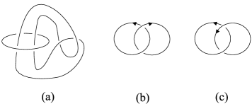
Figure 2.

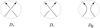
Figure 3.

4. Radon partitions in heptagonal figure-8 knot

In this section we give several lemmas necessary for the proof of Theorem 2. Throughout this section $P$ is a heptagonal figure-8 knot such that its vertices are in general position and labelled by $\{1,2,\ldots,7\}$ along an orientation. Some lemmas will be described by using tables as in Theorem 2. Note that the blanks in the tables of the following lemma and the rest of this article indicate that the values of $\epsilon$ are not decided yet.

Lemma 4.

The following implications hold for $P$.

(i) 45 56 67 123 $\pm$ $\times$ $\times$ $\quad\Longrightarrow\quad$ 56 67 71 234 $\times$ 67 71 12 345 $\mp$

(ii) 45 56 67 123 $\times$ $\times$ $\pm$ $\quad\Longrightarrow\quad$ 23 34 45 671 $\mp$ 34 45 56 712 $\times$

Proof.

Note that (i) is identical with (ii) after relabelling vertices of $P$ along the reverse orientation. Hence it suffices to prove only (i). Assume $\epsilon(123,45)=1$. Then we can choose a diagram of $P$ in which $e_{23}$ and $e_{45}$ produce a positive crossing. Figure 4-(a) depicts the diagram partially. Set $K_{+}=P$ and apply the skein relation of Conway polynomial so that

$$\nabla(K_{+})-\nabla(K_{-})=t\;\nabla(K_{0})\;,$$

where $K_{-}$ is the cycle $\langle 12\#34567\rangle$ and $K_{0}=\langle 12\#567\rangle\cup\langle 34*\rangle$ as seen in Figure 4-(b) and (c). The conditional part of (i) implies that $e_{45}$ is the only edge of $P$ piercing $\Delta_{123}$. Hence $K_{-}\sim\langle 134567\rangle$ by an isotopy in $\Delta_{123}$. Similarly $K_{0}\sim\langle 1\#567\rangle\cup\langle 34*\rangle$. Since $\langle 134567\rangle$ is a hexagon, $K_{-}$ should be trivial or trefoil by Theorem 1. Therefore, $\nabla(K_{-})=1$ or $1+t^{2}$ and because $\nabla(K_{+})=1-t^{2}$, we have

$$\nabla(K_{0})=-t\quad\mbox{or}\quad-2t\quad.$$

By Lemma 3-(iii) at least one edge of $\langle 1\#567\rangle$ penetrates $\Delta_{34*}$ in negative direction. Note that $\Delta_{34*}$ is contained in a half space $H_{123}^{-}$ with respect to the plane $H_{123}^{0}$ formed by $\{1,2,3\}$. Since $e_{1\#}$ belongs to $\Delta_{123}$ and $e_{\#5}$ belongs to another half space $H_{123}^{+}$, the two edges are excluded from candidates. Also $e_{56}$ is excluded because $\Delta_{34*}\subset\Delta_{345}$. Hence $e_{67}$ and $e_{71}$ are the only edges which may penetrate $\Delta_{34*}$. But the vertex $1$ belongs to $H_{34*}^{+}$, which implies that if $e_{71}$ penetrates $\Delta_{34*}$, then the orientation of intersection should be positive. Therefore we can conclude $\epsilon(34*,67)=-1$, and hence $\epsilon(345,67)=-1$.

Let $T_{5,123}^{\infty}$ be the set of all half infinite lines starting the vertex $5$ and passing through a point of $\Delta_{123}$. Clearly $\Delta_{234}\subset T_{5,123}^{\infty}$. Hence if we suppose $\epsilon(234,56)\neq 0$, then also $\epsilon(123,56)\neq 0$, which is contradictory to the condition of (i).

In the case that $\epsilon(123,45)=-1$ we can prove the implication in a similar way. ∎

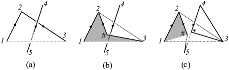
Figure 4. $K_{+}$, $K_{-}$ and $K_{0}$

Lemma 5.

$$\mbox{(i)}\quad\epsilon(123,56)=\pm 1\;\;\mbox{and}\;\;\epsilon(456,12)\neq 0\quad\Longrightarrow\quad\epsilon(456,12)=\pm 1$$

$$\mbox{(ii)}\quad\epsilon(123,56)=\pm 1\;\;\mbox{and}\;\;\epsilon(567,23)\neq 0\quad\Longrightarrow\quad\epsilon(567,23)=\pm 1$$

Proof.

Assuming $\epsilon(123,56)=1$, the conditional part of (i) can be illustrated as Figure 5-(a). From the figure we can verify (i). Similarly (ii) can be proved. ∎

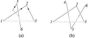
Figure 5.

Lemma 6.

(i) 45 56 67 123 $\bullet$ $\bullet$ $\quad\Longrightarrow\quad$ 67 71 12 345 $\times$ 71 12 23 456 $\bullet$ $\times$ $\times$

(ii) 45 56 67 123 $\bullet$ $\bullet$ $\quad\Longrightarrow\quad$ 12 23 34 567 $\times$ $\times$ $\bullet$ 23 34 45 671 $\times$

Proof.

Assuming $\epsilon(123,45)=1$, the conditional part of (i) can be illustrated as Figure 5-(b). The figure clearly shows that $\epsilon(345,12)=0$, $\epsilon(456,12)=0$ and $\epsilon(456,23)=0$. Note that $e_{71}$, $e_{12}$ and $e_{23}$ are the only possible edges of $P$ which may penetrate $\Delta_{456}$. Hence $\epsilon(456,71)$ should be nonzero. Otherwise, $P=\langle 1234567\rangle$ can be isotoped to the hexagon $\langle 123467\rangle$ along $\Delta_{456}$, which contradicts that $P$ is of polygon index 7 by Theorem 1. Similarly (ii) can be proved. ∎

Lemma 7.

$P$ does not allow any of two cases below:

(i) 45 56 67 123 $\times$ $\pm$ $\times$ 67 71 12 345 $\times$ $\pm$ (ii) 23 34 45 671 $\pm$ $\times$ 45 56 67 123 $\times$ $\pm$ $\times$

Proof.

Suppose that (i) is true. It suffices to consider the case that $\epsilon(123,56)=\epsilon(345,71)=1$. Apply the skein relation to the crossing between $e_{23}$ and $e_{56}$ as seen in Figure 6, so that $K_{-}\sim\langle 134567\rangle$ and $K_{0}\sim\langle 1*67\rangle\cup\langle 5\#34\rangle$. Then $\nabla(K_{0})$ should be $-t$ or $-2t$, that is, the linking number of $K_{0}$ is $-1$ or $-2$. Note that $\Delta_{5\#3}\cup\Delta_{345}$ is a Seifert surface of $\langle 5\#34\rangle$. Therefore

$$\sum_{i\in\{1*,*6,67,71\}}(\epsilon(5\#3,e_{i})+\epsilon(345,e_{i}))=-1\;\;\mbox{or}\;\;-2\;\;.$$

By our assumption $\epsilon(345,67)=0$ and $\epsilon(345,71)=1$. Clearly we know that $\epsilon(5\#3,e_{i})=0$ for $i=1*,*6$. Also $\epsilon(345,*6)$ is $0$ because $e_{*6}$ is a segment of $e_{56}$. Select the point $\#$ so that $\Delta_{5\#3}\subset\Delta_{356}$, hence $\epsilon(5\#3,67)$ is $0$. Therefore the summation should be $-1$, and $\epsilon(345,1*)=\epsilon(5\#3,71)=-1$. But the vertex $1$ belongs to $H_{5\#3}^{+}$ as seen in the figure, hence if $e_{71}$ penetrates $\Delta_{5\#3}$, then the orientation of intersection should be positive, which is a contradiction.

(ii) is derived directly from (i) by relabelling the vertices after reversing the orientation of $P$. ∎

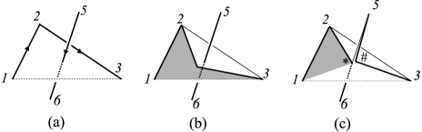
Figure 6. $K_{+}$, $K_{-}$ and $K_{0}$

Two integers $i$ and $j$ indicate the same vertex if $i\equiv j$ (mod 7). For an integer $i$, define $I(i)$ to be the number of edges of $P$ penetrating $\Delta_{i,i+1,i+2}$, that is,

$$I(i)=\sum_{j\in\{i+3,i+4,i+5\}}|\epsilon((i,i+1,i+2),(j,j+1))|\;\;.$$

Lemma 8.

There exists no integer $i$ such that $I(i)\geq 2$ and $I(i+1)\geq 2$.

Proof.

Suppose that $I(1)\geq 2$ and $I(2)\geq 2$. Then, up to the relabelling

$(1,2,3,4,5,6,7)\rightarrow(4,3,2,1,7,6,5)$

it is enough to observe the following six cases:

(i) 45 56 67 123 $\bullet$ $\bullet$ 56 67 71 234 $\bullet$ $\bullet$       (ii) 45 56 67 123 $\bullet$ $\bullet$ 56 67 71 234 $\bullet$ $\bullet$       (iii) 45 56 67 123 $\bullet$ $\bullet$ 56 67 71 234 $\bullet$ $\bullet$

(iv) 45 56 67 123 $\bullet$ $\bullet$ 56 67 71 234 $\bullet$ $\bullet$       (v) 45 56 67 123 $\bullet$ $\bullet$ 56 67 71 234 $\bullet$ $\bullet$       (vi) 45 56 67 123 $\bullet$ $\bullet$ 56 67 71 234 $\bullet$ $\bullet$

For Case (i), apply Lemma 6 to $\Delta_{123}$ and $\Delta_{234}$. Then we have

71 12 23 456 $\bullet$ $\times$ $\times$ 12 23 34 567 $\bullet$ $\times$ $\times$

But, applying Lemma 4-(i) to $\Delta_{456}$, $\epsilon(567,12)$ should be $0$, a contradiction. Also Case (iii) can be rejected in a similar way. For Case (vi) to be excluded, only Lemma 6 is enough.

For Case (ii) we may assume further that $\epsilon(123,45)=1$. Then, for $e_{71}$ to penetrate $\Delta_{234}$, the vertex $7$ should belong to $H_{123}^{-}$. This implies that the region $\Delta_{456}\cap H_{123}^{+}$ is not penetrated by any edge of $P$, and $e_{45}$ and $e_{56}$ are the only edges of $P$ penetrating $\Delta_{123}$. Hence we can isotope $P$ to $\langle 134567\rangle$ as illustrated in Figure 7, which contradicts Theorem 1. Also in Case (iv) $P$ can be isotoped to $\langle 245671\rangle$ in a similar way.

For case (v), we may suppose further that $\epsilon(123,45)=1$. Then $\Delta_{234}$ belongs to $H_{123}^{-}$. If $\epsilon(123,67)=1$, then $e_{71}$ belongs to $H_{123}^{+}$ and hence can not penetrate $\Delta_{234}$, a contradiction. Similarly if $\epsilon(123,67)=-1$, then $e_{56}$ can not penetrate $\Delta_{234}$. ∎

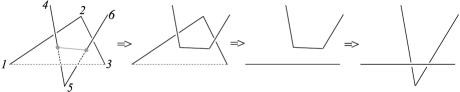
Figure 7.

Lemma 9.

There exists no pair of distinct integers $(i,j)$ such that

i+3, i+4 i+4, i+5 i+5, i+6 i, i+1, i+2 $\bullet$ $\bullet$ $\times$ j+3, j+4 j+4, j+5 j+5, j+6 j, j+1, j+2 $\times$ $\bullet$ $\bullet$

Proof.

By Lemma 8 it is enough to observe the four cases: $(i,j)=(1,3)$, $(1,4)$, $(1,5)$ and $(1,6)$. The first two cases are contradictory to Lemma 6. For the fourth case, applying Lemma 6 to $\Delta_{123}$, we have

71 12 23 456 $\bullet$ $\times$ $\times$

And apply Lemma 4 to $\Delta_{456}$, to have $\epsilon(671,23)\neq 0$, a contradiction.

Lastly suppose $(i,j)=(1,5)$. Then, we can observe which edges penetrate $\Delta_{671}$ and $\Delta_{712}$ as follows:

	45	56	67
123	$\bullet$	$\bullet$	$\times$
	12	23	34
567	$\times$	$\bullet$	$\bullet$

Lemma 6

$\Longrightarrow$

	56	67	71
234	$\times$	$\times$	$\bullet$
	71	12	23
456	$\bullet$	$\times$	$\times$

Lemma 4

$\Longrightarrow$

	23	34	45
671	$\bullet$
	34	45	56
712			$\bullet$

Lemma 8
$\Longrightarrow$
$(i,j)=(1,5)$

	23	34	45
671	$\bullet$	$\times$	$\times$
	34	45	56
712	$\times$	$\times$	$\bullet$

We may assume $\epsilon(123,45)=1$. Then clearly $\epsilon(123,56)=-1$, and by Lemma 4 $\epsilon(671,23)=-1$. Now we apply the skein relation to $e_{23}\cup e_{67}$ as seen in Figure 8 so that $K_{-}=P$, $K_{0}\sim\langle 6\#345\rangle\cup\langle 2*1\rangle$ and $\Delta_{2*1}\subset\Delta_{123}$. Then immediately it is observed that

$$\epsilon(2*1,6\#)=\epsilon(2*1,\#3)=\epsilon(2*1,34)=0$$

Recall $\epsilon(123,56)=-1$, which implies that if $\epsilon(2*1,56)\neq 0$, then the value should be negative. Therefore, considering $\nabla(K_{0})=t$ or $2t$, it should hold that

$$\epsilon(2*1,45)=1,\quad\epsilon(2*1,56)=0$$

and $e_{56}$ penetrates $\Delta_{*31}=\Delta_{123}-\Delta_{2*1}$. Since $\Delta_{*31}\subset H_{671}^{-}$, the vertex $5$ belongs to $H_{671}^{-}$. Hence $e_{56}\subset H_{671}^{-}$, which is contradictory to $\epsilon(712,56)\neq 0$ because $\Delta_{712}$ belongs to the other half space $H_{671}^{+}$. ∎

Figure 8. $K_{-}$, $K_{+}$ and $K_{0}$

Lemma 10.

(i) For every $i$, $I(i)\geq 1$.

(ii) There exists an integer $i$ such that $I(i)\geq 2$.

(iii) For every $i$, $I(i)<3$.

(iv) If $I(i)=2$ for some $i$, then $e_{i+4,i+5}$ should penetrate $\Delta_{i,i+1,i+2}$.

Proof of (i)..

Suppose $I(1)=0$, that is, $\Delta_{123}$ is not penetrated by any edge of $P$. Then we can isotope $P$ along $\Delta_{123}$, so that $P\sim\langle 134567\rangle$. By Theorem 1, the hexagon $\langle 134567\rangle$ is trivial or trefoil, a contradiction. ∎

Proof of (ii)..

Suppose $I(i)=1$ for every $i$. Then, among $e_{45}$, $e_{56}$ and $e_{67}$, only one edge penetrates $\Delta_{123}$. Firstly assume that $e_{45}$ does. Then, applying Lemma 4 repeatedly, we have a sequence of implications:

45 56 67 123 $\bullet$ $\times$ $\times$ $\Longrightarrow$ 67 71 12 345 $\bullet$ $\times$ $\times$ $\Longrightarrow$ 12 23 34 567 $\bullet$ $\times$ $\times$ $\Longrightarrow$

34 45 56 712 $\bullet$ $\times$ $\times$ $\Longrightarrow$ 56 67 71 234 $\bullet$ $\times$ $\times$

But, by Lemma 4 again, the first and last tables are contradictory to each other. The case that $e_{67}$ penetrates the triangle is rejected in a similar way.

Now it can be assumed that every $\Delta_{i,i+1,i+2}$ is penetrated only by $e_{i+4,i+5}$. Then, applying Lemma 5 repeatedly, we have that

45 56 67 123 $\times$ $\pm$ $\times$ and 67 71 12 345 $\times$ $\pm$ $\times$ ,

which is contradictory to Lemma 7. ∎

Proof of (iii)..

Suppose $I(1)=3$. Then we have two implications as follows:

	45	56	67
123	$\bullet$	$\bullet$

Lemma 6

$\Longrightarrow$

	71	12	23
456	$\bullet$	$\times$	$\times$

Lemma 4

$\Longrightarrow$

	23	34	45
671	$\bullet$

	45	56	67
123		$\bullet$	$\bullet$

Lemma 6

$\Longrightarrow$

	23	34	45
671	$\times$

But these are contradictory to each other. ∎

Proof of (iv)..

Suppose that $\Delta_{123}$ satisfies the following:

45 56 67 123 $\bullet$ $\times$ $\bullet$

Then it is enough to observe two cases $(\epsilon(123,45),\epsilon(123,67))=(1,-1)$ and $(1,1)$. These cases are depicted as in Figure 9-(a) and (b) respectively. In the first case $5$ and $6$ are the only vertices which belong to $H_{123}^{+}$. Therefore P can be isotoped to $\langle 1234*\#7\rangle$ along the tetragon formed by $\{*,5,6,\#\}$. And lift $e_{*\#}$ slightly into $H_{123}^{-}$, then we have $I(1)=0$ for the resulting heptagon, a contradiction.

For the second case we observe which edges penetrate $\Delta_{234}$. Note that $\Delta_{234}\subset T_{5,123}^{\infty}$. Hence if a line starting at the vertex $5$ penetrates $\Delta_{234}$, then it also penetrates $\Delta_{123}$. This implies $\epsilon(234,56)=0$. Also $\epsilon(234,71)=0$, because $e_{71}$ belongs to $H_{123}^{+}$ but $\Delta_{234}$ belongs to the other half space $H_{123}^{-}$. Therefore $e_{67}$ is the only edge of $P$ penetrating $\Delta_{234}$. Furthermore the orientation of intersection should be positive. This can be seen easily from Figure 9-(c). Let $N$ be a plane in $\mathbb{R}^{3}$ orthogonal to $\overrightarrow{23}$. And let $\pi:\mathbb{R}^{3}\equiv N\times\mathbb{R}\rightarrow N$ be the orthogonal projection onto $N$ such that the vertex $3$ is above the vertex $2$ with respect to the $\mathbb{R}$-coordinate. Figure 9-(c) depicts the image of $H_{123}^{0}\cup H_{234}^{0}$ under $\pi$. Suppose $\epsilon(234,67)=-1$. Since $\epsilon(123,67)=1$, the vertex 6 should belong to $H_{123}^{-}\cap H_{234}^{+}$ which corresponds to the shaded region in the figure. Then, as seen in the figure, it is impossible that $e_{67}$ penetrates both $\Delta_{123}$ and $\Delta_{234}$.

In a similar way $e_{45}$ should be the only edge of $P$ penetrating $\Delta_{712}$ and the orientation of intersection is positive. To summarize, we have

56 67 71 234 $\times$ $+$ $\times$ and 34 45 56 712 $\times$ $+$ $\times$

This contradicts Lemma 7. ∎

Figure 9.

5. Proof of theorem 2

We prove the “only if” part of Theorem 2 by filling in the table of penetrations in $P$. By Lemma 10 it can be assumed that

45 56 67 123 $\bullet$ $\bullet$ $\times$

Applying Lemma 6 to $\Delta_{123}$ and Lemma 4 to $\Delta_{456}$, we have the initial status $S_{0}$ as shown in Table 1. Considering Lemma 9, we know that the row of $567$ should be filled by $(\times,\bullet,\times)$ or $(\times,\times,\bullet)$. The second is excluded by Lemma 4. Lemma 10-(iv) guarantees $\epsilon(671,45)=0$. Hence the status $S^{\prime}_{0}$ is derived. Observe how the row of $712$ can be filled. $I(7)$ should be $1$ or $2$ by Lemma 10-(i) and (iii). In fact $I(7)$ should be 1 by Lemma 8. And $(\bullet,\times,\times)$ and $(\times,\times,\bullet)$ are disallowed by Lemma 4, hence $S^{\prime\prime}_{0}$ is derived.

In a similar way we know that $234$ should have $(\bullet,\times,\times)$ or $(\times,\bullet,\times)$. Hence $S^{\prime\prime}_{0}$ can proceed to the status $S_{1}$ or $S_{2}$.

Case 1: the row of $234$ is filled with $(\bullet,\times,\times)$. Observe $345$ in $S_{1}$. Apply Lemma 4 to $\Delta_{234}$. Then $\epsilon(345,67)=0$, and $\epsilon(345,71)\neq 0$. Therefore we obtain $S_{1}^{\prime}$. Finally, let $S_{1-1}^{\prime}$ (resp. $S_{1-2}^{\prime}$) be the status obtained from $S_{1}^{\prime}$ by setting $\epsilon(671,34)$ to be zero (resp. nonzero).

Note that if the table is completely filled with “$\bullet$” and“$\times$”, then the orientation of intersection is automatically determined. See $S_{1-1}^{\prime}$. Since $123$ has $(\bullet,\bullet,\times)$, the possible orientation is $(+,-,\times)$ or $(-,+,\times)$. Assume the former. Applying Lemma 4 to $\Delta_{671}$, we know $\epsilon(671,23)=-1$. Also applying the lemma to $\Delta_{456}$ and $\Delta_{234}$, we have $\epsilon(456,71)=1$ and $\epsilon(234,56)=-1$. Furthermore, from the assumption $\epsilon(123,56)=-1$, it is derived that $\epsilon(567,23)=-1$ and $\epsilon(345,71)=1$ by Lemmas 5 and 7 respectively. Similarly $\epsilon(712,45)=1$. Therefore $S_{1-1}^{\prime}$ is identical with RS-I.

For $S_{1-2}^{\prime}$, first determine the orientations in the second column following the method used above. Then, under the assumption $\epsilon(123,56)=-1$, it should hold that $\epsilon(671,34)=1$. This implies $\epsilon(671,23)=-1$, from which the orientations in the first column can be determined. In this way we can verify that $S_{1-2}^{\prime}$ is identical with RS-II.

Case 2: the row of $234$ is filled with $(\times,\bullet,\times)$. If $671$ has $(\bullet,\bullet,\times)$ in $S_{2}$, then $234$ should have $(\bullet,\times,\times)$ by Lemma 6, a contradiction. Therefore $S_{2}$ proceeds only to $S_{2}^{\prime}$. Suppose that $345$ can be filled with $(\bullet,\times,\times)$. Then also we can derive a contradiction by applying Lemma 4 to $\Delta_{345}$. Hence, in $S_{2}^{\prime}$, $345$ should have $(\bullet,\bullet,\times)$ or $(\times,\bullet,\times)$. In the former case we have $S_{2-1}^{\prime}$ which becomes RS-II after relabelling vertices by the cyclic permutation sending $(3,4,5)$ to $(1,2,3)$. In the latter we have $S_{2-2}^{\prime}$ which is RS-III.

	45	56	67
123	$\bullet$	$\bullet$	$\times$
	56	67	71
234
	67	71	12
345			$\times$
	71	12	23
456	$\bullet$	$\times$	$\times$
	12	23	34
567	$\times$
	23	34	45
671	$\bullet$
	34	45	56
712
$S_{0}$

$\Rightarrow$ 45 56 67 123 $\bullet$ $\bullet$ $\times$ 56 67 71 234 67 71 12 345 $\times$ 71 12 23 456 $\bullet$ $\times$ $\times$ 12 23 34 567 $\times$ $\bullet$ $\times$ 23 34 45 671 $\bullet$ $\times$ 34 45 56 712 $S^{\prime}_{0}$ $\Rightarrow$ 45 56 67 123 $\bullet$ $\bullet$ $\times$ 56 67 71 234 67 71 12 345 $\times$ 71 12 23 456 $\bullet$ $\times$ $\times$ 12 23 34 567 $\times$ $\bullet$ $\times$ 23 34 45 671 $\bullet$ $\times$ 34 45 56 712 $\times$ $\bullet$ $\times$ $S^{\prime\prime}_{0}$

	45	56	67
123	$\bullet$	$\bullet$	$\times$
	56	67	71
234	$\bullet$	$\times$	$\times$
	67	71	12
345			$\times$
	71	12	23
456	$\bullet$	$\times$	$\times$
	12	23	34
567	$\times$	$\bullet$	$\times$
	23	34	45
671	$\bullet$		$\times$
	34	45	56
712	$\times$	$\bullet$	$\times$
$S_{1}$

$\Rightarrow$ 45 56 67 123 $\bullet$ $\bullet$ $\times$ 56 67 71 234 $\bullet$ $\times$ $\times$ 67 71 12 345 $\times$ $\bullet$ $\times$ 71 12 23 456 $\bullet$ $\times$ $\times$ 12 23 34 567 $\times$ $\bullet$ $\times$ 23 34 45 671 $\bullet$ $\times$ 34 45 56 712 $\times$ $\bullet$ $\times$ $S^{\prime}_{1}$    45 56 67 123 $\bullet$ $\bullet$ $\times$ 56 67 71 234 $\bullet$ $\times$ $\times$ 67 71 12 345 $\times$ $\bullet$ $\times$ 71 12 23 456 $\bullet$ $\times$ $\times$ 12 23 34 567 $\times$ $\bullet$ $\times$ 23 34 45 671 $\bullet$ $\times$ $\times$ 34 45 56 712 $\times$ $\bullet$ $\times$ $S^{\prime}_{1-1}$    45 56 67 123 $\bullet$ $\bullet$ $\times$ 56 67 71 234 $\bullet$ $\times$ $\times$ 67 71 12 345 $\times$ $\bullet$ $\times$ 71 12 23 456 $\bullet$ $\times$ $\times$ 12 23 34 567 $\times$ $\bullet$ $\times$ 23 34 45 671 $\bullet$ $\bullet$ $\times$ 34 45 56 712 $\times$ $\bullet$ $\times$ $S^{\prime}_{1-2}$

	45	56	67
123	$\bullet$	$\bullet$	$\times$
	56	67	71
234	$\times$	$\bullet$	$\times$
	67	71	12
345			$\times$
	71	12	23
456	$\bullet$	$\times$	$\times$
	12	23	34
567	$\times$	$\bullet$	$\times$
	23	34	45
671	$\bullet$		$\times$
	34	45	56
712	$\times$	$\bullet$	$\times$
$S_{2}$

$\Rightarrow$ 45 56 67 123 $\bullet$ $\bullet$ $\times$ 56 67 71 234 $\times$ $\bullet$ $\times$ 67 71 12 345 $\times$ 71 12 23 456 $\bullet$ $\times$ $\times$ 12 23 34 567 $\times$ $\bullet$ $\times$ 23 34 45 671 $\bullet$ $\times$ $\times$ 34 45 56 712 $\times$ $\bullet$ $\times$ $S_{2}^{\prime}$    45 56 67 123 $\bullet$ $\bullet$ $\times$ 56 67 71 234 $\times$ $\bullet$ $\times$ 67 71 12 345 $\bullet$ $\bullet$ $\times$ 71 12 23 456 $\bullet$ $\times$ $\times$ 12 23 34 567 $\times$ $\bullet$ $\times$ 23 34 45 671 $\bullet$ $\times$ $\times$ 34 45 56 712 $\times$ $\bullet$ $\times$ $S_{2-1}^{\prime}$    45 56 67 123 $\bullet$ $\bullet$ $\times$ 56 67 71 234 $\times$ $\bullet$ $\times$ 67 71 12 345 $\times$ $\bullet$ $\times$ 71 12 23 456 $\bullet$ $\times$ $\times$ 12 23 34 567 $\times$ $\bullet$ $\times$ 23 34 45 671 $\bullet$ $\times$ $\times$ 34 45 56 712 $\times$ $\bullet$ $\times$ $S_{2-2}^{\prime}$   

Table 1.

Now we prove the “if” part of the theorem. Suppose $P$ is a heptagonal knot satisfying RS-I, II or III. Let $N$ be a plane orthogonal to $\overrightarrow{23}$, and $\pi:\mathbb{R}^{3}\equiv N\times\mathbb{R}\rightarrow N$ be the orthogonal projection onto $N$ such that the vertex $3$ is above the vertex $2$ with respect to the $\mathbb{R}$-coordinate. We will construct a diagram of $P$ from the projected image $\pi(P)$. Without loss of generality it can be assumed that $\epsilon(123,45)=1$ and $\epsilon(123,56)=-1$. Then, since the vertex $3$ is above $2$, the edge $e_{45}$ should pass above $e_{12}$ as illustrated in Figure 10.

Suppose $P$ corresponds to RS-I. Then similarly $e_{56}$ passes above $e_{12}$ and below $e_{34}$. Note that if $7$ belongs to $H_{123}^{-}$, then $e_{23}$ can not penetrate $\Delta_{671}$. Hence $7\in H_{123}^{+}$. Since $\epsilon(567,23)=-1$, the point $\pi(e_{23})$ should belong to $\pi(\Delta_{567})$. Therefore the point $\pi(7)$ belongs to the shaded region shown in Figure 11-(a). From this we know that $\pi(7)\notin\pi(\Delta_{456})$. And clearly $\pi(1)\notin\pi(\Delta_{456})$. Hence, for $\epsilon(456,71)$ to be nonzero, $\pi(e_{71})$ should intersect both $\pi(e_{45})$ and $\pi(e_{56})$. In fact $e_{71}$ passes above $e_{45}$ because $\epsilon(712,45)=1$ and $e_{45}$ passes above $e_{12}$. Therefore, since $\epsilon(456,71)$ is nonzero, $e_{71}$ should pass below $e_{56}$. The resulting diagram represents figure-8 as seen in Figure 11-(b). Also when $P$ corresponds to RS-II, we can obtain a diagram of figure-8 in the same way.

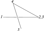
Figure 10.

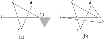
Figure 11.

Suppose $P$ corresponds to RS-III. Again assume $\epsilon(123,45)=1$ and $\epsilon(123,56)=-1$. Then also in this case we have that $6\in H_{123}^{-}$ and $7\in H_{123}^{+}$. Especially it should hold that $6\in H_{234}^{+}$ and $7\in H_{234}^{-}$, because $\epsilon(234,67)=-1$. Hence the vertex $6$ is projected into the shaded region in the top-left of Figure 12-(a) and the vertex $7$ into the bottom-right. Now we observe two possible cases according to the position of $\pi(6)$ with respect to $\pi(e_{45})$ as shown in Figure 12-(b) and (c). Again since $\epsilon(234,67)$ is nonzero, $e_{67}$ should pass below $e_{34}$ in both diagrams. As discussed in the case of RS-I, from $\epsilon(456,71)=1$, we know that $e_{71}$ passes above $e_{45}$ and below $e_{56}$. Then the resulting diagram in (b) represents figure-8. In (c), for $e_{71}$ to pass above $e_{45}$ and below $e_{56}$, the two vertices $6$ and $7$ should belong to $H_{145}^{-}$, which implies that $e_{67}$ passes above $e_{45}$. Therefore also the resulting diagram in (c) represents figure-8.

Figure 12.

References

- [1] J. L. Ramírez Alfonsín, Spatial graphs and oriented matroids: the trefoil, Discrete Comput. Geom. 22 (1999), 149–158.
- [2] A. Björner, M. Las Vergnas, B. Sturmfels, N. White and G. Ziegler, Oriented matroids, Encyclopedia of Mathematics and its Applications, 46. Cambridge University Press, Cambridge, 1993.
- [3] J. A. Calvo, Geometric Knot Theory, Ph.D. Thesis, Univ. Calif. Santa Barbara, 1998.
- [4] J. H. Conway and McA. G. Gordon, Knots and links in spatial graphs, J. Graph Theory 7 (1983), no. 4, 445–453.
- [5] L. Finschi, A Graph Theoretical Approach for Reconstruction and Generation of Oriented Matroids, Dissertation, Swiss Federal Institute of Technology (ETH) Zurich (2001)
- [6] Homepage of oriented matroid, http://www.om.math.ethz.ch/
- [7] E. Furstenberg, J. Li and J. Schneider, Stick knots, Chaos, Solitons and Fractals 9 (1998) 561–568.
- [8] Y. Huh and C. B. Jeon, Knots and links in linear embeddings of , J. Korean Math. Soc. 44 (2007), 661–671.
- [9] G. T. Jin, Polygonal indices and superbridges indices of torus knots and links, J. Knot Theory Ramif. 6 (1997) 281–289.
- [10] L. H. Kauffman, On knots, Annals of Mathematics Studies, 115. Princeton University Press, Princeton, NJ, 1987.
- [11] K. Murasugi, Knot theory and its applications, Translated from the 1993 Japanese original by Bohdan Kurpita. Birkhauser Boston, Inc., Boston, MA, 1996.
- [12] L. Mccabe, An upper bound on edge numbers of 2-bridge knots and links, J. Knot Theory Ramif. 7 (1998) 797–805.
- [13] S. Negami, Ramsey theorems for knots, links and spatial graphs, Trans. Amer. Math. Soc. 324 (1991), no. 2, 527–541.
- [14] R. Randell, An elementary invariant of knots, J. Knot Theory Ramifications 3 (1994), 279–286.
- [15] R. Randell, Invariants of piecewise-linear knots, Knot theory (Warsaw, 1995), 307–319, Banach Center Publ., 42, Polish Acad. Sci., Warsaw, 1998.
- [16] D. Rolfsen, Knots and links, Mathematics Lecture Series, No. 7. Publish or Perish, Inc., Berkeley, Calif., 1976.