C2D Spitzer-IRS spectra of disks around T Tauri stars
V. Spectral decomposition

Abstract

Context. Dust particles evolve in size and lattice structure in protoplanetary disks, due to coagulation, fragmentation and crystallization, and are radially and vertically mixed in disks due to turbulent diffusion and wind/radiation pressure forces.

Aims. This paper aims at determining the mineralogical composition and size distribution of the dust grains in planet forming regions of disks around a statistical sample of 58 T Tauri stars observed with Spitzer/IRS as part of the Cores to Disks (c2d) Legacy Program.

Methods. We present a spectral decomposition model, named “B2C”, that reproduces the IRS spectra over the full spectral range (5–35 $\mu$m). The model assumes two dust populations: a warm component responsible for the 10 $\mu$m emission arising from the disk inner regions ($\lesssim$ 1 AU) and a colder component responsible for the 20–30 $\mu$m emission, arising from more distant regions ($\lesssim$ 10 AU). The fitting strategy relies on a random exploration of parameter space coupled with a Bayesian inference method.

Results. We show evidence for a significant size distribution flattening in the atmospheres of disks compared to the typical MRN distribution, providing an explanation for the usual flat, boxy $10\,\mu$m feature profile generally observed in T Tauri star spectra. We reexamine the crystallinity paradox, observationally identified by Olofsson et al. (2009), and we find a simultaneous enrichment of the crystallinity in both the warm and cold regions, while grain sizes in both components are uncorrelated. We show that flat disks tend to have larger grains than flared disk. Finally our modeling results do not show evidence for any correlations between the crystallinity and either the star spectral type, or the X-ray luminosity (for a subset of the sample).

Conclusions. The size distribution flattening may suggests that grain coagulation is a slightly more effective process than fragmentation (helped by turbulent diffusion) in disk atmospheres, and that this imbalance may last over most of the TTauri phase. This result may also point toward small grain depletion via strong stellar winds or radiation pressure in the upper layers of disk. The non negligible cold crystallinity fractions suggests efficient radial mixing processes in order to distribute crystalline grains at large distances from the central object, along with possible nebular shocks in outer regions of disks that can thermally anneal amorphous grains.

1 Introduction

The mid-infrared spectral regime probes the warm dust grains located in the planet forming region (typically 1–10 AU for a classical T Tauri disk). At these wavelengths, the young disks are optically opaque to the stellar light, and the thermal emission arises from the disk surface, well above the disk midplane. Single-aperture imaging of disks in the mid-IR suffers from both a relatively low spatial resolution compared to optical/near-IR telescopes, and from poorly extended emission zones. On the other hand, silicates have features due to stretching and bending resonance modes which make spectroscopy at mid-IR wavelengths of very high interest and feasible with current instrumentation. Silicates are indeed the most abundant sort of solids in disks, and therefore constitute a very important ingredient in any planet formation theory.

The dust grains that are originally incorporated into protoplanetary circumstellar disks are essentially of interstellar nature. They are thought to be particles much smaller than $1\,\mu$m, and mostly composed of silicates or organic refractories. Kemper et al. (2005) placed an upper limit of 2.2% on the amount of crystalline silicates in the interstellar medium (hereafter ISM), which suggests an amorphous lattice structure for the pristine silicates in forming protoplanetary disks. In the very early stages of the disk evolution, the tiny dust grains are so coupled with the gas that grain-grain collisions occur at sufficiently low relative velocity to allow the grains to coagulate and grow. This results in fractal aggregates that will tend to settle toward the disk midplane as their mass increases. From simple theoretical arguments, considering only the gravitational and drag forces on the grains in a laminar disk, one can show that $\mu$m-sized grains at 1 AU should settle in the midplane in less than $10^{5}$ years in a classical T Tauri disk (Weidenschilling 1980). In fact, the grains are expected to settle even faster as their mass increases in the course of their journey to the disk midplane. Because the T Tauri disks are a few million years old, this would suggest that the inner disk upper layers should be devoided of $\mu$m-sized or larger grains in the absence of turbulence and grain fragmentation. This is a prediction that can be tested observationnaly, especially in the infrared where spectroscopic signatures of silicate grains are present.

The Spitzer Space Telescope, launched in August 2003, had a sensitivity that surpassed previous mid-IR space missions by orders of magnitudes until the cryogenic mission ended in May 2009. As part of the “Core to Disks” (c2d) Legacy survey (Evans et al., 2003), more than a hundred T Tauri stars were spectroscopically observed, to confirm or invalidate some of the predictions concerning dust processing and grain dynamics in protoplanetary disks. In Kessler-Silacci et al. (2006, 2007), and Olofsson et al. (2009), we showed that most of the objects display silicate emission features arising from within 10 AU from the star. This allowed both a classical study of grain coagulation and a comprehensive statistical analysis of dust crystallization in planet forming regions of disks around young solar analogs.

In Olofsson et al. (2009), we showed that not only the warm amorphous silicates had grown, but so had the colder crystalline silicates as probed by their $23\,\mu$m emission feature. In fact, the emission features in IRS spectra are very much dominated by micron-sized grains in the upper layers of disks, pointing toward vertical (turbulent?) mixing of the dust grains to compensate for gravitational settling, together with grain-grain destructive fragmentation in the innermost regions of most protoplanetary disks to compensate for grain growth. This equilibrium seems to last over several millions of years and be to independent of the specific star forming region (Oliveira et al. 2010). Winds and/or radiation pressure, in complement to these processes, can act to remove a fraction of the submicron-sized grains from disk atmospheres, and may thus contribute to the transport of crystalline silicate grains toward the outermost disk regions (see discussion in Olofsson et al. 2009).

Crystalline silicates appear to be very frequent in disks around T Tauri disks and in regions much colder than their presumed formation regions, suggesting efficient outward radial transport mechanisms in disks (Bouwman et al. 2008; Olofsson et al. 2009; Watson et al. 2009a). Therefore, the determination of the composition and size distribution of the dust grains in circumstellar disks is one of the keys in understanding the first steps of planet formation as it can trace the dust fluxes in planet-forming disks. Detailed modeling of the $10\,\mu$m silicate emission feature has already been performed for HAEBE disks by Bouwman et al. (2001) and van Boekel et al. (2005). Mineralogical studies of dust in disks around very low mass stars and brown dwarfs were also led by Apai et al. (2005), Riaz (2009), Merín et al. (2007) and Bouy et al. (2008). The two last studies introduced a novel method to fit the spectra over the entire IRS spectral range, which allows to decompose the spectra into two main contributions at different temperatures. This in turn allowed to compare the degrees of crystallinity and the grain sizes in two different disk regions. The latter compositional fitting approach is further supported by the analysis by Olofsson et al. (2009) who showed that the energy and frequencies at which crystalline silicate features are seen at wavelengths larger than $20\,\mu$m are largely uncorrelated to the amorphous $10\,\mu$m feature observational properties.

We present in this paper an improved version of the compositional fitting method used in Merín et al. (2007) and Bouy et al. (2008). We apply the model to a subsample (58 stars) of high SNR spectra presented in Olofsson et al. (2009) to derive the dust content in disks about young solar analogs. The method relies on the fact that the IRS spectral range is sufficiently broad so that the regions probed at around $10\,\mu$m and between $20$ and $30\,\mu$m do overlap only partially. This is illustrated for instance in Kessler-Silacci et al. (2006) who show that for a typical T Tauri star, a factor of 2 increase in wavelength ($10\,\mu$m $\rightarrow$ $20\,\mu$m), translates into a factor of 10 ($1\,$AU $\rightarrow$ $10\,$AU) into the regions from which most of the observed emission arises. An additional goal of our model is therefore to search for differential effects in crystallinity and grain sizes between the warm and slightly cooler disks regions which may be indicative of radial and/or vertical dependent chemical composition and grain size, due for instance to differential grain evolution and/or grain transport.

We develop in Sec. 2 our procedure to model IRS spectra of Class II objects, and present the tests for robustness of this procedure in Appendix A. The results for 58 objects are presented in Sec. 3, and they are discussed in terms of dust coagulation and dust crystallization in Sec. 4. Sec. 5 summarizes the implications of our results on disks dynamics at this stage of evolution and critically discuss the use of the shape and strength of the amorphous $10\,\mu$m silicate feature as a grain proxy.

2 Spectral decomposition with the B2C method

We elaborate in this section a modeling procedure whose goal is to reproduce the observed IRS spectra, from about $5$ to $35\,\mu$m, in order to infer the composition and size of the emitting dust grains. This is achevied by using two dust grain populations at two different temperatures. We will refer to these two populations as two different “components”. The first component aims at reproducing the features at around $10\,\mu$m, its temperature is generally around $T_{\mathrm{w}}\sim 300$ K (warm component hereafter). The second component aims at reproducing the residuals, over the full spectral range and its temperature is colder, $T_{\mathrm{c}}\sim 100$ K (cold component hereafter). Each of these two components is described by several grain compositions, including amorphous and crystalline silicates, and sizes as detailed below. Bayesian inference is used to best fit the IRS spectra and to derive uncertainties on the parameters, hence the name of the procedure, “B2C”, which stands for Bayesian inference with 2 Components.

2.1 Theoretical opacities and grain sizes

To reproduce the observed spectra, we consider five different dust species. The amorphous species include silicates of olivine stoichiometry (glassy MgFeSiO₄, density of 3.71 g.cm^-3, optical indexes from Dorschner et al. 1995), silicates of pyroxene stoichiometry (glassy MgFeSiO₆, density of 3.2 g.cm^-3, Dorschner et al. 1995), and silica (amorphous quartz, density of 3.33 g.cm^-3, Henning & Mutschke 1997). For the Mg-rich (see Olofsson et al. 2009) crystalline species, we consider enstatite (MgSiO₃, density of 2.8 g.cm^-3, Jaeger et al. 1998) and forsterite (Mg₂SiO₄, density of 2.6 g.cm^-3, Servoin & Piriou 1973).

Figure 1: Blowup of the opacities (in units of cm².g^-1) used to model the IRS spectra. The solid line is for 0.1 $\mu$m grains, dashed line for 1.5 $\mu$m grains and dotted line for 6.0 $\mu$m grains.

Following previous papers (e.g. Bouwman et al. 2001, 2008, Juhász et al. 2009), the theoretical opacities $\kappa_{\lambda}$ of amorphous species are computed assuming homogeneous sphere (Mie theory), while the DHS theory (Distribution of Hollow Spheres, Min et al. 2005) is employed for the crystalline silicates in order to simulate irregularly-shaped dust particles. To limit the number of free parameters in the model, we consider three spectroscopically representative grain sizes radii, which are $0.1\,\mu$m, $1.5\,\mu$m and $6.0\,\mu$m. These three grain sizes are supposed to best mimic the behaviour of very small grains, intermediate-sized grains and large grains (e.g. Bouwman et al. 2001, 2008). We limit ourselves to the two smallest sizes, 0.1 and 1.5 $\mu$m, for the crystalline species. The first reason for this choice is that large crystalline grains present a high degeneracy with large amorphous grains, as 6.0 $\mu$m-sized grains are mostly featureless. Therefore large crystals can be used by the procedure instead of large amorphous grains, thereby introducing a bias toward high crystallinity fractions. The second reason is that, according to crystallisation models (e.g. Gail 2004), one does not expect to produce such large pure crystals via thermal annealing. Grains more likely grow via collisional aggregation of both small crystalline and amorphous material (e.g. Min et al. 2008). Following these two considerations, we decided not to include 6.0 $\mu$m-sized crystals. This choice is in line with previous works from Sargent et al. (2009) or Riaz (2009). The fifteen opacity curves (5 grain compositions, 3 grain sizes) used in this paper are displayed in Fig. 1, including 6.0 $\mu$m-sized crystals to show the degeneracy with large amorphous grains.

2.2 The B2C model

The B2C model elaborated in this paper assumes that the IRS spectrum can be fitted by considering a continuum emission, and two main components, a warm and a cold one, essentially responsible for the 10$\,\mu$m and 20–30 $\mu$m emissions, respectively. The two component approach is supported by the work of Olofsson et al. (2009) who show that disks usually have inhomogeneous compositions with respect to the dust temperature (crystalline features being more frequently detected at long than at short wavelengths, the so-called crystallinity paradox), and that the emission features at around 10$\,\mu$m are essentially uncorrelated with those appearing at wavelengths larger than 20$\,\mu$m. This approach is also supported by the T Tauri model described in Kessler-Silacci et al. (2006) where they show that the emission at 10 $\mu$m is arising from regions within $\sim$ 1 AU while the flux at 20 $\mu$m is arising from within $\sim$ 10 AU. Furthermore, we first used the simpliest solution, with only one component, without successful results. Any compositional method that aims at fitting IRS spectra over the full spectral range should therefore be able to handle inhomogeneous disk compositions. The two component approach developed in this paper is a simple attempt to go in that direction. This modeling strategy has already proven sufficient to provide adequate fits to IRS spectra, from 5 to 35$\,\mu$m (Merín et al. 2007; Bouy et al. 2008). In this paper, we improve both the model and the fitting strategy originally developed in Merín et al. (2007) and Bouy et al. (2008) in order to apply the decompositional method to a large number of objects.

The first step of the modeling approach is the estimate of the continuum to be subtracted to the observed IRS spectrum before performing a compositional fit. This could be done using a radiative transfer code (e.g. Merín et al. 2007; Bouy et al. 2008), but given the number of objects (58) to be analyzed, and given the objectives of the paper which is oriented toward searching for trends thanks to the analysis of a large sample, obtaining a satisfying model for every object is not a manageable task. We instead adopt a continuum built by using a power-law ($\lambda^{\alpha}$) plus a black-body at temperature $T_{\rm cont}$, to make our problem more tractable:

$$F_{\mathrm{\nu,cont}}=K_{\rm pl}\lambda^{\alpha}+K_{\rm bb}B_{\nu}(T_{\rm cont})$$ (1)

where $K_{\rm pl}$ and $K_{\rm bb}$ are two positive constants. The power law index, $\alpha$, is determined independently from the compositional procedure. It represents the mid-IR tail of the emission from both the star itself and from the inner rim of the disk. Its value is estimated by fitting the IRS spectrum from its shortest wavelength (about 5$\,\mu$m) up to blue foot of the 10 $\mu$m amorphous silicate feature. The black-body is aimed at contributing at wavelengths larger than $20\,\mu$m and $T_{\rm cont}$ therefore constrained to be less than 150 K. A typical value for the temperature $T_{\rm cont}$ is found to be about 110 K.

In our fitting approach, only two free parameters characterize the continuum: the black-body temperature $T_{\rm cont}$ and a normalization offset $O_{\nu_{2}}$ at $\lambda_{2}=c/\nu_{2}\sim 13.5\,\mu$m. The implementation of a variable offset comes from the fact that the 10 and 18$\,\mu$m amorphous features partly overlap at $\lambda\sim$13–15 $\mu$m (Fig. 1), and any realistic continuum should therefore pass below the observed flux at these wavelengths. For a given set of $\alpha$, $T_{\rm cont}$ and offset value $O_{\nu_{2}}$, the synthetic continuum is obtained by solving the following two-equation system with respect to the normalization coefficients $K_{\rm pl}$ and $K_{\rm bb}$:

$$\left\{\begin{array}[]{ccl}K_{\rm pl}\times\lambda_{1}^{\alpha}+K_{\rm bb}\times B_{\nu_{1}}(T_{\mathrm{cont}})&=&F_{\mathrm{\nu_{1},\mathrm{obs}}}\\ K_{\rm pl}\times\lambda_{2}^{\alpha}+K_{\rm bb}\times B_{\nu_{2}}(T_{\mathrm{cont}})&=&F_{\mathrm{\nu_{2},\mathrm{obs}}}\times(1-O_{\nu_{2}})\end{array}\right.$$ (4)

where $F_{\nu,\mathrm{obs}}$ is the observed spectrum, in units of Jansky. The constraints on the normalization coefficients ($K_{\rm pl}>0$ and $K_{\rm bb}\geq 0$) imply that for some objects, the best continua require $K_{\rm bb}=0$, corresponding to continua described by a pure power-law. The normalization wavelengths are chosen to bracket the amorphous 10$\,\mu$m silicate feature, with $\lambda_{1}=c/\nu_{1}\sim 7.5$ $\mu$m, and $\lambda_{2}=c/\nu_{2}\sim 13.5$ $\mu$m.

The fit to the continuum-subtracted IRS spectrum is performed in two steps. First, a fit to the 10 $\mu$m feature is obtained between $\lambda_{1}$ and $\lambda_{2}$ (warm component), then a second fit to the residual spectrum is obtained for wavelengths between $\lambda_{1}$ and $\lambda_{3}\sim$35 $\mu$m (cold component). The continuum-substracted IRS spectrum ($F_{\nu,{\rm obs}}-F_{\nu,{\rm cont}}$) around $10\,\mu$m is reproduced within the range [$\lambda_{1}$, $\lambda_{2}$], by summing up the thirteen mass absorption coefficients $\kappa_{i}^{j}$ ($N_{\rm species}=5$ dust species, $i$ index, and $N_{\rm sizes}=3$ or 2 grain sizes, $j$ index depending on the lattice structure), multiplied by a blackbody $B_{\nu}(T_{\mathrm{w}}$) at a given warm temperature $T_{\mathrm{w}}$, and weighted with relative masses $M_{{\rm w},i}^{j}$:

$$F_{\mathrm{\nu,warm}}=B_{\mathrm{\nu}}(T_{\mathrm{w}})\times\sum_{j=1}^{\mathrm{N_{\rm sizes}}}\sum_{i=1}^{\mathrm{N_{\rm species}}}\kappa_{i}^{j}\times M_{{\rm w},i}^{j}.$$ (5)

The residuals ($F_{\nu,{\rm obs}}-F_{\nu,{\rm cont}}-F_{\mathrm{\nu,warm}}$) are then similarly fitted between $\lambda_{1}$ and $\lambda_{3}$ with a synthetic cold component spectrum that writes:

$$F_{\mathrm{\nu,cold}}=B_{\mathrm{\nu}}(T_{\mathrm{c}})\times\sum_{j=1}^{\mathrm{N_{\rm sizes}}}\sum_{i=1}^{\mathrm{N_{\rm species}}}\kappa_{i}^{j}\times M_{{\rm c},i}^{j}.$$ (6)

The final synthetic spectrum, obtained in two steps, then reads:

$$F_{\nu,{\rm synt}}=F_{\nu,{\rm cont}}+F_{\nu,{\rm warm}}+F_{\mathrm{\nu,cold}}.$$ (7)

It depends on $2\times 13$ parameters for the relative mass abundances of the warm and cold components (the $M_{{\rm w},i}^{j}$ and $M_{{\rm c},i}^{j}$), two temperatures ($T_{\rm warm}$ and $T_{\rm cold}$), and two parameters for the continuum ($T_{\rm cont}$ and $O_{\nu_{2}}$), which leads to 30 free parameters in total.

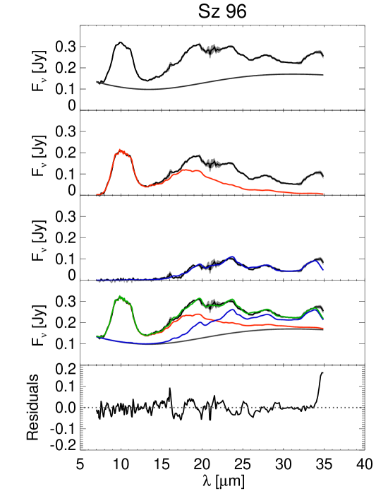
Figure 2: Detailed example of B2C modeling steps for the object Sz 96. From top to bottom: the original spectrum and the estimated continuum (top panel), the continuum substracted spectrum and the fit to the warm component (in orange, 2^nd panel), the residuals from the fit to the warm component and the fit to this cold component (in blue, 3^rd panel), the final fit to the entire spectrum (in green) and the various contributions (4^th panel), the relative residuals between the original spectrum and the final fit (last panel).

The successive steps of the B2C modeling approach are decomposed in Figure 2 for the illustrative case of Sz 96. The original spectrum ($F_{\nu,\rm obs}$) and the estimated continuum ($F_{\nu,\rm cont}$) are displayed in the top panel. Then, the fit to the 10 $\mu$m feature is performed ($F_{\nu,\rm warm}$, orange curve on second panel) and subtracted from the continuum-subtracted spectrum (black line on the third panel). It shows that, although the contribution of the first fit is not negligible up to $\sim$ 25 $\mu$m, a second, colder component is required to account for the large wavelength spectrum. The fit to the residuals ($F_{\nu,\rm cold}$, in blue on the third panel) is then computed, leading to an overall fit ($F_{\nu,\rm synt}$, green line) to the entire IRS spectrum as drawn in the fourth panel together whith all the contributions (continuum, warm and cold components). The last panel of Fig. 2 displays the final, relative residuals for the full fit of the IRS spectrum, calculated as follows: $(F_{\nu,\mathrm{obs}}-F_{\nu,\mathrm{synt}})/F_{\nu,\mathrm{synt}}$.

2.3 Fitting process

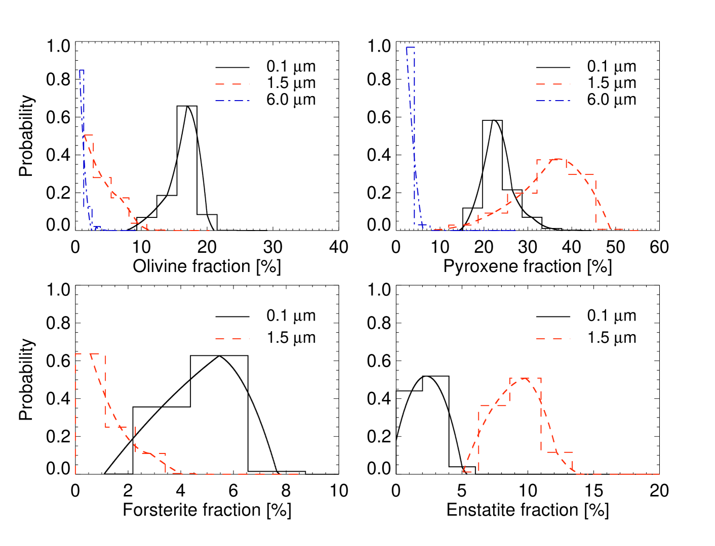
Figure 3: Examples of probabilities distributions for the fit to the Sz 96 spectrum. From the top left panel, clockwise, are displayed the probability distributions for the warm olivine, pyroxene, enstatite and forsterite grains. On each panel are represented 0.1 $\mu$m grains (black plain histogram), 1.5 $\mu$m grains (red dashed histogram) and 6.0 $\mu$m grains (blue dot-dashed histogram).

The parameter space has a high dimensionality in our problem and imposes a specific fitting approach to appreciate the reliability of the results. We develop in this paper a method based on a Bayesian analysis, combined with a Monte Carlo Markov chain (MCMC)–like approach to explore the parameter space.

Our procedure is built in order to randomly explore the space of free parameters ($2\times$ 13 dust compositions, 2 dust temperatures and 2 parameters for the continuum). We start with a randomly chosen initial set of parameters, then one of these parameters is randomly modified, while all the others remain unchanged. When the chosen parameter is related to the abundance of a grain species (the $M_{{\rm w},i}^{j}$ and $M_{{\rm c},i}^{j}$), the maximal value for the increment is 1% of the previous total mass for the considered component (warm or cold). When the chosen parameter is a temperature or the offset $O_{\nu,2}$, we allow increments of at most 4% of the previous temperature or the previous offset, respectively. These maximum values were chosen to obtain small enough increments and therefore explore continuously the parameter space.

For each set of parameters, a synthetic spectrum $F_{\nu,{\rm synt}}$ is calculated and the goodness of the fit to the observed spectrum is evalutated with a reduced $\chi^{2}_{\mathrm{r}}$. The parameter space exploration is therefore very much alike a MCMC approach, with two specificities: we only perform jumps for one parameter at a time, and second, the jumps are always accepted. After $n$ iterations (typically $n=800$), we set all the parameters to those that gave the lowest $\chi^{2}_{\mathrm{r}}$ among the $n$ previous iterations. This loop is done $m$ times (usually $m$ is also set to 800) and all the compositions, temperatures, offset and their associated $\chi^{2}_{\mathrm{r}}$ values are stored.

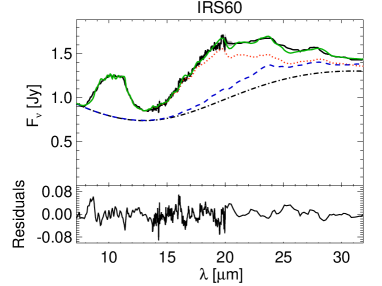
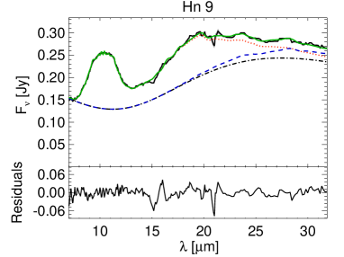
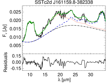
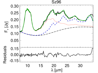
Figure 4: Examples of B2C fits over the entire IRS spectral range for four objects: IRS 60, Hn 9, SSTc2d J161159.8-382338 and Sz 96. The warm component is displayed in dotted orange line, the cold component in dashed blue line, and final fit to the entire spectrum in green. The dot-dashed grey line represents the continuum. The light grey enveloppe represents the 3-$\sigma$ uncertainty on the observed spectrum. For each star, the bottom panel shows the relative residuals.

The $n\times m$ reduced $\chi^{2}_{\mathrm{r}}$ values are transformed into probabilities assuming a Gaussian likelihood function ($\propto\exp(-\chi^{2}_{\mathrm{r}}/2)$) for Bayesian analysis. Marginalized probability distribution for each free parameter are then obtained by projection of these probabilities onto each dimension of the parameter space. The best fit to the observed spectrum among all the simulations (i.e., the one with the lowest $\chi^{2}_{\mathrm{r}}$ value), yields relative masses for all the dust species and grain sizes ($M_{{\rm w},i}^{j}$ and $M_{{\rm c},i}^{j}$ parameters in Eqs. 5 and 6) for both the warm and cold components, as well as best temperatures $T_{\mathrm{w}}$ and $T_{\mathrm{c}}$, which typically range between $200\,K$ and $300\,$K for the warm component, and between $70\,K$ and $150\,K$ for the cold one. The 1-$\sigma$ uncertainties on the parameters are derived from the probability distributions for each parameter. We over-sample each probability distribution to compute half-width at half maximum for both sides of the distribution, and derive minimum and maximum 1-$\sigma$ uncertainties. Figure 3 displays ten examples of well-peaked probability distributions, with their respective over-sampled distributions overplotted, for some parameters of the fit to the Sz 96 spectrum, indicating the parameters are constrained by the B2C fitting approach. Figure 4 displays four example spectra with their best fits (and residuals) over the entire IRS spectral range, showing that good fits can be obtained for spectra with different shapes. Spectral regions with high residuals mostly correspond to regions with low signal-to-noise ratio.

The robustness of the B2C procedure has been intensively tested and this work is reported in Appendix A. Using theoretical spectra we search for any possible deviations to the input dust mineralogy, that could either affect the inferred grain sizes or crystallinity fractions. The main result is that even if there is a slight deviation for a few individual cases, in a statistical point of view for a large sample, the B2C procedure is robust when determining the dust mineralogy.

3 Spectral decomposition of 58 T Tauri IRS spectra with the B2C model

We run the B2C compositional fitting procedure on 58 different stars (most of them being T Tauri stars, except BD+31 634 which is an Herbig Ae star), for which we obtained Spitzer/IRS spectra as part of the c2d Legacy program. The spectra are presented in Olofsson et al. (2009) and we refer to that paper for details about data reduction. The selection of the 58 objects out of 96 in Olofsson et al. (2009) is based on several criteria. First, some objects do not have Short-Low data therefore the amorphous 10 $\mu$m feature is not complete. Second, as the goal is to determine the dust mineralogy, we do not run the procedure for objects that do not show clear silicate emission features, or with peculiar spectra (e.g. cold disks like LkHa 330 or CoKu Tau /4, Brown et al. 2007). Finally, objects for which continuum estimation in the 5–7.5 $\mu$m spectral region was not possible using a power-law were eliminated.

The spectral range used for the fits is always limited to a maximum wavelength of 35 $\mu$m. The first reason of this choice is that the products of the c2d extraction pipeline are, for our sample, in average limited to 36.6 $\mu$m. In addition to this, the degrading quality of the end of the spectra, likely caused by the quality of the relative spectral response function used at these wavelengths, may lead to an over-prediction of the crystalline content, for the cold component. In a few cases, the spectra are rising for wavelengths larger than 35 $\mu$m, and the fitting procedure tries to match this rise with crystalline features (which are the only features strong enough in this spectral range). Finally, longer wavelengths may probe an even colder dust content and this would require the implementation of a third dust component in order to reproduce the entire spectral range. For all these reasons, we choose to limit the modeling to wavelengths smaller than 35 $\mu$m.

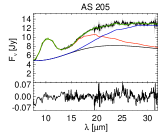
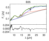
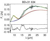
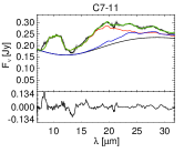
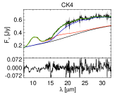
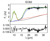
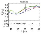
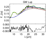
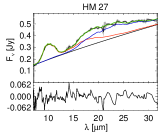
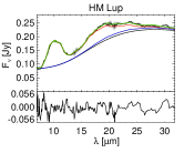
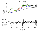
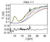
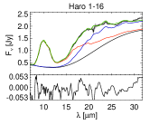
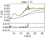
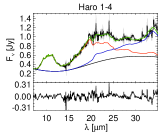
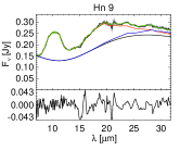
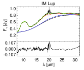
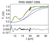
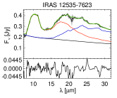
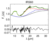
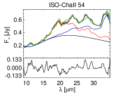
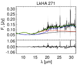
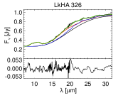
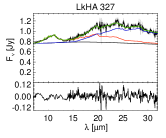
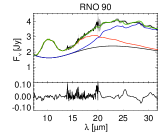
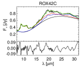
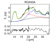
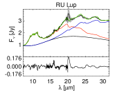
Figure 22: Fits to the 60 objects using the B2C procedure.

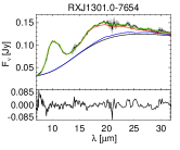
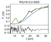
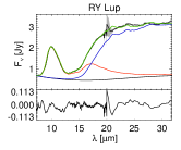
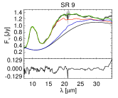
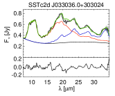
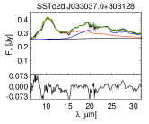
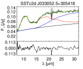
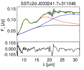
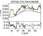
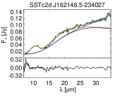
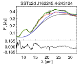
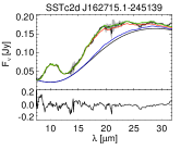
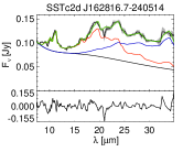
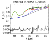
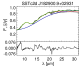
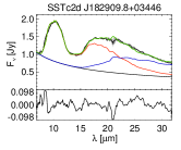
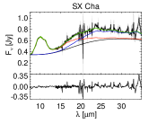
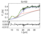
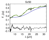
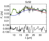
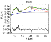
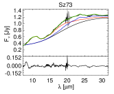
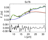
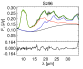
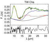
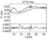
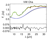
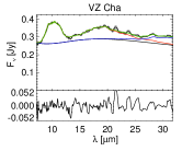
Figure 23: Continued

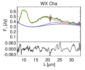
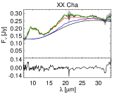
Figure 24: Continued

The source list and relative abundances for every object can be found in Table LABEL:tbl:silicate. Because of some degeneracy between amorphous olivine and pyroxene opacities, we sum their respective abundances to a single amorphous component. The final fits to the 58 IRS spectra are displayed in Figs 22–24.

3.1 Grain size properties

Figure 5: Mean grain sizes for the cold component as a function of the mean grain size for the warm component

3.1.1 Mean mass-averaged grain sizes

With the outputs of the “B2C” procedure for the 58 objects processed we have statistical trends on typical grain sizes necessary to reproduce the spectra. The mean mass-averaged grain sizes for the warm and cold components, $\langle a_{\rm warm}\rangle$ and $\langle a_{\rm cold}\rangle$, respectively, are calculated as follows:

$$\langle a_{\rm warm/cold}\rangle=\left(\sum_{j=1}^{\mathrm{N_{\rm sizes}}}a_{j}\sum_{i=1}^{\mathrm{N_{\rm species}}}M_{{\rm w/c},i}^{j}\right)\times\left(\sum_{j=1}^{\mathrm{N_{\rm sizes}}}\sum_{i=1}^{\mathrm{N_{\rm species}}}M_{{\rm w/c},i}^{j}\right)^{-1}$$ (8)

where $a_{1}=0.1\,\mu$m (small grains), $a_{2}=1.5\,\mu$m (intermediate-sized grains) and $a_{3}=6\,\mu$m (large grains), with the masses as defined in Eqs. 5 and 6. We further define $\langle a_{\rm warm/cold}^{\rm amo}\rangle$ and $\langle a_{\rm warm/cold}^{\rm cry}\rangle$ the mass-averaged grains sizes for amorphous and crystalline grains, respectively, in the warm or cold component.

We obtain a mean mass-averaged size of $\langle a_{\rm warm}\rangle=$ 2.28 $\mu$m for the warm component, and a comparable value of $\langle a_{\rm cold}\rangle=$ 2.02 $\mu$m for the cold component. Figure 5 shows that mass-averaged grain sizes for both components are uncorrelated with each other. In order to quantify the strength of the correlation, we compute the Kendall $\tau$ correlation coefficient and its associated probability $P$. The $\tau$ value denotes if there is any correlation or anti-correlation ($\tau=1$ or $-1$, respectively), and the $P$ probability corresponds to the significance probability (from 0 to 1, from the most to the less significant). Regarding the latter two quantities we obtain a Kendall $\tau$ value of -0.013 and a significance probability $P=$ 0.888. This overall suggests that the warm and cold disk regions considered in this study are independent, as both components show uncorrelated grain sizes in the inner and outer regions. This suggests that differential grain growth is not the sole process explaining the observed variations from object to object. This result is in line with the conclusions of Olofsson et al. (2009) and supporting the B2C model assumptions. In their study of 65 TTauri stars, Sargent et al. (2009) find that grains are larger in the inner regions compared to outer regions, and argue this difference can be explained by faster grain coagulation in the inner regions, where dynamical timescales are shorter. In our study, we find no strong evidence of such a difference (2.28 versus 2.02 $\mu$m). However Fig. 5 shows a larger dispersion in grain sizes for the warm component compared to the cold component. This could be a consequence of shorter dynamical timescales in the inner regions where grains are not frozen and will be strongly submitted to both coagulation and fragmentation processes, compared to the outer regions.

Additionally, we investigate the different mass-averaged grain sizes, for both the crystalline and amorphous grains. For the warm component, crystalline grains have a mean mass-averaged grain size of $\langle a_{\rm warm}^{\rm cry}\rangle=$ 1.14 $\mu$m while amorphous grains have $\langle a_{\rm warm}^{\rm amo}\rangle=$ 2.50 $\mu$m. For the cold component, we find $\langle a_{\rm cold}^{\rm cry}\rangle=$ 0.79 $\mu$m and $\langle a_{\rm cold}^{\rm amo}\rangle=$ 2.40 $\mu$m. As we did not include large crystalline grains in the fitting process, it is not surprising to obtain smaller mass-averaged sizes for the crystalline grains compared to amorphous grains. However this trend is supported by the results from Bouwman et al. (2008), for seven T Tauri stars.

Figure 6: Flaring indices $F_{30}/F_{13}$ as a function of the warm mass-averaged mean grain size.

3.1.2 Mass-averaged grain size versus disk flaring

As in Olofsson et al. (2009), we find a trend between $\langle a_{\rm warm}\rangle$ and disk flaring as measured by the flux ratio $F_{30}/F_{13}$ (fluxes in Jy integrated between $13\pm 0.5$ $\mu$m for $F_{13}$, and $30\pm 1$ $\mu$m for $F_{30}$). As illustrated in Figure 6, we find that large grains in the warm component are mostly present in flat disks, while smaller grains can be found in both flared or flat disks. This anti-correlation for the warm component has a Kendall correlation coefficient $\tau$ of -0.31 with a significance probability of 5.0$\times 10^{-4}$. This anti-correlation is still present, when considering only the warm amorphous grain sizes ($\tau=$ -0.32 with $P=$ 3.5 $\times 10^{-4}$). A similar anti-correlation has also been found by Bouwman et al. (2008), and by Watson et al. (2009a) in their Taurus-Auriga association sample.

Considering $\langle a_{\rm cold}^{\rm cry}\rangle$ as a function of the flaring degree ($F_{30}/F_{13}$), we search for a similar result as in Olofsson et al. (2009) where we found that small crystalline grains are preferentially seen in flattened disks, while large crystalline grains can be found in a variety of flat or flared disks. We did not find a similar trend from the outputs of the modeling, the correlation coefficient being $\tau=$ -0.040, with a significance probability of 0.66. According to this model, the size of the cold crystalline material seems to be strongly unrelated with the flaring degree of disks.

3.1.3 Flattened grain size distributions

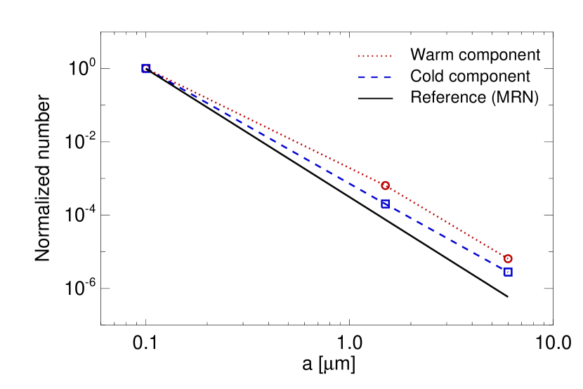
Figure 7: Grain sizes distribution, for warm (red circles and dotted line) and cold (blue squares and dashed line) component. The MRN reference distribution (-3.5 index) is the black plain line.

Since our spectral decomposition includes three grain sizes, for the amorphous species, we can evaluate the shape of the size distribution in the atmospheres of disks. Assuming a differential size distribution $\mathrm{d}n(a)=K_{a}a^{p}\mathrm{d}a$ where $K_{a}$ is a normalization constant, we approximate the number $N_{a}$ of grains of size $a$ with:

$$N_{a} \simeq \int_{a-\delta a/2}^{a+\delta a/2}\mathrm{d}n(a)=\frac{K_{a}}{1+p}\left[\left(a+\frac{\delta a}{2}\right)^{1+p}-\left(a-\frac{\delta a}{2}\right)^{1+p}\right]$$ (9)

$$\simeq K_{a}a^{p}\delta a$$ (10)

after a Taylor expansion to the first order of Eq. 9 about $a$ assuming $\delta a\ll a$. This shows that $N_{a_{i}}/N_{a_{k}}\simeq(a_{i}/a_{k})^{p}$ for two grain sizes $a_{i}$ and $a_{k}$, and therefore that relative numbers of grains can directly be used to evaluate the slope of the size distribution $p$. For each grain size, we compute the mean mass obtained from the B2C simulations, and then divide it by the corresponding volume ($\propto a^{3}$). We then normalize these relative grain numbers so that the total number of 0.1 $\mu$m-sized grain equals 1.

Fig. 7 shows the mean differential grain size distribution in normalized number of grains obtained following this procedure. On Fig. 7, the warm component is represented in filled circles, the cold component in open circles, and a reference MRN differential size distribution ($p=-3.5$) with a dashed line. Assuming power-law size distributions, we find $p$ indexes of $p_{\rm warm}=$-2.89 and $p_{\rm cold}=$-3.13 for the warm and cold components, respectively, indicating much flatter size distributions compared to the MRN size distribution. Two additional runs of the B2C procedure for the 58 objects allowed to confirm this trend, and to estimate uncertainties on the slopes. For the warm component, we typically find $p=-2.90\pm 0.1$, and $p=-3.15\pm 0.15$ for the cold component.

Because the $p$ indexes are larger or close to $-3$, an immediate consequence of this result is that the emission in disk upper layers is statistically dominated by the $\mu$m-sized grains in our stellar sample, especially for the warm component, and is largely independent of the minimum grain size of the size distribution as long as its value is small enough (submicronic, see discussion in Sec. 5.3 of Olofsson et al. 2009). This suggests that the flat, boxy $10\,\mu$m feature profile for most T Tauri stars discussed in terms of a depletion of small grains in Olofsson et al. (2009), is more precisely revealing a significant flattening of the size distribution, i.e. a relative lack of submicron-sized grains with respect to micron-sized grains, but not a complete depletion. This size distribution flattening is further discussed in Sec. 4.

3.2 Silicate crystals

3.2.1 The crystallinity paradox reexamined

Figure 8: Crystalline fraction of the cold component ($C_{\rm cold}$) as a function of the warm crystalline fraction ($C_{\rm warm}$).

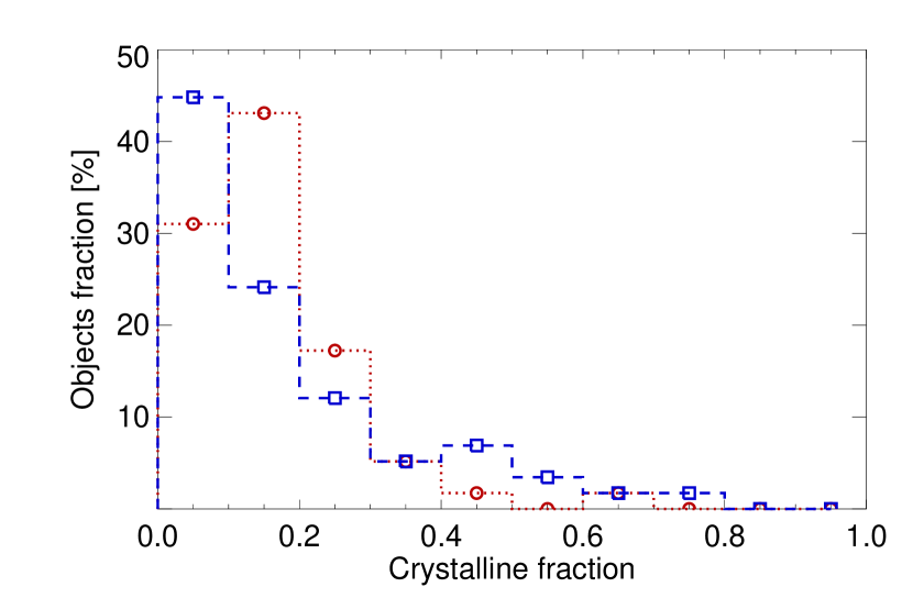
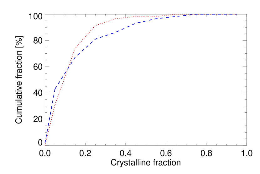
Figure 9: Left panel: crystalline distributions for warm component ($C_{\rm warm}$, red circles and dotted histogram) and cold component ($C_{\rm cold}$, blue squares and dashed hsitogram). Right panel: cumulative fractions of the crystallinity fractions, for the warm (red dotted line) and cold (blue dashed line) components.

Figure 8 shows the correlation between the warm and cold crystalline fractions (which we denote as $C_{\rm warm}$ and $C_{\rm cold}$, respectively, in the following), with Kendall’s $\tau=$0.25 and a significance probability $P=$ 5.8 $\times 10^{-3}$. While slightly dispersed, there is a tendency for a simultaneous increase of the crystallinity in both the warm and cold components. The crystalline distributions for the warm and cold components are displayed on the left panel of Fig. 9. For the warm component, the mean crystalline fraction is $\langle C_{\rm warm}\rangle\simeq$ 16%, while this fraction shifts up to $\langle C_{\rm cold}\rangle\simeq$ 19% for the cold component. Overall, these results show no significant difference between the crystalline fractions in both components.

These modeling results give us new insights concerning the crystallinity paradox identified observationally in Olofsson et al. (2009). The crystallinity paradox expresses the fact that crystalline features at long wavelengths are $\sim$ 3.5 times more frequently detected than those at shorter wavelengths. Using simple models of dust opacities, we concluded that a contrast effect (i.e. the strong 10 $\mu$m amorphous feature masking smaller crystalline features) could not be accounted for the low detection frequency of crystalline features in the 10 $\mu$m range, a result valid for crystallinity fraction larger than 15% for 1.5 $\mu$m grains (Olofsson et al. 2009). For lower crystallinity values, we indeed showed that the synthetic spectra computed in Olofsson et al. (2009) were not representative of the observations. This contrast effect could therefore not be constrained for low-crystallinity fractions, where most of our objects lie for the warm component, according to Fig. 9. With the outputs of the modeling procedure, we can investigate this issue with a new look. Right panel of Fig. 9 shows the cumulative fractions as a function of the crystallinity fractions. Even if there are a few differences between the warm (red dotted) and cold (blue dashed) components, the two cumulative fractions display a very similar behavior that cannot solely explain the crystallinity paradox that we derived from the observations. This therefore means that, with this modeling procedure, a contrast issue around 10 $\mu$m is required to match the observations described in Olofsson et al. (2009). In other words, for some objects, few crystalline grains are required to reproduce the 10 $\mu$m feature, but these grains do not produce strong features (on top of the amorphous feature) that can easily be detected in the spectra. Still, the left panel of Fig. 9 shows that the cold crystalline distribution is wider than the warm distribution. For the warm component, 3.5% of the objects have a crystallinity fractions larger than 40%, while this fraction shifts up to 13.8% for the cold component. This overall means that in a few cases, we see more crystalline grains in the cold component compared to the warm component, as result also found by Sargent et al. (2009)

3.2.2 Crystallinity versus disk and stellar properties

We also search for correlations between disk flaring proxies and crystallinity. We find no striking correlations regarding the disk flaring indexes $F_{30}/F_{13}$ and warm crystalline fraction $C_{\rm warm}$ ($\tau=$ -0.11 with a significance probability $P=$ 0.23). Flared or flat disks present a wide range of crystalline fractions, with a strong dispersion. We find similar results, with an important dispersion, for the flaring index versus cold crystalline fraction $C_{\rm cold}$ ($\tau=$ -0.16 with a significance probability $P=$ 0.08), meaning that crystallinity fraction of the cold component does not strongly depend on the disk flaring.

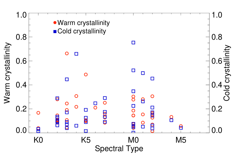
Figure 10: Crystalline fraction for the warm ($C_{\rm warm}$, open red circles) and the cold ($C_{\rm cold}$, open blue squares) components, as a function of the spectral types.

Figure 10 displays the dependence of crystalline fractions for both the warm ($C_{\rm warm}$, red open circles) and cold components ($C_{\rm cold}$, blue open squares) as a function of the spectral type, for stars between K0 and M5. We find no correlation for the warm component with the spectral type ($\tau=$ 0.13 with $P=$ 0.20), suggesting that the degree of crystallization does not depend upon the spectral type (in the explored range), and that crystallization processes are very general for TTs. This result is in good agreement with Watson et al. (2009a), who find no correlation between crystallinity and stellar luminosity or stellar mass. On the other hand, Watson et al. (2009a) only studied the cold disk regions crystallinity via the presence of the 33.6 $\mu$m forsterite feature. Using the outputs of our B2C procedure, we are able to better quantify the crystalline fraction of the cold component, and we do not find any correlation of $C_{\rm cold}$ with spectral type, the dispersion being too large ($\tau=$ 0.12 with $P=$ 0.24), thereby confirming the result by Watson et al. (2009a).

3.2.3 Dust evolution: coagulation versus crystallization

Figure 11: Warm crystalline fraction $C_{\rm warm}$ versus warm mass-averaged grain size $\langle a_{\rm warm}\rangle$.

Dust is evolving inside circumstellar disks, either in size or in lattice structure, in particular through coagulation and crystallization. To investigate possible links between these two phenomena, we search for correlations between grain sizes, for amorphous and crystalline dust contents ($\langle a_{\rm warm/cold}\rangle$), as a function of crystalline fractions, in both the warm and cold components ($C_{\rm warm/cold}$).

We find no evidence that grains are growing and crystallizing at the same time in the warm component. Considering $\langle a_{\rm warm}\rangle$ and $C_{\rm warm}$ values, we obtain the following coefficients: $\tau=$ -0.038, with a significance probability equal to 0.67. This result is displayed in Fig. 11. We obtain an even less favorable correlation coefficients for the cold component ($\tau$ = 0.013 with $P=$ 0.89). This overall indicates that the processes that govern the mean size of the grains and their crystallinity are independent phenomena in disks.

We also search for correlations between the amorphous and crystalline dust contents for the two components, to see how they evolve with respect to each others. Based on our B2C spectral decomposition, we find no significant correlations between the several amorphous or crystalline dust populations.

3.2.4 Enstatite, forsterite and silica

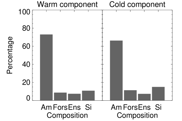
Figure 12: Mean composition for warm and cold components according to the results of the 58 objects processed.

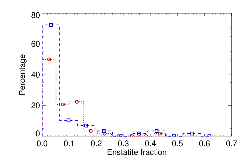
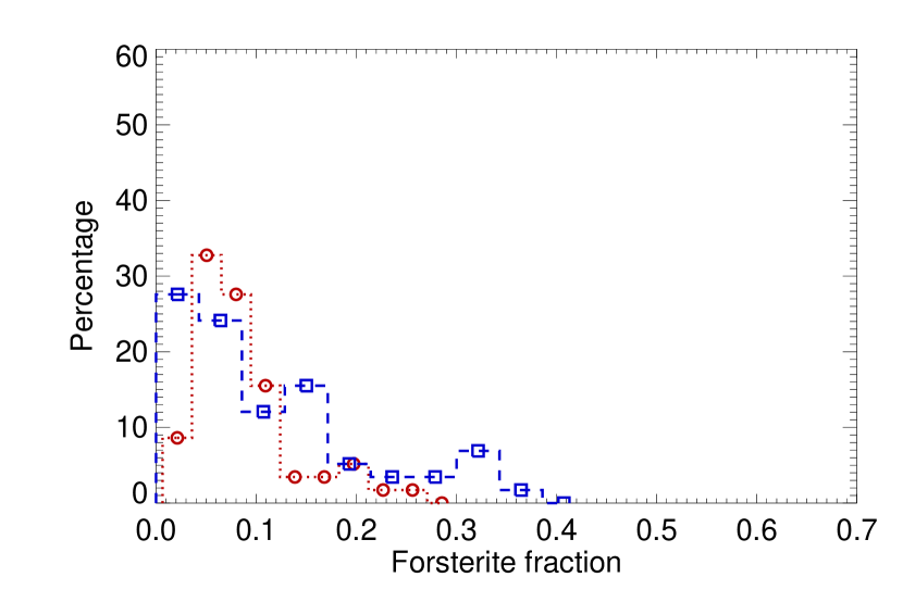
Figure 13: Distribution for the warm (red circles and dotted histogram), cold (blue squares and dashed histogram) for enstatite (left panel) and forsterite (right panel) crystalline abundances.

Bouwman et al. (2008) find that enstatite dominates in the innermost warm regions over forsterite, and on the other side that forsterite is the dominant silicate crystal in the cooler outer regions. Fig. 12 shows the mean composition we obtain for the 58 objects, for both components (warm and cold). As amorphous pyroxene and amorphous olivine spectral signatures are very similar, we merge together their relative contributions. Regarding the crystalline content, even if there is no clear predominance of forsterite or enstatite masses for the warm component (8.7% vs. 7.4% respectively), for the cold component forsterite appears more abundant than enstatite (11.4% vs. 7.4% in mass). In order to have more details on the presence or absence of these two crystals, Figure 13 shows the distribution for the enstatite and forsterite abundances (left and right panel, respectively), for the warm and cold components (filled circles and open circles, respectively). No predominance of either enstatite or forsterite is found in the warm component, while forsterite seems to be more frequent than enstatite in the cold component. Similar distributions are found by Sargent et al. (2009) regarding the warm and cold forsterite and enstatite.

We search for correlations between the masses of the warm or cold enstatite populations, and warm or cold forsterite populations. We find a correlation between warm enstatite and warm forsterite grains, with a Kendall’s $\tau$ value of 0.33 and with a significance probability $P$ equal to 2.7$\times 10^{-4}$. This trend tends to confirm the results displayed in Fig. 12: the crystallisation processes in the warm component do not favor the formation of one or the other crystals. We also find a correlation between the relative masses of warm enstatite grains and cold forsterite grains, with $\tau=$ 0.31 and $P$ equal to 7.0$\times 10^{-4}$. This tends to indicate that the enrichment in crystalline grains in the disk is global within $\sim$10 AU, and not local.

Knowing that forsterite and silica can interact with each other to form enstatite ($\mathrm{Mg_{2}SiO_{4}}+\mathrm{SiO_{2}}\to 2\mathrm{MgSiO_{3}}$), we search for correlations between the relatives masses of forsterite, enstatite and silica in both components. We may expect to find an anti-correlation between the presence of enstatite and silica, as silica disappears from the disk medium in the above reaction. We did not find any striking trend between all the masses, even when considering only small and intermediate-sized grains (0.1 and 1.5 $\mu$m). This suggests that the reaction between forsterite and silica is not the main path for enstatite production.

3.3 Sample homogeneity

Table 1: Cloud-to-cloud variations for several parameters from the spectral decomposition.

Cloud	Number	$\alpha_{\rm warm}$	$\alpha_{\rm cold}$	$\langle C_{\rm warm}\rangle$	$\langle C_{\rm cold}\rangle$
Chamaleon	16	-2.97	-3.05	18.4	19.9
Ophiuchus	14	-3.02	-3.10	16.0	19.0
Lupus	13	-2.96	-3.06	16.6	20.8
Perseus	8	-2.60	-3.27	13.2	12.3
Serpens	5	-2.80	-3.11	11.6	14.3
Taurus	1	-2.84	-3.00	30.3	52.1

The studied stellar sample is drawn from several star forming regions. It may therefore be interesting to see if any cloud-to-cloud variations can be observed. The 58 Class II objects are distributed among 6 different clouds: Chamaleon, Ophiuchus, Lupus, Perseus, Serpens and Taurus (except for IRAS~08267-3336 which is an isolated star). Table 1 shows several results as a function of the corresponding clouds: the number of objects, the grain-size distribution slopes for the warm and cold components, and both the warm and cold crystallinity fractions. The results for the Perseus, Serpens and Taurus clouds are not statistically significant, given the low-statistics number of stars for these regions. On the other side, the three other clouds show very similar behavior for all the considered results. The grain size distributions and crystallinity fractions are very close to each other (with a number of objects between 13 and 16 per cloud).

Recently, Oliveira et al. (2010) studied the amorphous silicate features in a large sample of 147 sources in the Serpens, and compared their results with the Taurus young stars. That study, along with the results from Olofsson et al. (2009), show that the 10 $\mu$m feature appears to have a similar distribution of shape and strength, regardless of the star forming region or stellar ages. In terms of silicate features, the stellar sample analyzed in this study is therefore representative of a typical population of TTauri stars.

4 Discussion

4.1 Implications for the dust dynamics in the atmospheres of young disks

In Olofsson et al. (2009), we discussed the impact of a size distribution on the shape of the $10\,\mu$m feature, and could not disentangle between two possibilities to explain the flat, boxy $10\,\mu$m feature profile that is characteristic of micron-sized grains. One possibility was that the grain size distribution is close to a MRN-like distribution ($p=-3.5$), extending down to sizes of at least several micrometers, with the consequence that the Spitzer/IRS observations would then probe a truncation of the size distribution at the minimum grain size (of the order of a micrometer). A second possibility implied a differential size distribution $\mathrm{d}n(a)\propto a^{p}\mathrm{d}a$ that departs from a MRN-like distribution, being much flatter and with an index $p$ close to, or larger than $-3$ to get the dust absorption/emission cross sections dominated by grains with size parameters $2\pi a/\lambda$ close to unity.

By model fitting 58 IRS spectra of T Tauri stars, we find a general flattening of the grain size distribution ($p_{\rm warm}\simeq$ -2.9 $p_{\rm cold}\simeq$ -3.15) in the atmospheres of disks around T Tauri stars with respect to the grain size distribution in the ISM up to about 10 AU (this effect being stronger for the inner regions of disks). Our results suggest that the frequently observed boxy shape of the $10\,\mu$m feature is rather due to the slope of the size distribution, than to a minimum grain size in the disk atmospheres close to a micrometer. This finding very much relaxes the need for a sharp, and quite generic truncation of the size distribution at around one micrometer as proposed in Olofsson et al. (2009). Nevertheless, radiation pressure and/or stellar winds which had been proposed to explain such a cut-off are likely to operate anyway, and may thus contribute to the flattening of the size distribution by removing a fraction of the submicron-sized grains. This would furthermore help transporting crystalline grains outwards.

An alternative explanation for the size distribution flattening involves an overabundance of micrometer-sized grains with respect to the submicron-sized grains. At first glance, this situation may sound counterintuitive as micrometer-sized grains are more prone to settle toward the disk midplane which would, in turn, tend to steepen the size distribution in disk atmospheres. This ignores that both turbulent diffusion and collisions between pebbles may complicate this picture, and may even possibly revert this trend by supplying the disk atmospheres with micrometer-sized (and larger) grains. Therefore, the IRS observations may in fact indicate that coagulation and vertical mixing are slightly more efficient processes to supply grains in disk atmospheres than fragmentation, resulting in an overabundance of micrometer-sized grains compared to an ISM-like distribution. This situation may last over most of the TTauri phase.

Interestingly, Lommen et al. (2010) also found a flattening of the grain size distributions for T Tauri stars, probed by the millimeter slope of the SED. They found a tentative correlation between the shape of the 10 $\mu$m feature and the mm slope for a large sample of sources, with flatter 10 $\mu$m feature being associated with shallower mm slopes. Similarly, Ricci et al. (2010) also find grain size distributions flatter than in the ISM, with 3 mm PdBI observations of T Tauri stars in the Taurus-Auriga star forming region. Therefore, the size distribution flattening in disk atmospheres may extend to deeper and more distant regions, and to larger grains sizes than those probed by mid-IR spectroscopy.

4.2 Silicate crystallization and amorphization

In this study, we have been able to quantify the fraction of crystals for both the warm and cold components. In Olofsson et al. (2009), we identify a crystallinity paradox expressing the fact that crystalline features are much more frequently detected at long wavelengths compared to short wavelengths. By building crystallinity distributions with the results from the spectral decomposition, we find that even if the cold crystalline distribution is slightly broader than the warm distribution, they both show a similar behavior (see right panel of Fig.9). Therefore, this may suggest that the observational crystallinity paradox could be the consequence of a combined effect: relatively low crystalline fractions ($\leq$15-20%) for a great number of the TTauri stars, and a contrast issue at short wavelengths preventing the direct identification of weak crystalline features on top of the 10 $\mu$m amorphous feature. Nevertheless, it is noteworthy that correcting for the contrast issue through B2C spectral decomposition does not revert the trend, but instead makes the distribution of crystals in the warm and cold disk regions quite similar.

In order to explain the non negligible crystallinity fractions obtained for the cold component (up to 70% in a few cases, e.g. Fig. 8), there is a strong need for radial outward transport, assuming that the only source of production of crystals is thermal annealing or gas-phase condensation/annealing, taking place in the inner regions of disks. Several models have shown that such mechanism is likely to happen in circumstellar disks around active stars (see Keller & Gail 2004 or Ciesla 2009). According to Ciesla (2009), for an accretion rate larger than 10^-7 M${}_{\odot}/yr$, grains can be transported to distances out to 20 AU in about $\sim$ 10⁵ years. A result in line with the 2D time-dependent disk model described in Visser & Dullemond (2010). However given the relatively young ages of our stellar sample ($\sim$ few Myrs), and the rather high accretion rate required (10^-7 M${}_{\odot}/yr$), we cannot assess that radial transport is the only mechanism responsible for the strong similarity of both warm and cold crystallinity distributions. This instead suggests that other crystallization processes are necessary, that must take place in the outer regions of disks. A theoretical model, detailed in Tanaka et al. (2010), shows that depending on the gas density, crystallization can take place with typical temperature of a few hundred Kelvin. Such process can be triggered in the outer regions by nebular shocks (Desch & Connolly 2002) which lead to graphitization of the carbon mantle providing the latent heat for silicate crystallization.

However, crystallization by thermal annealing is likely to happen on very short timescales (few hours at $T\sim 1000$ K, according to laboratory measurements, see Hallenbeck et al. 1998). Therefore, one can expect to observe higher crystallinity fractions in the inner warm regions compared to the outer cold regions. One possible explanation to this issue may rely on the importance of accretion activity and on amorphization processes of crystals that are preferentially taking place in the inner regions of disks, as tentatively proposed by Kessler-Silacci et al. (2006) and Olofsson et al. (2009), and recently discussed in more detail in Glauser et al. (2009). This possibility is further supported by the results of Ábrahám et al. (2009) who studied the TTauri star EX Lup with IRS, at two different epochs separated by a three-year time span, first in a quiescent phase (see spectrum in Kessler-Silacci et al. 2006), and then two months after an optical outburst driven by an increase of the mass accretion rate. They find an increase of crystallinity caused by this outburst in the inner disk regions, supposedly due to thermal annealing of amorphous silicates. The authors did not find any colder crystals in the outer component after the outburst, and therefore excluded shock heating at larger distances. This study shows that, obviously, the accretion activity may have a strong impact on the dust chemistry in circumstellar disks. Recently, Glauser et al. (2009) identified an anti-correlation between X-ray luminosity of the stars and crystalline fraction for the warm disk component ($C_{\rm warm}$ in Sec.3.2). The authors performed a decomposition fit to the $10\,\mu$m feature for a stellar sample of 42 TTauri stars, and find an anti-correlation between $C_{\rm warm}$ and X-ray luminosities for a subsample of 20 objects with ages between 1 and 4.5 Myr. This anti-correlation suggests that the stellar activity and energetic ions from stellar winds, traced by X-ray flux, can amorphize crystalline grains in disk atmospheres due to high-energy particles.

In a similar approach as Glauser et al. (2009), we attempt to investigate the impact of high-energy particles, assumed to be traced by X-ray luminosity, on the disk mineralogy. Table 2 displays the X-ray luminosities (in units of erg.s^-1) available in the literature or obtained by fitting the spectra from the Second XMM-Newton serendipitous source catalogue (Watson et al. 2009b) with the X-ray emission from one or two-temperature plasma combined with photoelectric absorption, for a subset of 17 objects among our stellar sample analyzed with the B2C compositional fitting model. The low overlap between X-ray observations with the c2d sample can be explained by the different observation strategies: X-ray campaigns are mostly targetting dense cores while our observations are located at the periphery of the clouds. Fig. 14 displays the crystalline fraction $C_{\rm warm}$ for the warm component inferred with the B2C procedure, as a function of the X-ray luminosity. The associated Kendall $\tau$ value is 0.16 with a significance probability $P=$ 0.36, suggesting a dispersed weak trend, if any. To confirm any weak trend, we would need to have more measurements below about 2 $\times$ 10²⁹ erg.s^-1. Above this luminosity value no trend is visible. Still, we observe that objects with high X-ray luminosities seem to have higher crystalline fractions, which seems at first in contradiction with the conclusion by Glauser et al. (2009). Given the limited number of objects for which we have X-ray data in our sample, however, we were not able to perform any age selection as in Glauser et al. (2009).

Table 2: X-ray luminosities for a subset of our stellar sample.

Star Name	Satellite	LX [erg/s]	Ref
HM 27	ROSAT	$<$ 6.3$\times 10^{28}$	Feigelson et al. (1993)
LkHA 271	CXO	1.3$\times 10^{28}$	Getman et al. (2002)
Hn 9	XMM	1.6$\times 10^{29}$	Robrade & Schmitt (2007)
TW Cha	ROSAT	4.0$\times 10^{29}$	Feigelson et al. (1993)
IM Lup	XMM	4.2$\times 10^{29}$	this study
CK4	CXO	4.4$\times 10^{29}$	Giardino et al. (2007)
SSTc2d J162715.1-245139	XMM	4.6$\times 10^{29}$	Ozawa et al. (2005)
SX Cha	XMM	4.7$\times 10^{29}$	this study
XX Cha	XMM	1.0$\times 10^{30}$	Robrade & Schmitt (2007)
VZ Cha	XMM	1.3$\times 10^{30}$	Robrade & Schmitt (2007)
V710 Tau	XMM	1.4$\times 10^{30}$	Güdel et al. (2007)
WX Cha	XMM	1.5$\times 10^{30}$	Stelzer et al. (2004)
SR 9	ROSAT	2.5$\times 10^{30}$	Casanova et al. (1995)
RU Lup	XMM	3.1$\times 10^{30}$	this study
C7-11	XMM	5.9$\times 10^{30}$	Stelzer et al. (2004)
Sz96	XMM	6.2$\times 10^{30}$	this study
VW Cha	XMM	9.3$\times 10^{30}$	Stelzer et al. (2004)

Figure 14: Crystalline fraction for the warm component ($C_{\rm warm}$) as a function of the X-ray luminosities.

4.3 Strength of the 10 $\mu$m feature, a proxy for grain size ?

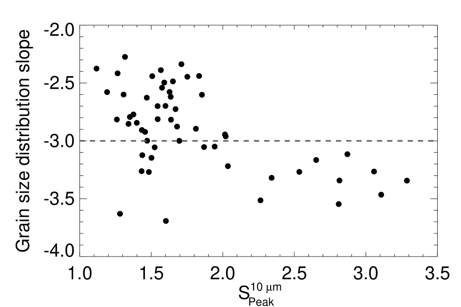
Figure 15: Left panel: Mass-averaged grain sizes for the warm component, as a function of the strength of the 10 $\mu$m feature ($S_{\mathrm{Peak}}^{10\mu m}$). Right panel: power-law index $p$ of the grain size distribution as a function of $S_{\mathrm{Peak}}^{10\mu m}$.

The strength $S_{\mathrm{Peak}}^{10\mu m}$ of the 10 $\mu$m feature has been commonly used in previous studies (e.g. van Boekel et al. 2005, Kessler-Silacci et al. 2006, Olofsson et al. 2009) as a proxy for grain size, small $S_{\mathrm{Peak}}^{10\mu m}$ values tracing large (micrometer-sized) grains, while larger $S_{\mathrm{Peak}}^{10\mu m}$ would be tracing smaller (submicron-sized) grains. In a recent paper, Watson et al. (2009a) instead attribute the diversity of strengths of the 10 $\mu$m feature to a combination of sedimentation and an increase of the crystallinity degree (as in Sargent et al. 2009). With the outputs of our B2C spectral decompositional procedure, we revisit the interpretation of the strength of the 10 $\mu$m feature as a proxy for grain size.

The left panel of Fig. 15 displays the correlation between the mass-averaged grain size for the warm grains ($\langle a_{\rm warm}\rangle$) and the strength of the 10 $\mu$m feature ($S_{\mathrm{Peak}}^{10\mu m}$). We find a Kendall $\tau$ correlation coefficient of about -0.30 with a significance $P$ probability smaller than 1.1 $\times 10^{-3}$, showing that grain size is well traced by the strength of the feature. It is noteworthy to point out that Sargent et al. (2009) find a different result regarding these two quantities, in their spectral decomposition analysis of 65 T Tauri stars. As shown in the review by Watson (2009), based on Sargent et al. (2009) results, they find a correlation coefficient of 0.08 with a significant probability of 0.55. This means, according to their model, that the strength of the 10 $\mu$m feature is not correlated with the presence of large grains. More precisely, they find that seven objects among their sample with the smallest 10 $\mu$m feature strength, can be reproduced with low abundances of large grains. However, our opposite result is supported by several points: we successfully checked for all dependencies that could lead to a possible overestimate of the grain sizes (e.g the continuum offset $O_{\nu_{2}}$) and we show in App. A.1, based on the analysis of synthetic spectra, that we may eventually underestimate the grain sizes in the warm component rather than over-estimate it (underestimated by $7\pm 11$% with respect to the input value). This deviation ($\langle a\rangle/\langle a_{\mathrm{inp}}\rangle$) is furthermore independent of the strength of the 10 $\mu$m feature ($S_{\mathrm{Peak}}^{10\mu\mathrm{m}}$), with a $\tau$ value of -0.06 and a significance probability of 0.52.

We also search for a correlation between the warm crystalline fraction $C_{\rm warm}$ and the strength of the 10 $\mu$m feature ($S_{\mathrm{Peak}}^{10\mu m}$), and find a highly dispersed relation between the two quantities. Fig. 16 shows that the distribution is flat ($\tau=$ -0.15 with a significance probability of 0.10), which suggests that crystallization cannot be the sole explanation for the diversity of 10$\,\mu$m feature strengths. This is in line with the results by Bouwman et al. (2008) who do not find any correlation between these two quantities in their seven T Tauri star sample.

As mentioned in Olofsson et al. (2009) and in this paper, the grain size distribution in the upper layers of disks has a strong impact on the 10 $\mu$m feature strength. The right panel of Fig. 15 shows the power-law indexes $p$ of the size distributions (calculated as in Sec. 3.1.3), as a function of the $S_{\mathrm{Peak}}^{10\mu m}$ values. We find an anti-correlation ($\tau=$ -0.28 with $P=$ 2.3 $\times 10^{-3}$), indicating the shape of the 10$\,\mu$m feature is indeed related to the slope of the grain size distribution. In fact we see two different regimes appearing: the small $S_{\mathrm{Peak}}^{10\mu m}$ values mostly correspond to objects with slopes $p$ larger than $-3$ (dashed horizontal line on the figure), while objects with large $S_{\mathrm{Peak}}^{10\mu m}$ values essentially have slopes $p$ smaller than $-3$. This points in the same direction as previously discussed, namely that the variation in $S_{\mathrm{Peak}}^{10\mu m}$ may to a large extent trace the variation in the slope of the size distribution. Not surprisingly, we find a very strong correlation between the mean mass-averaged grain size and the slope of the grain size distribution, with $\tau=$ 0.79 and a significance probability below $10^{-38}$.

Figure 16: Crystalline fraction for the warm component ($C_{\rm warm}$), as a function of the strength of the 10 $\mu$m feature ($S_{\mathrm{Peak}}^{10\mu m}$).

5 Summary and conclusion

In this paper, we present a large statistical study of the dust mineralogy in 58 proto-planetary (Class II) disks around young solar analogs. We develop a robust routine that reproduces IRS spectra over their entire spectral range (5–35 $\mu$m), with a MCMC-like approach coupled with a Bayesian inference method. This procedure explores randomly the parameter space and reproduces IRS spectra using two independent dust populations: a warm and a cold component, arising from inner and outer regions from disks, respectively. This 2-component approach is supported by our previous statistical analysis of the silicate features in Olofsson et al. (2009). This B2C procedure has been tested over synthetic spectra giving, statistically speaking, coherent and reproducible results. In its current form, the B2C model allows to derive relative abundances for 5 different dust species, 3 different grain sizes for the amorphous grains, 2 sizes for the crystalline grains, for both inner regions ($\leq 1$ AU) and outer regions ($\sim 10$ AU) of disks. Based on the modeling of the 58 IRS spectra of TTauris stars, we find the following results:

1. The grain sizes in the inner and outer regions of disks are found to be uncorrelated, reinforcing the idea of two independent components probed by IRS. However, crystallinity fractions in warm and cold components are correlated to each other, indicative of a simultaneous enrichment of crystals within the first 10 AU of disks. This suggests that dynamical processes affecting the size distribution are essentially local rather than global, while crystallization may rather trace larger scale phenomena (e.g. radial diffusion). Finally, we find that grain size and crystallinity fraction are two independent quantities with respect to each other in both the warm and cold components.

2. We quantify the growth of grains compared to the ISM. We find a significant size distribution flattening in the upper atmospheres of disks probed by IRS, compared to the MRN grain size distribution. While the MRN size distribution has a power law index $p=-3.5$, we find flatter distributions for both the inner regions ($\langle p\rangle=-2.90\pm 0.1$), and the outer regions ($\langle p\rangle=-3.15\pm 0.15$). This explains why the IR emission of T Tauri stars studied using Spitzer-IRS is dominated by $\mu$m-sized grains, despite the possible presence of significant amounts of submicron-sized grains. The $S_{\rm peak}^{10\mu m}$ value turns out to be a proxy of the slope of the grain size distribution. This finding, combined with recent similar results from observations at millimeter wavelengths, suggests that the size distribution flattening is not confined to the disk upper layers but may extend to deeper and more distance disk regions, and larger grains.

3. We reexamined the crystallinity paradox identified in Olofsson et al. (2009), by building crystallinity distributions for the warm and cold components. The mean crystallinity fractions are 16 and 19% for the warm and cold components, respectively. Even if the crystalline distribution for the cold component is slightly wider compared to the warm component, both distributions show a very similar behavior, suggesting the silicate crystals are well mixed within the first 10 AU of disks around T Tauri stars. According to the B2C model, the 3.5 times more frequently detected crystalline features at long (20-30 $\mu$m) than at short ($\sim$10 $\mu$m) wavelengths arises from the combination of rather low crystalline fractions ($\leq$15-20%) for many T Tauri stars, and a contrast effect that makes the crystalline features more difficult to identify at around 10 $\mu$m where the strong amorphous feature can hide smaller crystalline features.

4. We see a trend where flared disks (high $F_{30}/F_{13}$ values) tend to preferentially show small warm grains while flat disks (small $F_{30}/F_{13}$) show a large diversity of grain sizes. We do not find any correlations between the disk flaring and the crystallinity, meaning that the presence of such crystals is not related to the shape of the disks.

5. We find no predominance of any crystal species in the warm component, while forsterite seems to be more frequent compared to enstatite in the cold component. Regarding the different dust compositions, we find no evidence of correlations between them, except for the warm enstatite and forsterite grains, suggesting that the crystallisation processes in the inner regions of disks do not favor any of the two crystals. We find no link between silica and enstatite as one may expect if the main path for enstatite production would be the reaction between silica plus forsterite.

6. We do not find any striking correlation between spectral type and warm or cold crystallinity fraction. We do not either find any correlation between X-ray activity and crystallinity. As suggested by Watson et al. (2009a), the time variability in young objects may be responsible for erasing most of the correlations regarding dust mineralogy.

Appendix A Validation

A.1 Procedure validation

We evaluate the robustness of our procedure by fitting synthetic spectra with known abundances, temperatures and continua. This allows to check whether these quantities could be recovered when the spectra are processed with the B2C procedure. To this end, we used the best fit, synthetic spectra for the 58 objects analyzed in this paper (and presented in Sec. 3), as fake, but representative observations for serving as inputs to our B2C procedure. We reconstructed these synthetic spectra using the outputs of the fitting process on the original data. Namely, the same continuum emission, the same relative abundances for the dust species and their corresponding temperatures. The uncertainties chosen for the synthetic spectra are those of the original observed spectra.

Fig. 17 shows the ratio between the output and input crystallinity, as a function of the ratio between the output and input grain sizes, for both the warm and cold components. The plot shows ratios of about 1 on both axis, especially for the cold component (blue squares on the figure), suggesting some best fits obtained with the procedure may not be unique. But from a statistical point view, the B2C procedure produces reproducible results as the mean ratios between output and input quantities remain close to 1 (vertical and horizontal bars on the figure).

More precisely, the warm component crystallinity is slightly overestimated by 22% with a dispersion (i.e. the standard deviation) about this value of 30 %. The inferred cold component crystallinity is satisfactorily reproduced at the 2% level with respect to the input value, and the dispersion, 35%, is rather similar to that for the crystallinity of the warm grains. The mean mass-averaged size of the warm grains is slightly underestimated by 7$\pm$11% with respect to the input value, while the mean mass-averaged size of the cold grains is well reproduced but with a larger dispersion ( 1$\pm$32%).

A closer look at the dispersion of the calculated crystalline fraction as a function of the input crystallinity is shown in Figure 18 for the 58 fits to synthetic spectra, for both the warm (red open circles) and cold (blue open squares) components. The over-estimation of the warm component crystalline fractions seen in Fig. 17 is mostly visible for objects with low-crystalline fractions (below 20%). For the cold component, it actually tends to be rather underestimated for large crystalline fractions (above $\sim$40%). The overall trend for both the warm and cold components is that the dispersion raises with the decreasing crystallinity. This finds an explanation in the fact that objects showing high crystalline fractions display strong, high-contrast crystalline features that are less ambiguously matched by theoretical opacities than objects with lower crystalline fractions.

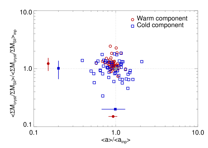
Figure 17: Results for the fits to the 58 synthetic spectra to test our “B2C” procedure. The $x$-axis shows the dispersion in grain size (ratio of inferred over input mean mass-averaged grain sizes) and the $y$-axis the ratio between inferred and input crystallinity. Red open circles correspond to the warm component, and blue open squares to the cold component. The filled circles are mean values, with error bars corresponding to standard deviations.

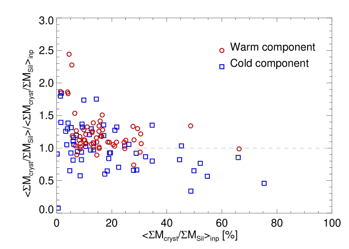
Figure 18: Ratios between output over input crystallinity fractions as a function of the input crystallinity fractions, for the fits to the 58 synthetic spectra. Red open circles are results for the warm component and blue open squares are for the cold component.

A.2 Influence of the continuum on the cold component

The continuum estimation is a critical step when modeling spectra, especially for the cold component, and may contribute to the larger uncertainties on the inferred cold component crystallinities and sizes discussed in previous subsection. The continuum may affect the model outputs in the following way: a high-flux continuum in the 20–30$\,\mu$m spectral range leaves very little flux to be fitted under the spectrum, possibly leading to a composition with few large and/or featureless grains. A low-flux continuum could, on the other hand, lean toward large/featureless grains to fill the flux left. We therefore examine if (whether) such trends are present in the results of our B2C procedure (or not) for the cold component.

We quantify the level of continuum by integrating the continuum-substracted spectra between 22 $\mu$m and 35 $\mu$m ($x$-axis on Fig. 19). Low-flux continua have high integrated fluxes and are located on the right side of the plot in Fig. 19, the high-flux continua being on the left side. The left panel of Fig. 19 shows the crystalline fraction for the cold component, as a function of the integrated flux left once the continuum is substracted. The trend low continuum – low crystalline fraction is visible for the highest integrated flux values. But the large dispersion for low integrated flux values indicates that no strong bias is introduced as we obtain cases with very high-flux continua but still with very low crystalline fractions. It remains that for the low-flux continua cases, we cannot possibly obtain very high crystalline fractions as a lot of flux needs to be filled to match the spectra. Indeed, amorphous grains are the best choice to fulfill this requirement, therefore diminishing the cold component crystalline fraction.

Figure 19: Left panel: Crystalline fraction for the cold component as a function of the integrated continuum substracted flux in the range 22-35 $\mu$m (see text for details). Right panel: Same for the cold mean mass-averaged grain size.

The influence of the continuum on the estimated mass-averaged grain size is shown on the right panel of Fig. 19. A very weak and dispersed anti-correlation is found between the two parameters. We obtain a $\tau$ value of -0.12 with a significance probability $P=0.17$, meaning that the adopted shape for the continuum is not strongly influencing the inferred mean grain size. The trend is mostly caused by a few low-flux continua objects modeled with large grains.

To conclude, the continuum estimation is a challenging problem for the cold component and its adopted shape will always have an impact on the results for the crystallinity and grain size at the same time. Still, we have checked that, statistically speaking, we are not introducing a strong and systematic bias with our simple, two free parameter continuum.

A.3 Importance of silica and necessity for large grains

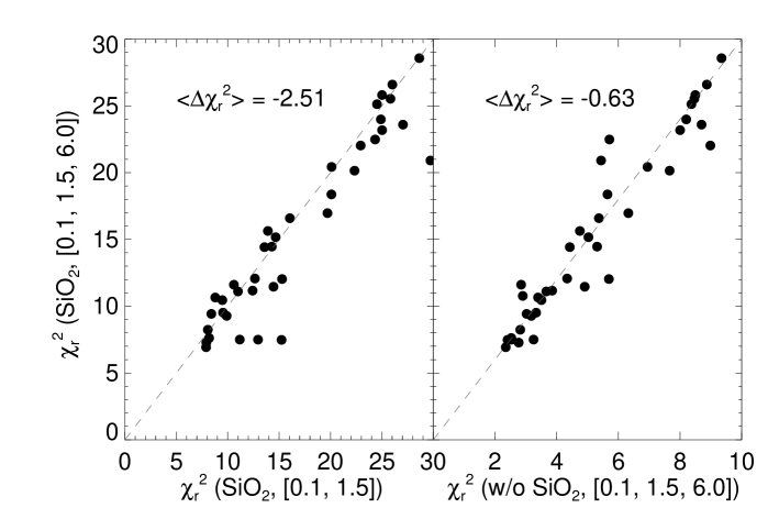
Figure 20: Change in reduced $\chi^{2}_{\mathrm{r}}$ values for fits with and without silica (right panel) and fits with two grain sizes (0.1 and 1.5 $\mu$m, left panel). The dashed line corresponds to $y=x$. The $<\Delta\chi^{2}_{\mathrm{r}}>$ values correspond to the mean difference of reduced $\chi^{2}_{\mathrm{r}}$ between x-axis and y-axis simulations.

Usually, Mg-rich silicates are considered for the dust mineralogy in proto-planetary disks (e.g. Henning & Meeus 2009). But both Olofsson et al. (2009) and Sargent et al. (2009) attribute some features in IRS spectra of young stars to silica (composition SiO₂). To gauge the importance of silica in our B2C compositional approach, we run the B2C model with and without silica. Many fits were improved adding silica in the dust population (as shown for one example in Fig. 21, the 20–22 $\mu$m range being the spectral range where the improvement is the more noticeable). As can be seen on the right panel of Fig. 20, showing the reduced $\chi^{2}_{\mathrm{r}}$ for simulations with and without silica, many fits are improved when silica is included, demonstrating the non-negligible importance of silica for our B2C model.

We have also critically examined the need for large, amorphous, 6.0 $\mu$m-sized grains in the B2C model as they are almost featureless contrary to the 0.1 and 1.5 $\mu$m-sized grains. We therefore run the B2C procedure on the 58 same objects with only 0.1 and 1.5 $\mu$m-sized grains. Left panel of Fig. 20 shows that the mean value of the reduced $\chi^{2}_{\mathrm{r}}$ for all the simulations is augmented by 2.50 when using only two grain sizes, showing that the majority of the fits are improved using three grain sizes instead of two.

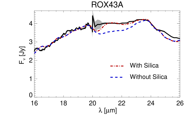
Figure 21: Blowup on the fit to the ROX43A spectrum, performed with silica (red dot-dashed line) and without (blue dashed line).

One can also worry about the influence of the offset $O_{\nu,2}$ values on the inferred grain sizes. As a large offset value leads to larger flux below the continuum–substracted spectrum, it may indeed favor larger grains. We therefore examined if there was any correlation between the fraction of large 6.0 $\mu$m-sized grains and the $O_{\nu,2}$ values, and we quantified these relations with correlation coefficients. Considering the warm large grains and the $O_{\nu,2}$ offsets, we find a $\tau$ value of 0.04 with a significance probability of $P=0.69$. For the cold large grain fraction and the $O_{\nu,2}$ values, we obtain $\tau=-0.03$ and $P=0.70$. This means that there is no significant influence of the offsets $O_{\nu,2}$ on the inferred grain sizes.

Table 3: Dust composition derived using the ”B2C” procedure for 58 objects from our sample. For each star, first line corresponds to the warm component abundances and second line corresponds to the cold component abundances.

	0.1 $\mu$m				1.5 $\mu$m				6.0 $\mu$m
Starname	Am	Ens	For	Sil	Am	Ens	For	Sil	Am	Ens	For	Sil
	%	%	%	%	%	%	%	%	%	%	%	%
AS 205	7.0${}^{+1.4}_{-0.9}$	1.5${}^{+0.8}_{-0.7}$	0.8${}^{+0.7}_{-0.0}$	0.0${}^{+0.3}_{-0.0}$	47.6${}^{+3.0}_{-3.6}$	5.1${}^{+2.0}_{-1.2}$	3.3${}^{+2.0}_{-1.8}$	0.0${}^{+0.6}_{-0.0}$	16.3${}^{+2.2}_{-2.6}$	-	-	18.5${}^{+1.9}_{-2.9}$
…	27.3${}^{+2.1}_{-3.2}$	1.5${}^{+1.0}_{-0.9}$	0.0${}^{+0.7}_{-0.0}$	0.1${}^{+0.7}_{-0.0}$	50.2${}^{+4.5}_{-5.0}$	0.0${}^{+0.9}_{-0.0}$	0.0${}^{+0.9}_{-0.0}$	0.0${}^{+1.3}_{-0.0}$	9.3${}^{+2.5}_{-1.6}$	-	-	11.6${}^{+5.2}_{-3.6}$
B35	32.4${}^{+7.5}_{-7.1}$	0.7${}^{+1.3}_{-0.0}$	0.3${}^{+1.8}_{-0.0}$	0.0${}^{+2.4}_{-0.0}$	54.1${}^{+4.5}_{-4.5}$	0.0${}^{+2.5}_{-0.0}$	0.5${}^{+1.3}_{-0.0}$	0.0${}^{+1.7}_{-0.0}$	8.8${}^{+1.7}_{-0.0}$	-	-	3.3${}^{+1.7}_{-0.0}$
…	23.5${}^{+2.7}_{-2.6}$	0.0${}^{+0.7}_{-0.0}$	0.0${}^{+0.9}_{-0.0}$	0.0${}^{+1.3}_{-0.0}$	50.0${}^{+6.6}_{-11.1}$	3.7${}^{+1.8}_{-2.1}$	0.0${}^{+1.2}_{-0.0}$	0.0${}^{+0.9}_{-0.0}$	5.3${}^{+1.3}_{-1.1}$	-	-	17.5${}^{+4.2}_{-4.5}$
BD+31 634	16.6${}^{+2.2}_{-1.2}$	2.0${}^{+1.5}_{-0.0}$	0.0${}^{+0.4}_{-0.0}$	0.0${}^{+0.6}_{-0.0}$	56.9${}^{+4.6}_{-6.2}$	6.9${}^{+3.6}_{-3.2}$	0.0${}^{+1.3}_{-0.0}$	2.4${}^{+1.5}_{-1.4}$	7.0${}^{+1.5}_{-0.0}$	-	-	8.2${}^{+1.4}_{-2.0}$
…	56.1${}^{+4.3}_{-4.4}$	0.0${}^{+0.8}_{-0.0}$	0.0${}^{+0.7}_{-0.0}$	0.0${}^{+1.3}_{-0.0}$	31.1${}^{+3.0}_{-2.4}$	0.0${}^{+0.6}_{-0.0}$	0.0${}^{+0.6}_{-0.0}$	0.0${}^{+0.6}_{-0.0}$	7.2${}^{+1.2}_{-0.5}$	-	-	5.6${}^{+1.4}_{-0.8}$
C7-11	28.1${}^{+7.8}_{-5.5}$	4.4${}^{+2.3}_{-2.0}$	1.9${}^{+2.9}_{-0.0}$	2.6${}^{+2.6}_{-1.1}$	40.6${}^{+5.2}_{-7.0}$	1.3${}^{+3.2}_{-0.5}$	11.5${}^{+3.4}_{-3.8}$	0.0${}^{+2.4}_{-0.0}$	9.5${}^{+1.4}_{-1.1}$	-	-	0.0${}^{+2.3}_{-0.0}$
…	13.3${}^{+2.5}_{-4.0}$	1.1${}^{+4.5}_{-1.2}$	7.1${}^{+1.8}_{-4.6}$	0.1${}^{+1.2}_{-0.0}$	27.7${}^{+5.0}_{-9.9}$	33.2${}^{+10.1}_{-17.1}$	3.3${}^{+4.5}_{-2.6}$	0.0${}^{+2.7}_{-0.0}$	6.1${}^{+1.5}_{-1.7}$	-	-	8.2${}^{+2.2}_{-3.5}$
CK4	9.4${}^{+9.6}_{-0.0}$	1.8${}^{+1.8}_{-0.0}$	0.0${}^{+2.7}_{-0.0}$	0.0${}^{+0.7}_{-0.0}$	76.3${}^{+5.3}_{-11.0}$	2.7${}^{+5.5}_{-0.0}$	0.0${}^{+4.8}_{-0.0}$	0.0${}^{+1.4}_{-0.0}$	9.7${}^{+3.4}_{-0.0}$	-	-	0.0${}^{+0.7}_{-0.0}$
…	16.3${}^{+1.2}_{-2.8}$	1.8${}^{+0.9}_{-0.9}$	0.0${}^{+1.1}_{-0.0}$	0.0${}^{+0.7}_{-0.0}$	61.2${}^{+4.2}_{-8.4}$	0.0${}^{+1.0}_{-0.0}$	2.1${}^{+1.8}_{-1.0}$	0.0${}^{+1.5}_{-0.0}$	13.0${}^{+2.4}_{-1.6}$	-	-	5.7${}^{+1.6}_{-2.3}$
EC82	35.1${}^{+3.3}_{-2.3}$	5.7${}^{+6.9}_{-0.0}$	0.0${}^{+1.4}_{-0.0}$	0.0${}^{+0.9}_{-0.0}$	26.3${}^{+3.1}_{-1.6}$	16.0${}^{+3.3}_{-1.9}$	6.0${}^{+2.0}_{-0.0}$	0.0${}^{+1.0}_{-0.0}$	0.0${}^{+1.3}_{-0.0}$	-	-	10.8${}^{+2.1}_{-0.0}$
…	38.0${}^{+2.4}_{-1.7}$	0.2${}^{+0.2}_{-0.0}$	0.0${}^{+1.1}_{-0.0}$	0.0${}^{+1.3}_{-0.0}$	45.1${}^{+3.0}_{-2.1}$	0.0${}^{+0.4}_{-0.0}$	0.0${}^{+1.4}_{-0.0}$	0.0${}^{+1.1}_{-0.0}$	16.7${}^{+1.9}_{-2.0}$	-	-	0.0${}^{+1.1}_{-0.0}$
GQ Lup	1.9${}^{+4.0}_{-0.0}$	2.4${}^{+1.4}_{-0.0}$	1.6${}^{+1.3}_{-0.8}$	0.0${}^{+0.5}_{-0.0}$	50.6${}^{+4.9}_{-9.7}$	5.0${}^{+2.8}_{-3.6}$	7.0${}^{+3.9}_{-3.1}$	4.5${}^{+3.5}_{-2.3}$	23.7${}^{+4.8}_{-6.5}$	-	-	3.2${}^{+5.4}_{-0.7}$
…	10.8${}^{+9.4}_{-3.8}$	14.3${}^{+3.7}_{-6.7}$	0.0${}^{+3.5}_{-0.0}$	10.9${}^{+3.8}_{-6.5}$	20.7${}^{+4.4}_{-7.7}$	0.0${}^{+10.7}_{-0.0}$	14.8${}^{+6.2}_{-4.2}$	15.7${}^{+15.0}_{-9.2}$	10.7${}^{+3.6}_{-2.8}$	-	-	2.2${}^{+2.5}_{-1.5}$
GW Lup	7.0${}^{+2.7}_{-1.3}$	2.2${}^{+1.8}_{-0.0}$	0.0${}^{+0.7}_{-0.0}$	0.0${}^{+0.6}_{-0.0}$	24.3${}^{+4.3}_{-7.2}$	7.2${}^{+5.2}_{-2.0}$	7.1${}^{+5.1}_{-3.4}$	0.0${}^{+1.4}_{-0.0}$	52.2${}^{+8.1}_{-4.8}$	-	-	0.0${}^{+6.8}_{-0.0}$
…	0.0${}^{+3.8}_{-0.0}$	27.4${}^{+8.6}_{-8.5}$	0.0${}^{+2.4}_{-0.0}$	0.0${}^{+2.9}_{-0.0}$	0.0${}^{+2.5}_{-0.0}$	0.0${}^{+10.6}_{-0.0}$	17.9${}^{+6.2}_{-4.6}$	2.0${}^{+8.6}_{-0.0}$	52.7${}^{+12.9}_{-12.7}$	-	-	0.0${}^{+8.2}_{-0.0}$
HM 27	63.2${}^{+12.0}_{-10.5}$	3.3${}^{+2.1}_{-2.1}$	2.6${}^{+4.1}_{-0.0}$	0.0${}^{+1.1}_{-0.0}$	18.9${}^{+2.8}_{-0.0}$	1.3${}^{+1.6}_{-0.0}$	5.6${}^{+6.0}_{-1.9}$	0.0${}^{+0.8}_{-0.0}$	5.0${}^{+1.4}_{-0.0}$	-	-	0.0${}^{+0.9}_{-0.0}$
…	26.7${}^{+5.6}_{-5.3}$	0.0${}^{+0.9}_{-0.0}$	0.6${}^{+1.3}_{-0.0}$	0.0${}^{+1.7}_{-0.0}$	52.0${}^{+12.7}_{-8.4}$	7.8${}^{+3.4}_{-2.4}$	0.8${}^{+2.3}_{-0.0}$	2.5${}^{+2.4}_{-1.3}$	4.4${}^{+1.5}_{-0.9}$	-	-	5.2${}^{+1.7}_{-1.1}$
HM Lup	20.7${}^{+7.8}_{-3.4}$	2.4${}^{+1.7}_{-1.3}$	0.5${}^{+2.0}_{-0.0}$	0.0${}^{+1.0}_{-0.0}$	55.3${}^{+13.9}_{-15.2}$	6.6${}^{+4.3}_{-3.3}$	3.7${}^{+4.3}_{-3.0}$	1.1${}^{+2.4}_{-0.0}$	0.0${}^{+3.6}_{-0.0}$	-	-	9.7${}^{+2.6}_{-1.8}$
…	33.5${}^{+10.6}_{-9.7}$	4.0${}^{+3.0}_{-2.3}$	6.2${}^{+4.7}_{-4.1}$	0.0${}^{+2.1}_{-0.0}$	21.9${}^{+6.7}_{-6.1}$	0.4${}^{+2.3}_{-0.0}$	0.0${}^{+2.4}_{-0.0}$	0.0${}^{+1.1}_{-0.0}$	19.5${}^{+6.8}_{-6.5}$	-	-	14.6${}^{+9.5}_{-6.9}$
HT Lup	7.8${}^{+4.8}_{-0.0}$	4.2${}^{+1.8}_{-0.0}$	0.0${}^{+0.8}_{-0.0}$	2.4${}^{+1.4}_{-0.0}$	38.1${}^{+3.7}_{-5.0}$	3.7${}^{+2.7}_{-2.3}$	6.6${}^{+3.3}_{-2.8}$	0.3${}^{+1.3}_{-0.0}$	12.3${}^{+2.7}_{-1.9}$	-	-	24.6${}^{+4.9}_{-2.7}$
…	34.9${}^{+7.0}_{-6.5}$	9.3${}^{+3.3}_{-2.5}$	0.0${}^{+1.0}_{-0.0}$	1.1${}^{+1.7}_{-0.8}$	44.1${}^{+5.9}_{-7.1}$	0.0${}^{+2.2}_{-0.0}$	0.0${}^{+1.9}_{-0.0}$	0.0${}^{+2.3}_{-0.0}$	8.8${}^{+1.5}_{-1.0}$	-	-	1.8${}^{+1.3}_{-0.9}$
Haro 1-1	35.2${}^{+4.0}_{-2.8}$	1.9${}^{+1.7}_{-0.0}$	4.6${}^{+2.3}_{-2.0}$	0.0${}^{+0.5}_{-0.0}$	27.8${}^{+7.0}_{-5.2}$	0.0${}^{+0.8}_{-0.0}$	3.3${}^{+1.8}_{-1.9}$	0.0${}^{+1.6}_{-0.0}$	20.2${}^{+3.4}_{-2.3}$	-	-	6.9${}^{+1.5}_{-2.7}$
…	13.9${}^{+3.3}_{-3.0}$	3.3${}^{+3.4}_{-0.0}$	0.0${}^{+0.8}_{-0.0}$	4.8${}^{+0.9}_{-2.2}$	26.4${}^{+4.7}_{-6.1}$	9.2${}^{+1.9}_{-2.8}$	0.0${}^{+1.1}_{-0.0}$	7.9${}^{+4.2}_{-4.4}$	17.4${}^{+5.2}_{-2.5}$	-	-	17.0${}^{+4.6}_{-6.1}$
Haro 1-16	59.5${}^{+7.1}_{-5.1}$	2.4${}^{+1.4}_{-0.0}$	0.0${}^{+1.7}_{-0.0}$	0.0${}^{+1.8}_{-0.0}$	24.5${}^{+3.2}_{-2.6}$	4.6${}^{+2.4}_{-0.0}$	4.1${}^{+3.3}_{-0.0}$	0.0${}^{+2.8}_{-0.0}$	2.2${}^{+0.7}_{-0.0}$	-	-	2.8${}^{+0.7}_{-0.0}$
…	21.6${}^{+2.2}_{-2.4}$	6.3${}^{+1.0}_{-1.9}$	0.0${}^{+0.6}_{-0.0}$	2.9${}^{+1.5}_{-1.1}$	56.7${}^{+7.0}_{-6.1}$	0.0${}^{+0.6}_{-0.0}$	0.0${}^{+0.6}_{-0.0}$	2.2${}^{+1.5}_{-1.3}$	10.2${}^{+1.0}_{-0.9}$	-	-	0.1${}^{+0.3}_{-0.0}$
Haro 1-17	1.9${}^{+2.1}_{-0.0}$	3.0${}^{+1.1}_{-0.7}$	2.2${}^{+0.9}_{-0.0}$	2.0${}^{+1.0}_{-0.9}$	38.4${}^{+2.9}_{-3.2}$	4.6${}^{+1.8}_{-1.3}$	5.7${}^{+1.9}_{-1.3}$	1.5${}^{+2.1}_{-0.0}$	17.3${}^{+2.9}_{-3.3}$	-	-	23.5${}^{+2.8}_{-4.0}$
…	38.7${}^{+8.8}_{-8.0}$	2.3${}^{+4.2}_{-0.0}$	0.0${}^{+4.9}_{-0.0}$	0.0${}^{+2.4}_{-0.0}$	17.3${}^{+6.3}_{-4.2}$	2.8${}^{+3.6}_{-0.0}$	1.1${}^{+4.9}_{-0.0}$	0.0${}^{+2.4}_{-0.0}$	37.8${}^{+7.2}_{-9.6}$	-	-	0.0${}^{+3.8}_{-0.0}$
Haro 1-4	3.9${}^{+1.5}_{-0.7}$	3.9${}^{+0.9}_{-1.0}$	0.0${}^{+0.5}_{-0.0}$	1.9${}^{+1.4}_{-1.1}$	29.2${}^{+3.1}_{-6.8}$	15.0${}^{+2.7}_{-3.9}$	11.9${}^{+2.2}_{-3.4}$	0.0${}^{+2.3}_{-0.0}$	0.0${}^{+2.0}_{-0.0}$	-	-	34.3${}^{+3.5}_{-11.7}$
…	10.4${}^{+7.3}_{-3.8}$	0.0${}^{+1.6}_{-0.0}$	0.0${}^{+1.6}_{-0.0}$	21.9${}^{+9.0}_{-5.5}$	19.0${}^{+8.1}_{-3.8}$	6.0${}^{+3.4}_{-2.8}$	0.0${}^{+1.1}_{-0.0}$	6.2${}^{+7.0}_{-3.7}$	33.5${}^{+6.0}_{-5.5}$	-	-	3.1${}^{+6.7}_{-1.4}$
Hn 9	1.2${}^{+0.8}_{-0.0}$	1.8${}^{+0.6}_{-0.0}$	0.0${}^{+0.8}_{-0.0}$	0.0${}^{+0.9}_{-0.0}$	53.2${}^{+4.1}_{-9.5}$	4.3${}^{+2.8}_{-2.2}$	4.3${}^{+3.0}_{-1.8}$	0.0${}^{+0.9}_{-0.0}$	23.0${}^{+3.5}_{-3.1}$	-	-	12.2${}^{+2.8}_{-2.4}$
…	15.6${}^{+5.2}_{-0.0}$	1.2${}^{+1.4}_{-0.0}$	0.6${}^{+3.5}_{-0.0}$	0.0${}^{+6.6}_{-0.0}$	45.4${}^{+11.4}_{-7.9}$	0.6${}^{+2.5}_{-0.0}$	0.2${}^{+9.0}_{-0.0}$	0.6${}^{+6.6}_{-0.0}$	30.1${}^{+7.9}_{-5.1}$	-	-	5.7${}^{+7.7}_{-0.0}$
IM Lup	11.9${}^{+3.1}_{-1.3}$	2.9${}^{+1.1}_{-1.1}$	0.5${}^{+1.2}_{-0.0}$	0.0${}^{+0.8}_{-0.0}$	40.2${}^{+5.6}_{-6.0}$	5.2${}^{+3.2}_{-2.9}$	9.9${}^{+2.4}_{-3.3}$	2.0${}^{+2.8}_{-0.0}$	24.0${}^{+2.8}_{-2.6}$	-	-	3.3${}^{+3.4}_{-1.7}$
…	3.5${}^{+5.1}_{-0.0}$	18.8${}^{+10.5}_{-8.8}$	16.3${}^{+9.2}_{-7.7}$	0.0${}^{+4.0}_{-0.0}$	4.3${}^{+9.1}_{-0.0}$	15.2${}^{+10.4}_{-10.3}$	25.1${}^{+14.2}_{-12.6}$	0.0${}^{+5.0}_{-0.0}$	14.1${}^{+6.5}_{-3.5}$	-	-	2.7${}^{+2.9}_{-1.3}$
IRAS 08267-3336	21.4${}^{+3.5}_{-1.7}$	1.1${}^{+1.0}_{-0.0}$	0.1${}^{+1.4}_{-0.0}$	0.0${}^{+0.6}_{-0.0}$	52.9${}^{+4.0}_{-3.0}$	2.8${}^{+1.7}_{-1.5}$	4.5${}^{+2.2}_{-2.0}$	0.0${}^{+1.1}_{-0.0}$	0.4${}^{+1.4}_{-0.0}$	-	-	16.9${}^{+1.5}_{-3.0}$
…	16.6${}^{+3.7}_{-3.9}$	9.9${}^{+2.4}_{-1.7}$	0.0${}^{+0.9}_{-0.0}$	12.8${}^{+2.7}_{-2.5}$	40.3${}^{+5.9}_{-9.2}$	0.0${}^{+1.5}_{-0.0}$	0.0${}^{+2.1}_{-0.0}$	4.1${}^{+2.1}_{-1.7}$	7.7${}^{+1.0}_{-1.1}$	-	-	8.7${}^{+2.3}_{-2.4}$
IRAS 12535-7623	8.5${}^{+2.5}_{-0.8}$	1.4${}^{+1.5}_{-0.0}$	0.0${}^{+0.6}_{-0.0}$	0.3${}^{+0.9}_{-0.0}$	48.8${}^{+3.8}_{-8.3}$	0.8${}^{+2.0}_{-0.0}$	2.0${}^{+2.0}_{-1.2}$	0.0${}^{+1.0}_{-0.0}$	37.3${}^{+2.4}_{-3.5}$	-	-	1.0${}^{+4.1}_{-0.0}$
…	52.2${}^{+5.2}_{-10.2}$	3.3${}^{+2.7}_{-0.0}$	0.0${}^{+1.4}_{-0.0}$	0.0${}^{+1.6}_{-0.0}$	11.4${}^{+1.1}_{-2.3}$	2.0${}^{+1.1}_{-0.9}$	2.3${}^{+1.9}_{-0.0}$	0.0${}^{+0.4}_{-0.0}$	13.3${}^{+4.1}_{-3.2}$	-	-	15.6${}^{+2.5}_{-3.8}$
IRS60	41.4${}^{+6.7}_{-6.0}$	6.2${}^{+2.4}_{-2.5}$	0.0${}^{+1.5}_{-0.0}$	2.4${}^{+2.3}_{-1.5}$	22.5${}^{+3.9}_{-5.8}$	5.7${}^{+2.6}_{-2.3}$	12.9${}^{+2.9}_{-2.8}$	1.1${}^{+1.3}_{-0.6}$	0.0${}^{+1.8}_{-0.0}$	-	-	7.9${}^{+3.2}_{-0.0}$
…	31.0${}^{+3.6}_{-6.9}$	9.0${}^{+6.8}_{-4.6}$	0.0${}^{+2.3}_{-0.0}$	1.0${}^{+4.6}_{-0.0}$	21.1${}^{+2.6}_{-6.2}$	9.3${}^{+2.3}_{-5.9}$	0.0${}^{+5.5}_{-0.0}$	4.7${}^{+2.4}_{-2.7}$	5.8${}^{+1.8}_{-1.2}$	-	-	18.1${}^{+4.0}_{-8.3}$
ISO-ChaII 54	0.0${}^{+0.9}_{-0.0}$	20.6${}^{+3.5}_{-1.9}$	0.0${}^{+5.6}_{-0.0}$	0.0${}^{+0.8}_{-0.0}$	28.3${}^{+4.5}_{-3.6}$	0.0${}^{+1.6}_{-0.0}$	45.7${}^{+5.7}_{-12.0}$	0.0${}^{+1.7}_{-0.0}$	2.1${}^{+1.0}_{-0.0}$	-	-	3.3${}^{+1.6}_{-0.0}$
…	20.0${}^{+3.9}_{-3.5}$	0.0${}^{+2.0}_{-0.0}$	2.6${}^{+2.9}_{-0.0}$	0.0${}^{+0.8}_{-0.0}$	45.1${}^{+13.2}_{-6.8}$	14.5${}^{+7.8}_{-2.7}$	0.0${}^{+2.1}_{-0.0}$	0.0${}^{+2.0}_{-0.0}$	2.8${}^{+2.0}_{-0.0}$	-	-	15.0${}^{+4.7}_{-3.9}$
LkHA 271	17.7${}^{+11.4}_{-2.2}$	3.0${}^{+3.2}_{-1.2}$	0.0${}^{+2.4}_{-0.0}$	0.6${}^{+2.4}_{-0.0}$	37.9${}^{+4.9}_{-10.4}$	7.7${}^{+3.1}_{-3.3}$	0.0${}^{+4.4}_{-0.0}$	0.0${}^{+5.3}_{-0.0}$	25.5${}^{+5.0}_{-5.2}$	-	-	7.5${}^{+7.0}_{-3.2}$
…	37.5${}^{+14.6}_{-12.0}$	0.0${}^{+4.3}_{-0.0}$	4.2${}^{+13.1}_{-0.0}$	17.9${}^{+10.3}_{-7.2}$	15.9${}^{+4.3}_{-3.8}$	0.0${}^{+1.6}_{-0.0}$	2.9${}^{+2.7}_{-2.3}$	2.9${}^{+1.4}_{-2.4}$	6.8${}^{+8.1}_{-2.3}$	-	-	11.8${}^{+6.1}_{-6.6}$
LkHA 326	0.0${}^{+3.3}_{-0.0}$	2.8${}^{+1.4}_{-0.0}$	0.0${}^{+1.1}_{-0.0}$	1.9${}^{+1.2}_{-1.1}$	59.4${}^{+10.2}_{-11.7}$	3.3${}^{+3.8}_{-1.8}$	8.3${}^{+3.8}_{-4.0}$	0.0${}^{+2.3}_{-0.0}$	12.4${}^{+4.4}_{-1.7}$	-	-	11.9${}^{+3.0}_{-3.2}$
…	7.4${}^{+4.1}_{-2.9}$	22.5${}^{+12.9}_{-11.2}$	0.0${}^{+3.2}_{-0.0}$	19.5${}^{+9.5}_{-9.7}$	5.4${}^{+7.6}_{-1.3}$	0.0${}^{+3.5}_{-0.0}$	0.0${}^{+4.2}_{-0.0}$	11.9${}^{+7.2}_{-6.5}$	33.4${}^{+8.6}_{-8.6}$	-	-	0.0${}^{+9.9}_{-0.0}$
LkHA 327	0.0${}^{+3.3}_{-0.0}$	6.6${}^{+2.9}_{-1.4}$	0.0${}^{+0.9}_{-0.0}$	0.1${}^{+1.6}_{-0.0}$	22.5${}^{+8.5}_{-4.0}$	11.8${}^{+2.6}_{-5.8}$	9.6${}^{+5.3}_{-2.2}$	0.0${}^{+3.5}_{-0.0}$	19.1${}^{+12.0}_{-8.5}$	-	-	30.3${}^{+12.2}_{-15.5}$
…	15.1${}^{+4.8}_{-3.1}$	0.0${}^{+0.8}_{-0.0}$	1.3${}^{+2.5}_{-0.0}$	1.7${}^{+2.0}_{-0.9}$	63.9${}^{+16.2}_{-16.6}$	7.7${}^{+6.4}_{-3.3}$	3.4${}^{+3.6}_{-1.8}$	0.0${}^{+3.2}_{-0.0}$	3.1${}^{+3.4}_{-0.0}$	-	-	3.8${}^{+2.5}_{-2.0}$
RNO 90	12.1${}^{+2.6}_{-1.5}$	1.8${}^{+0.6}_{-1.0}$	0.0${}^{+0.6}_{-0.0}$	0.0${}^{+0.9}_{-0.0}$	55.0${}^{+6.8}_{-8.0}$	4.5${}^{+2.8}_{-2.4}$	2.4${}^{+4.0}_{-0.0}$	0.0${}^{+0.9}_{-0.0}$	10.9${}^{+1.4}_{-2.2}$	-	-	13.3${}^{+3.5}_{-2.1}$
…	22.7${}^{+4.1}_{-3.4}$	0.4${}^{+1.8}_{-0.0}$	2.0${}^{+1.7}_{-0.0}$	5.7${}^{+4.1}_{-0.0}$	33.7${}^{+3.4}_{-5.8}$	7.6${}^{+5.7}_{-1.5}$	1.9${}^{+3.5}_{-0.0}$	3.5${}^{+3.5}_{-2.1}$	2.8${}^{+3.4}_{-0.0}$	-	-	19.7${}^{+6.2}_{-7.4}$
ROX42C	20.5${}^{+4.4}_{-4.2}$	8.0${}^{+2.4}_{-2.1}$	3.4${}^{+2.5}_{-2.0}$	13.4${}^{+3.3}_{-2.7}$	28.3${}^{+4.4}_{-6.3}$	0.0${}^{+2.3}_{-0.0}$	10.3${}^{+4.6}_{-2.3}$	0.0${}^{+2.0}_{-0.0}$	7.0${}^{+2.2}_{-1.3}$	-	-	9.1${}^{+3.3}_{-1.6}$
…	14.9${}^{+7.1}_{-7.0}$	8.0${}^{+4.6}_{-4.1}$	48.7${}^{+17.0}_{-12.3}$	0.0${}^{+2.2}_{-0.0}$	6.7${}^{+4.6}_{-3.7}$	0.0${}^{+1.1}_{-0.0}$	9.3${}^{+8.1}_{-6.3}$	0.0${}^{+0.9}_{-0.0}$	12.5${}^{+5.0}_{-4.0}$	-	-	0.0${}^{+5.6}_{-0.0}$
ROX43A	29.7${}^{+3.6}_{-5.3}$	4.8${}^{+2.9}_{-0.0}$	0.0${}^{+1.5}_{-0.0}$	0.0${}^{+1.2}_{-0.0}$	40.0${}^{+4.4}_{-4.7}$	0.0${}^{+0.7}_{-0.0}$	10.7${}^{+2.3}_{-1.5}$	0.7${}^{+1.0}_{-0.0}$	10.9${}^{+2.2}_{-0.0}$	-	-	3.2${}^{+1.2}_{-0.0}$
…	19.1${}^{+5.9}_{-2.7}$	17.4${}^{+4.7}_{-2.7}$	0.0${}^{+0.7}_{-0.0}$	4.9${}^{+3.8}_{-3.4}$	23.5${}^{+3.1}_{-2.3}$	0.0${}^{+0.8}_{-0.0}$	4.4${}^{+1.4}_{-2.0}$	11.1${}^{+3.5}_{-2.1}$	8.2${}^{+2.9}_{-2.5}$	-	-	11.3${}^{+1.9}_{-3.1}$
RU Lup	11.3${}^{+1.6}_{-1.3}$	6.0${}^{+1.2}_{-1.3}$	0.0${}^{+0.3}_{-0.0}$	0.7${}^{+0.5}_{-0.0}$	14.0${}^{+2.1}_{-1.9}$	7.6${}^{+1.4}_{-1.2}$	10.9${}^{+1.5}_{-1.0}$	0.0${}^{+0.6}_{-0.0}$	15.1${}^{+2.8}_{-2.3}$	-	-	34.4${}^{+6.1}_{-4.9}$
…	39.4${}^{+3.1}_{-5.1}$	1.3${}^{+0.9}_{-0.0}$	0.2${}^{+2.1}_{-0.0}$	0.0${}^{+0.6}_{-0.0}$	15.5${}^{+1.3}_{-2.8}$	6.0${}^{+1.3}_{-0.9}$	1.5${}^{+1.5}_{-0.0}$	0.0${}^{+0.4}_{-0.0}$	26.8${}^{+2.3}_{-3.4}$	-	-	9.3${}^{+2.2}_{-1.9}$
RXJ1301.0-7654	30.1${}^{+5.7}_{-4.7}$	1.3${}^{+1.4}_{-0.8}$	0.2${}^{+1.2}_{-0.0}$	0.0${}^{+0.7}_{-0.0}$	40.0${}^{+7.2}_{-8.1}$	3.9${}^{+2.4}_{-2.1}$	2.0${}^{+3.0}_{-0.6}$	0.0${}^{+1.3}_{-0.0}$	13.5${}^{+4.2}_{-2.8}$	-	-	9.0${}^{+1.5}_{-2.1}$
…	9.1${}^{+9.4}_{-4.5}$	8.8${}^{+5.9}_{-4.0}$	5.3${}^{+3.5}_{-3.0}$	0.1${}^{+1.8}_{-0.0}$	23.6${}^{+18.2}_{-6.5}$	4.5${}^{+4.7}_{-2.3}$	16.1${}^{+12.0}_{-8.3}$	0.1${}^{+12.7}_{-0.0}$	28.0${}^{+21.1}_{-11.2}$	-	-	4.4${}^{+11.7}_{-0.0}$
RXJ1615.3-3255	15.0${}^{+3.8}_{-3.1}$	9.5${}^{+2.1}_{-2.8}$	2.1${}^{+5.4}_{-0.0}$	0.0${}^{+1.1}_{-0.0}$	33.0${}^{+4.1}_{-7.8}$	17.3${}^{+4.8}_{-4.3}$	19.8${}^{+4.6}_{-5.2}$	0.1${}^{+2.0}_{-0.0}$	1.7${}^{+4.2}_{-0.0}$	-	-	1.6${}^{+3.0}_{-0.0}$
…	8.7${}^{+9.0}_{-0.0}$	0.0${}^{+3.3}_{-0.0}$	4.0${}^{+10.2}_{-0.0}$	8.4${}^{+18.4}_{-0.0}$	31.7${}^{+26.1}_{-0.0}$	0.1${}^{+4.7}_{-0.0}$	4.8${}^{+13.8}_{-0.0}$	17.6${}^{+35.8}_{-0.0}$	10.8${}^{+11.2}_{-0.0}$	-	-	13.9${}^{+27.4}_{-0.0}$
RY Lup	57.4${}^{+4.6}_{-3.1}$	0.7${}^{+1.9}_{-0.0}$	0.4${}^{+1.1}_{-0.0}$	0.0${}^{+1.5}_{-0.0}$	28.5${}^{+6.2}_{-4.7}$	0.0${}^{+2.8}_{-0.0}$	2.9${}^{+3.3}_{-0.0}$	0.0${}^{+2.9}_{-0.0}$	7.6${}^{+1.7}_{-0.0}$	-	-	2.5${}^{+1.6}_{-0.0}$
…	28.6${}^{+2.7}_{-2.4}$	1.4${}^{+0.9}_{-0.0}$	0.0${}^{+0.9}_{-0.0}$	0.0${}^{+0.7}_{-0.0}$	45.1${}^{+3.9}_{-2.8}$	0.0${}^{+0.5}_{-0.0}$	0.0${}^{+0.5}_{-0.0}$	0.7${}^{+0.5}_{-0.0}$	20.6${}^{+1.9}_{-1.3}$	-	-	3.6${}^{+1.7}_{-1.6}$
SR 9	57.8${}^{+4.2}_{-3.6}$	2.3${}^{+1.3}_{-1.4}$	0.3${}^{+0.7}_{-0.0}$	0.0${}^{+0.4}_{-0.0}$	20.2${}^{+1.7}_{-2.8}$	3.3${}^{+1.9}_{-1.8}$	4.2${}^{+1.3}_{-1.2}$	0.0${}^{+0.7}_{-0.0}$	3.1${}^{+1.6}_{-0.0}$	-	-	8.7${}^{+1.2}_{-1.4}$
…	17.2${}^{+3.9}_{-4.0}$	0.2${}^{+0.7}_{-0.0}$	2.9${}^{+1.0}_{-1.7}$	11.7${}^{+3.0}_{-4.5}$	28.6${}^{+7.9}_{-6.4}$	16.1${}^{+4.9}_{-3.0}$	0.0${}^{+1.6}_{-0.0}$	7.3${}^{+3.3}_{-4.8}$	16.1${}^{+2.4}_{-2.2}$	-	-	0.0${}^{+1.1}_{-0.0}$
SSTc2d J033036.0+303024	14.0${}^{+3.0}_{-1.9}$	4.4${}^{+1.3}_{-1.2}$	0.9${}^{+1.2}_{-0.0}$	2.7${}^{+1.7}_{-1.1}$	49.5${}^{+5.2}_{-7.1}$	0.0${}^{+1.3}_{-0.0}$	11.0${}^{+2.5}_{-1.8}$	0.0${}^{+0.8}_{-0.0}$	11.4${}^{+3.3}_{-1.1}$	-	-	6.1${}^{+1.1}_{-2.1}$
…	26.7${}^{+6.0}_{-5.7}$	14.5${}^{+6.4}_{-6.3}$	11.4${}^{+4.5}_{-4.8}$	0.0${}^{+1.4}_{-0.0}$	24.9${}^{+5.3}_{-3.3}$	8.9${}^{+5.6}_{-5.2}$	0.0${}^{+1.9}_{-0.0}$	0.0${}^{+0.9}_{-0.0}$	12.5${}^{+2.7}_{-2.3}$	-	-	1.1${}^{+2.1}_{-0.0}$
SSTc2d J033037.0+303128	1.8${}^{+2.1}_{-0.0}$	1.6${}^{+1.7}_{-0.0}$	0.0${}^{+1.7}_{-0.0}$	0.0${}^{+0.6}_{-0.0}$	14.8${}^{+7.1}_{-4.1}$	6.8${}^{+3.9}_{-0.0}$	4.9${}^{+3.2}_{-0.0}$	0.0${}^{+2.1}_{-0.0}$	70.1${}^{+13.9}_{-13.0}$	-	-	0.0${}^{+6.7}_{-0.0}$
…	29.5${}^{+6.5}_{-6.0}$	0.4${}^{+1.0}_{-0.0}$	11.9${}^{+4.4}_{-5.7}$	0.0${}^{+0.9}_{-0.0}$	41.2${}^{+6.9}_{-7.2}$	7.1${}^{+2.5}_{-2.0}$	0.2${}^{+2.0}_{-0.0}$	0.0${}^{+1.1}_{-0.0}$	7.9${}^{+1.7}_{-2.3}$	-	-	1.9${}^{+1.9}_{-1.3}$
SSTc2d J033052.5+305418	2.3${}^{+1.4}_{-0.0}$	1.6${}^{+0.8}_{-0.0}$	0.0${}^{+0.6}_{-0.0}$	0.0${}^{+0.6}_{-0.0}$	38.2${}^{+4.8}_{-4.5}$	4.2${}^{+2.5}_{-1.9}$	0.8${}^{+1.3}_{-0.0}$	0.0${}^{+1.0}_{-0.0}$	43.2${}^{+5.6}_{-7.9}$	-	-	9.7${}^{+6.0}_{-2.2}$
…	57.3${}^{+15.8}_{-14.0}$	0.3${}^{+6.3}_{-0.0}$	0.0${}^{+1.8}_{-0.0}$	0.5${}^{+9.6}_{-0.0}$	23.8${}^{+9.2}_{-0.0}$	0.3${}^{+7.9}_{-0.0}$	0.0${}^{+3.6}_{-0.0}$	1.9${}^{+4.9}_{-0.0}$	13.7${}^{+6.7}_{-0.0}$	-	-	2.3${}^{+2.8}_{-0.0}$
SSTc2d J033241.7+311046	3.2${}^{+0.9}_{-0.0}$	1.2${}^{+0.8}_{-0.0}$	0.3${}^{+0.5}_{-0.0}$	0.0${}^{+0.9}_{-0.0}$	26.7${}^{+2.2}_{-2.0}$	2.1${}^{+2.6}_{-0.1}$	3.5${}^{+1.3}_{-1.3}$	0.0${}^{+0.8}_{-0.0}$	56.9${}^{+3.8}_{-11.5}$	-	-	6.1${}^{+4.5}_{-2.6}$
…	59.8${}^{+13.8}_{-11.6}$	0.1${}^{+10.6}_{-0.0}$	0.0${}^{+7.9}_{-0.0}$	0.0${}^{+13.5}_{-0.0}$	22.2${}^{+8.5}_{-0.0}$	1.7${}^{+5.1}_{-0.0}$	0.0${}^{+2.2}_{-0.0}$	1.2${}^{+4.4}_{-0.0}$	3.3${}^{+4.9}_{-0.0}$	-	-	11.8${}^{+10.1}_{-0.0}$
SSTc2d J161159.8-382338	46.0${}^{+11.8}_{-9.0}$	6.2${}^{+1.8}_{-2.8}$	0.0${}^{+2.4}_{-0.0}$	1.6${}^{+3.6}_{-0.0}$	21.5${}^{+4.6}_{-5.9}$	4.1${}^{+3.1}_{-2.0}$	10.2${}^{+3.8}_{-3.5}$	2.1${}^{+2.8}_{-1.2}$	8.3${}^{+4.6}_{-1.2}$	-	-	0.0${}^{+0.9}_{-0.0}$
…	2.4${}^{+18.6}_{-0.7}$	28.0${}^{+14.1}_{-9.0}$	0.0${}^{+5.2}_{-0.0}$	11.8${}^{+7.9}_{-7.9}$	3.0${}^{+6.0}_{-1.7}$	2.3${}^{+9.6}_{-1.0}$	2.0${}^{+10.5}_{-0.0}$	7.0${}^{+3.8}_{-4.4}$	43.4${}^{+8.2}_{-12.1}$	-	-	0.0${}^{+4.3}_{-0.0}$
SSTc2d J162148.5-234027	1.2${}^{+4.8}_{-0.0}$	2.2${}^{+1.7}_{-0.0}$	0.0${}^{+0.9}_{-0.0}$	0.8${}^{+1.8}_{-0.2}$	59.2${}^{+14.2}_{-20.3}$	9.0${}^{+6.9}_{-3.7}$	4.6${}^{+7.1}_{-3.7}$	0.0${}^{+2.9}_{-0.0}$	7.4${}^{+10.1}_{-2.3}$	-	-	15.7${}^{+6.2}_{-8.3}$
…	24.8${}^{+5.2}_{-8.6}$	2.7${}^{+3.4}_{-0.0}$	0.0${}^{+4.9}_{-0.0}$	0.0${}^{+1.9}_{-0.0}$	13.1${}^{+3.9}_{-4.8}$	0.0${}^{+1.1}_{-0.0}$	5.8${}^{+2.2}_{-4.2}$	0.1${}^{+7.3}_{-0.6}$	29.0${}^{+7.1}_{-7.6}$	-	-	24.5${}^{+9.9}_{-12.9}$
SSTc2d J162245.4-243124	10.2${}^{+3.8}_{-1.8}$	2.0${}^{+2.2}_{-0.0}$	0.0${}^{+1.1}_{-0.0}$	1.9${}^{+1.4}_{-0.0}$	73.1${}^{+8.0}_{-8.6}$	6.2${}^{+6.4}_{-1.9}$	0.0${}^{+1.6}_{-0.0}$	0.0${}^{+1.4}_{-0.0}$	6.6${}^{+3.0}_{-0.0}$	-	-	0.0${}^{+0.3}_{-0.0}$
…	46.5${}^{+12.2}_{-8.5}$	0.0${}^{+2.5}_{-0.0}$	0.0${}^{+1.8}_{-0.0}$	1.3${}^{+3.8}_{-0.0}$	11.4${}^{+5.8}_{-3.2}$	27.9${}^{+16.9}_{-13.6}$	0.0${}^{+2.9}_{-0.0}$	0.0${}^{+2.8}_{-1.8}$	10.5${}^{+4.5}_{-3.9}$	-	-	2.5${}^{+0.8}_{-1.4}$
SSTc2d J162715.1-245139	54.9${}^{+7.4}_{-6.5}$	3.6${}^{+1.7}_{-2.1}$	0.0${}^{+1.5}_{-0.0}$	0.0${}^{+1.1}_{-0.0}$	22.2${}^{+3.1}_{-6.8}$	5.2${}^{+2.3}_{-1.9}$	4.2${}^{+3.3}_{-2.4}$	0.0${}^{+1.0}_{-0.0}$	6.2${}^{+2.1}_{-0.7}$	-	-	3.7${}^{+2.9}_{-0.0}$
…	4.5${}^{+3.3}_{-0.0}$	5.0${}^{+5.4}_{-0.8}$	37.4${}^{+21.2}_{-18.1}$	6.3${}^{+5.7}_{-0.0}$	7.3${}^{+4.3}_{-0.0}$	8.0${}^{+5.3}_{-0.0}$	4.4${}^{+3.4}_{-2.2}$	0.0${}^{+2.4}_{-0.0}$	27.2${}^{+12.3}_{-9.6}$	-	-	0.0${}^{+3.4}_{-0.0}$
SSTc2d J162816.7-240514	0.0${}^{+1.6}_{-0.0}$	16.7${}^{+2.6}_{-1.5}$	0.0${}^{+1.6}_{-0.0}$	3.6${}^{+1.4}_{-1.3}$	25.8${}^{+5.3}_{-6.6}$	0.8${}^{+2.0}_{-0.0}$	12.0${}^{+1.8}_{-4.4}$	0.0${}^{+0.9}_{-0.0}$	41.2${}^{+3.2}_{-7.8}$	-	-	0.0${}^{+5.8}_{-0.0}$
…	21.2${}^{+5.5}_{-2.9}$	2.3${}^{+2.3}_{-0.0}$	0.1${}^{+1.5}_{-0.0}$	0.0${}^{+1.0}_{-0.0}$	55.9${}^{+11.1}_{-8.2}$	2.9${}^{+2.6}_{-2.2}$	0.0${}^{+2.3}_{-0.0}$	0.0${}^{+4.2}_{-0.0}$	12.9${}^{+4.4}_{-2.0}$	-	-	4.7${}^{+5.4}_{-0.0}$
SSTc2d J182850.2+00950	7.2${}^{+4.6}_{-0.0}$	0.6${}^{+0.9}_{-0.0}$	0.8${}^{+0.8}_{-0.0}$	0.0${}^{+0.4}_{-0.0}$	63.9${}^{+5.5}_{-13.0}$	3.6${}^{+2.8}_{-2.0}$	1.9${}^{+2.9}_{-0.9}$	0.0${}^{+1.1}_{-0.0}$	5.5${}^{+3.4}_{-0.3}$	-	-	16.6${}^{+2.1}_{-3.3}$
…	48.5${}^{+11.2}_{-10.6}$	9.9${}^{+3.0}_{-4.6}$	0.0${}^{+2.8}_{-0.0}$	5.1${}^{+3.4}_{-2.7}$	5.6${}^{+1.3}_{-1.4}$	4.2${}^{+2.4}_{-2.5}$	0.3${}^{+2.2}_{-0.0}$	6.9${}^{+1.8}_{-3.0}$	13.6${}^{+2.7}_{-3.0}$	-	-	5.8${}^{+1.5}_{-3.3}$
SSTc2d J182900.9+02931	0.6${}^{+3.4}_{-0.0}$	1.2${}^{+1.0}_{-0.0}$	0.0${}^{+0.5}_{-0.0}$	2.4${}^{+0.7}_{-0.7}$	69.9${}^{+7.4}_{-9.7}$	8.4${}^{+3.9}_{-3.7}$	3.7${}^{+3.0}_{-2.3}$	0.0${}^{+1.5}_{-0.0}$	6.6${}^{+4.7}_{-2.5}$	-	-	7.2${}^{+4.7}_{-0.0}$
…	8.6${}^{+2.3}_{-4.9}$	9.9${}^{+6.4}_{-5.0}$	8.8${}^{+3.9}_{-6.5}$	0.3${}^{+1.7}_{-0.0}$	12.0${}^{+4.9}_{-2.7}$	28.3${}^{+15.0}_{-18.1}$	1.7${}^{+2.5}_{-1.4}$	0.1${}^{+1.8}_{-0.0}$	12.4${}^{+4.9}_{-3.6}$	-	-	17.9${}^{+6.2}_{-13.8}$
SSTc2d J182909.8+03446	2.0${}^{+0.6}_{-0.0}$	0.0${}^{+0.6}_{-0.0}$	0.0${}^{+1.1}_{-0.0}$	2.0${}^{+0.6}_{-0.0}$	67.3${}^{+4.3}_{-2.7}$	5.6${}^{+1.4}_{-1.7}$	0.0${}^{+1.0}_{-0.0}$	0.0${}^{+0.6}_{-0.0}$	7.7${}^{+1.7}_{-0.8}$	-	-	15.4${}^{+1.7}_{-2.3}$
…	21.4${}^{+2.6}_{-2.1}$	0.0${}^{+0.4}_{-0.0}$	0.0${}^{+0.8}_{-0.0}$	6.0${}^{+3.2}_{-2.5}$	55.1${}^{+5.8}_{-6.8}$	4.1${}^{+1.9}_{-2.0}$	0.0${}^{+0.8}_{-0.0}$	3.9${}^{+1.3}_{-2.7}$	6.9${}^{+0.8}_{-0.7}$	-	-	2.5${}^{+0.7}_{-0.6}$
SX Cha	19.7${}^{+4.1}_{-4.8}$	3.1${}^{+2.4}_{-0.0}$	0.2${}^{+1.4}_{-0.0}$	0.0${}^{+0.7}_{-0.0}$	44.3${}^{+9.8}_{-7.1}$	6.5${}^{+3.8}_{-3.4}$	4.9${}^{+3.7}_{-2.5}$	0.0${}^{+2.1}_{-0.0}$	11.2${}^{+2.4}_{-3.0}$	-	-	10.1${}^{+3.1}_{-2.7}$
…	20.1${}^{+4.2}_{-4.2}$	0.0${}^{+2.0}_{-0.0}$	0.0${}^{+1.9}_{-0.0}$	0.0${}^{+0.8}_{-0.0}$	28.0${}^{+4.4}_{-6.3}$	6.0${}^{+2.8}_{-2.3}$	0.0${}^{+0.9}_{-0.0}$	0.0${}^{+1.6}_{-0.0}$	10.1${}^{+4.1}_{-2.1}$	-	-	35.9${}^{+11.3}_{-11.7}$
Sz102	18.4${}^{+7.3}_{-0.0}$	1.3${}^{+3.5}_{-0.0}$	0.0${}^{+3.9}_{-0.0}$	0.0${}^{+4.3}_{-0.0}$	68.6${}^{+10.5}_{-11.6}$	4.1${}^{+4.0}_{-0.0}$	0.1${}^{+3.4}_{-0.0}$	0.0${}^{+4.7}_{-0.0}$	2.0${}^{+1.1}_{-0.0}$	-	-	5.4${}^{+1.9}_{-0.0}$
…	24.6${}^{+3.6}_{-3.0}$	1.3${}^{+1.1}_{-0.0}$	0.0${}^{+0.8}_{-0.0}$	0.0${}^{+0.7}_{-0.0}$	58.6${}^{+6.6}_{-6.1}$	0.0${}^{+0.8}_{-0.0}$	3.5${}^{+1.5}_{-1.5}$	0.0${}^{+0.9}_{-0.0}$	5.3${}^{+1.2}_{-0.9}$	-	-	6.8${}^{+2.1}_{-1.3}$
Sz50	64.1${}^{+10.9}_{-18.6}$	4.5${}^{+3.1}_{-2.7}$	1.7${}^{+4.5}_{-1.2}$	2.3${}^{+4.6}_{-0.0}$	5.5${}^{+2.5}_{-1.2}$	10.0${}^{+2.3}_{-2.9}$	8.9${}^{+1.9}_{-3.4}$	0.0${}^{+1.3}_{-0.0}$	0.0${}^{+1.8}_{-0.0}$	-	-	3.0${}^{+3.6}_{-0.0}$
…	25.6${}^{+515.7}_{-0.0}$	0.0${}^{+56.8}_{-0.0}$	4.5${}^{+163.4}_{-0.0}$	1.7${}^{+89.9}_{-0.0}$	8.3${}^{+141.2}_{-0.0}$	13.0${}^{+426.3}_{-0.0}$	0.0${}^{+63.2}_{-0.0}$	9.9${}^{+320.1}_{-0.0}$	19.7${}^{+338.9}_{-0.0}$	-	-	17.3${}^{+551.4}_{-0.0}$
Sz52	1.5${}^{+2.6}_{-0.7}$	2.4${}^{+1.1}_{-0.0}$	0.0${}^{+0.6}_{-0.0}$	1.2${}^{+1.1}_{-0.5}$	52.8${}^{+17.6}_{-12.4}$	5.9${}^{+4.8}_{-4.4}$	7.0${}^{+3.6}_{-4.3}$	0.7${}^{+5.0}_{-0.0}$	10.0${}^{+5.7}_{-4.9}$	-	-	18.4${}^{+7.4}_{-12.3}$
…	23.6${}^{+9.4}_{-9.3}$	16.9${}^{+8.5}_{-8.2}$	2.1${}^{+8.0}_{-3.2}$	0.0${}^{+6.0}_{-0.6}$	42.6${}^{+14.0}_{-14.6}$	0.0${}^{+10.1}_{-0.0}$	0.0${}^{+6.5}_{-0.0}$	0.0${}^{+3.6}_{-0.0}$	13.3${}^{+4.5}_{-4.4}$	-	-	1.6${}^{+1.7}_{-1.3}$
Sz62	0.0${}^{+3.4}_{-0.0}$	3.9${}^{+1.2}_{-0.8}$	0.0${}^{+1.1}_{-0.0}$	5.2${}^{+1.7}_{-1.3}$	24.1${}^{+4.1}_{-4.6}$	7.3${}^{+3.4}_{-4.2}$	19.3${}^{+3.5}_{-5.1}$	0.6${}^{+3.3}_{-0.0}$	36.0${}^{+3.9}_{-8.2}$	-	-	3.6${}^{+2.9}_{-3.0}$
…	9.9${}^{+5.2}_{-2.0}$	0.0${}^{+2.3}_{-0.0}$	6.3${}^{+4.8}_{-3.9}$	0.2${}^{+6.5}_{-0.3}$	58.5${}^{+22.0}_{-14.8}$	10.8${}^{+14.4}_{-4.3}$	0.0${}^{+6.3}_{-0.0}$	0.6${}^{+6.5}_{-0.0}$	3.9${}^{+9.1}_{-0.0}$	-	-	9.8${}^{+4.4}_{-3.5}$
Sz73	12.1${}^{+3.1}_{-1.6}$	2.4${}^{+1.2}_{-0.0}$	0.0${}^{+1.3}_{-0.0}$	0.0${}^{+1.1}_{-0.0}$	46.2${}^{+10.0}_{-9.9}$	3.2${}^{+2.1}_{-1.6}$	4.3${}^{+3.1}_{-2.4}$	0.0${}^{+1.4}_{-0.0}$	25.2${}^{+3.1}_{-4.8}$	-	-	6.6${}^{+5.0}_{-2.7}$
…	10.4${}^{+2.2}_{-2.0}$	5.5${}^{+3.9}_{-3.0}$	0.0${}^{+1.0}_{-0.0}$	3.2${}^{+2.1}_{-2.2}$	44.7${}^{+5.2}_{-7.6}$	7.9${}^{+2.5}_{-3.5}$	0.0${}^{+1.4}_{-0.0}$	4.7${}^{+3.1}_{-2.5}$	11.3${}^{+4.0}_{-1.7}$	-	-	12.3${}^{+4.0}_{-4.2}$
Sz76	6.1${}^{+2.2}_{-0.7}$	0.7${}^{+1.1}_{-0.0}$	0.0${}^{+0.4}_{-0.0}$	0.5${}^{+1.0}_{-0.0}$	27.9${}^{+7.3}_{-7.2}$	7.9${}^{+2.4}_{-2.4}$	0.0${}^{+1.5}_{-0.0}$	0.0${}^{+1.6}_{-0.0}$	38.8${}^{+6.9}_{-7.4}$	-	-	18.2${}^{+9.0}_{-4.3}$
…	16.9${}^{+11.5}_{-0.0}$	3.7${}^{+3.6}_{-0.0}$	0.0${}^{+1.3}_{-0.0}$	14.3${}^{+8.2}_{-7.8}$	6.6${}^{+7.3}_{-0.0}$	0.0${}^{+2.3}_{-0.0}$	1.5${}^{+1.8}_{-0.0}$	17.2${}^{+5.4}_{-9.4}$	19.0${}^{+4.8}_{-4.4}$	-	-	20.8${}^{+8.9}_{-7.6}$
Sz96	37.2${}^{+3.6}_{-2.7}$	4.6${}^{+1.2}_{-2.4}$	2.1${}^{+1.8}_{-1.2}$	0.0${}^{+1.0}_{-0.0}$	38.4${}^{+6.0}_{-7.1}$	0.0${}^{+1.1}_{-0.0}$	8.7${}^{+1.8}_{-3.1}$	0.0${}^{+0.9}_{-0.0}$	1.3${}^{+1.1}_{-0.0}$	-	-	7.8${}^{+1.5}_{-0.0}$
…	24.5${}^{+4.4}_{-3.0}$	15.3${}^{+3.2}_{-2.1}$	3.1${}^{+1.7}_{-1.3}$	0.8${}^{+1.6}_{-0.0}$	23.8${}^{+3.3}_{-2.8}$	5.6${}^{+1.9}_{-1.5}$	2.3${}^{+3.3}_{-0.0}$	1.0${}^{+1.6}_{-0.0}$	23.6${}^{+2.8}_{-1.9}$	-	-	0.0${}^{+1.4}_{-0.0}$
TW Cha	66.7${}^{+12.0}_{-6.3}$	2.7${}^{+4.2}_{-0.0}$	0.0${}^{+4.1}_{-0.0}$	0.0${}^{+1.1}_{-0.0}$	11.0${}^{+2.6}_{-0.0}$	5.8${}^{+3.8}_{-4.0}$	8.1${}^{+3.5}_{-0.0}$	0.4${}^{+3.7}_{-0.0}$	3.6${}^{+5.1}_{-0.0}$	-	-	1.6${}^{+5.4}_{-0.0}$
…	14.1${}^{+1.1}_{-1.9}$	2.2${}^{+1.2}_{-1.1}$	0.0${}^{+0.4}_{-0.0}$	0.0${}^{+0.7}_{-0.0}$	68.0${}^{+4.8}_{-8.9}$	1.1${}^{+1.7}_{-0.7}$	0.0${}^{+1.0}_{-0.0}$	1.8${}^{+2.4}_{-0.0}$	7.8${}^{+0.8}_{-1.8}$	-	-	4.9${}^{+0.9}_{-1.3}$
V710 Tau	14.8${}^{+3.9}_{-3.0}$	3.7${}^{+2.4}_{-0.9}$	0.0${}^{+2.6}_{-0.0}$	1.1${}^{+2.3}_{-0.0}$	17.9${}^{+4.2}_{-3.8}$	8.4${}^{+3.1}_{-3.1}$	18.2${}^{+3.1}_{-3.3}$	2.3${}^{+2.6}_{-1.4}$	21.4${}^{+6.1}_{-5.6}$	-	-	12.2${}^{+2.3}_{-3.4}$
…	10.1${}^{+7.3}_{-2.1}$	16.9${}^{+18.1}_{-4.9}$	0.0${}^{+2.1}_{-0.0}$	1.6${}^{+2.9}_{-0.0}$	0.0${}^{+3.4}_{-0.0}$	13.3${}^{+15.2}_{-4.4}$	22.0${}^{+23.5}_{-7.0}$	10.6${}^{+12.4}_{-4.0}$	13.9${}^{+7.9}_{-2.3}$	-	-	11.7${}^{+13.7}_{-4.8}$
VW Cha	4.6${}^{+2.0}_{-0.6}$	2.3${}^{+1.2}_{-0.0}$	0.3${}^{+0.4}_{-0.1}$	0.0${}^{+0.3}_{-0.0}$	28.6${}^{+4.1}_{-3.9}$	3.2${}^{+1.9}_{-1.8}$	4.7${}^{+2.0}_{-1.6}$	0.6${}^{+0.8}_{-0.0}$	43.4${}^{+6.5}_{-7.2}$	-	-	12.3${}^{+2.4}_{-3.9}$
…	8.9${}^{+130.1}_{-0.0}$	10.5${}^{+83.5}_{-0.0}$	4.7${}^{+46.6}_{-0.0}$	6.1${}^{+54.3}_{-0.0}$	23.8${}^{+232.1}_{-0.0}$	0.0${}^{+94.4}_{-0.0}$	13.6${}^{+112.3}_{-0.0}$	13.3${}^{+132.8}_{-0.0}$	11.8${}^{+108.7}_{-0.0}$	-	-	7.3${}^{+116.2}_{-0.0}$
VZ Cha	7.7${}^{+5.9}_{-1.9}$	2.4${}^{+1.8}_{-0.8}$	2.6${}^{+3.3}_{-0.7}$	0.0${}^{+1.1}_{-0.0}$	55.0${}^{+9.9}_{-18.3}$	8.1${}^{+4.9}_{-4.1}$	8.0${}^{+5.2}_{-3.7}$	1.7${}^{+3.1}_{-0.8}$	3.8${}^{+5.9}_{-0.2}$	-	-	10.7${}^{+2.7}_{-2.5}$
…	3.7${}^{+12.2}_{-0.9}$	11.3${}^{+3.4}_{-11.8}$	0.0${}^{+4.4}_{-0.0}$	18.0${}^{+19.5}_{-6.9}$	18.8${}^{+15.8}_{-5.2}$	0.0${}^{+16.2}_{-0.0}$	13.4${}^{+16.4}_{-3.8}$	3.1${}^{+5.1}_{-0.7}$	25.6${}^{+13.0}_{-4.6}$	-	-	6.3${}^{+14.9}_{-2.0}$
WX Cha	1.6${}^{+2.6}_{-0.0}$	1.7${}^{+0.8}_{-0.0}$	0.0${}^{+0.7}_{-0.0}$	1.6${}^{+1.9}_{-0.0}$	56.1${}^{+8.6}_{-9.8}$	3.8${}^{+2.6}_{-2.5}$	2.9${}^{+2.6}_{-1.7}$	0.7${}^{+1.6}_{-0.0}$	23.7${}^{+4.4}_{-5.0}$	-	-	7.8${}^{+3.5}_{-2.2}$
…	19.6${}^{+6.2}_{-4.6}$	7.8${}^{+3.8}_{-3.9}$	0.0${}^{+3.9}_{-0.0}$	8.0${}^{+3.3}_{-5.4}$	32.5${}^{+7.6}_{-7.8}$	0.0${}^{+7.1}_{-0.0}$	5.6${}^{+4.3}_{-3.0}$	9.9${}^{+4.7}_{-5.4}$	11.0${}^{+3.1}_{-3.0}$	-	-	5.7${}^{+4.3}_{-2.9}$
XX Cha	16.6${}^{+5.7}_{-3.0}$	2.4${}^{+2.2}_{-1.4}$	0.0${}^{+4.1}_{-0.0}$	2.7${}^{+4.8}_{-0.6}$	22.0${}^{+8.2}_{-7.0}$	14.2${}^{+9.6}_{-3.6}$	11.5${}^{+11.6}_{-4.0}$	7.6${}^{+10.8}_{-3.8}$	3.2${}^{+10.8}_{-0.0}$	-	-	19.8${}^{+7.2}_{-13.7}$
…	13.9${}^{+11.3}_{-8.9}$	0.0${}^{+5.7}_{-0.0}$	12.0${}^{+10.3}_{-10.5}$	11.4${}^{+3.7}_{-9.1}$	12.3${}^{+13.0}_{-6.0}$	11.9${}^{+9.5}_{-9.7}$	26.0${}^{+15.3}_{-16.7}$	0.5${}^{+7.6}_{-0.0}$	11.9${}^{+5.5}_{-5.2}$	-	-	0.0${}^{+3.1}_{-0.0}$

Table 3: continued.

Table 4: Dust temperatures, continuum parameters (blackbody temperature and offset $O_{\nu,2}$) derived using the ”B2C” procedure for 60 objects from our sample.

	Dust temperatures		Continuum		Goodness
Starname	$T_{\mathrm{warm}}$	$T_{\mathrm{cold}}$	$T_{\mathrm{cont}}$	$O_{\nu,2}$	$\chi^{2}_{\mathrm{r}}$	Dof
	(K)	(K)	(K)	($\times$ 100)	-	-
AS 205	228.9${}^{+2.7}_{-2.1}$	58.2${}^{+1.3}_{-0.9}$	121.6${}^{+1.2}_{-1.8}$	20.1${}^{+0.3}_{-0.5}$	22.6	1119
B35	207.3${}^{+5.0}_{-3.7}$	79.5${}^{+1.7}_{-0.0}$	97.4${}^{+3.0}_{-1.1}$	16.0${}^{+0.7}_{-0.8}$	16.9	232
BD+31 634	596.2${}^{+27.1}_{-16.2}$	98.3${}^{+2.3}_{-2.6}$	107.6${}^{+0.9}_{-0.7}$	6.9${}^{+0.3}_{-0.2}$	61.0	231
C7-11	188.2${}^{+2.9}_{-1.8}$	75.2${}^{+4.9}_{-1.1}$	95.1${}^{+0.9}_{-1.2}$	6.1${}^{+0.3}_{-0.1}$	15.9	238
CK4	238.0${}^{+9.3}_{-8.5}$	80.9${}^{+1.3}_{-0.8}$	79.3${}^{+1.3}_{-0.9}$	12.9${}^{+0.2}_{-0.1}$	25.6	1151
EC82	491.6${}^{+25.7}_{-19.9}$	88.8${}^{+1.8}_{-1.0}$	72.0${}^{+3.4}_{-0.0}$	27.3${}^{+0.5}_{-0.4}$	157.7	1159
GQ Lup	192.8${}^{+2.5}_{-1.6}$	70.7${}^{+2.2}_{-3.7}$	85.2${}^{+0.7}_{-0.5}$	12.9${}^{+0.2}_{-0.1}$	23.8	611
GW Lup	341.4${}^{+10.7}_{-13.1}$	102.9${}^{+3.7}_{-5.5}$	119.9${}^{+1.6}_{-1.3}$	8.4${}^{+0.2}_{-0.3}$	46.3	639
HM 27	252.6${}^{+14.6}_{-8.2}$	91.0${}^{+2.9}_{-3.0}$	65.8${}^{+1.3}_{-6.2}$	9.9${}^{+0.0}_{-0.0}$	10.6	236
HM Lup	226.9${}^{+6.2}_{-5.2}$	99.4${}^{+12.9}_{-0.0}$	106.9${}^{+0.8}_{-1.4}$	13.8${}^{+0.5}_{-0.6}$	8.4	235
HT Lup	226.0${}^{+4.9}_{-3.8}$	87.1${}^{+1.9}_{-1.9}$	94.0${}^{+1.3}_{-0.9}$	12.6${}^{+0.2}_{-0.2}$	39.6	1136
Haro 1-1	224.1${}^{+4.1}_{-5.7}$	85.2${}^{+2.6}_{-2.1}$	83.5${}^{+0.6}_{-0.4}$	41.9${}^{+0.7}_{-0.4}$	21.0	643
Haro 1-16	231.8${}^{+4.9}_{-4.5}$	85.6${}^{+2.1}_{-2.2}$	81.8${}^{+0.8}_{-0.5}$	41.5${}^{+0.6}_{-0.4}$	32.6	237
Haro 1-17	188.4${}^{+1.7}_{-1.2}$	60.3${}^{+2.3}_{-3.9}$	95.6${}^{+1.5}_{-2.1}$	24.7${}^{+0.3}_{-0.4}$	37.5	643
Haro 1-4	184.9${}^{+1.8}_{-2.4}$	53.1${}^{+1.6}_{-1.6}$	90.8${}^{+1.7}_{-1.3}$	29.7${}^{+0.8}_{-0.8}$	31.0	1247
Hn 9	211.8${}^{+5.6}_{-3.0}$	65.2${}^{+1.9}_{-5.1}$	112.5${}^{+4.4}_{-5.0}$	24.6${}^{+0.8}_{-0.9}$	9.0	235
IM Lup	225.9${}^{+3.1}_{-2.2}$	107.3${}^{+4.2}_{-4.1}$	104.0${}^{+0.8}_{-0.7}$	15.1${}^{+0.3}_{-0.3}$	34.9	717
IRAS 08267-3336	194.1${}^{+3.0}_{-1.8}$	83.4${}^{+2.6}_{-2.1}$	88.9${}^{+0.6}_{-0.4}$	32.9${}^{+0.4}_{-0.3}$	34.3	643
IRAS 12535-7623	208.2${}^{+2.0}_{-1.4}$	74.0${}^{+2.5}_{-2.0}$	142.3${}^{+5.2}_{-24.8}$	30.7${}^{+0.8}_{-1.4}$	11.4	229
IRS60	183.5${}^{+2.8}_{-1.8}$	82.3${}^{+4.0}_{-2.4}$	88.5${}^{+0.6}_{-0.5}$	13.6${}^{+0.3}_{-0.1}$	25.3	636
ISO-ChaII 54	118.6${}^{+1.3}_{-1.1}$	48.9${}^{+1.2}_{-1.2}$	123.2${}^{+1.4}_{-0.9}$	4.5${}^{+0.1}_{-0.3}$	92.8	211
LkHA 271	182.6${}^{+4.3}_{-3.7}$	55.6${}^{+1.5}_{-3.1}$	96.2${}^{+3.5}_{-2.9}$	12.0${}^{+0.3}_{-0.6}$	14.5	1136
LkHA 326	184.4${}^{+3.6}_{-2.5}$	92.3${}^{+3.5}_{-3.6}$	89.0${}^{+0.6}_{-0.4}$	8.1${}^{+0.3}_{-0.2}$	17.1	643
LkHA 327	201.9${}^{+4.9}_{-8.7}$	67.6${}^{+1.9}_{-1.6}$	150.0${}^{+4.4}_{-4.3}$	3.5${}^{+0.4}_{-0.3}$	18.4	1136
RNO 90	216.1${}^{+2.0}_{-1.5}$	59.7${}^{+1.3}_{-1.2}$	117.5${}^{+0.9}_{-1.6}$	16.2${}^{+0.5}_{-0.3}$	22.2	636
ROX42C	219.1${}^{+4.2}_{-6.3}$	103.0${}^{+2.3}_{-3.3}$	114.4${}^{+0.8}_{-0.6}$	6.9${}^{+0.5}_{-0.3}$	40.9	230
ROX43A	221.9${}^{+3.9}_{-3.1}$	80.8${}^{+1.7}_{-1.9}$	104.7${}^{+2.8}_{-1.6}$	33.6${}^{+0.6}_{-0.4}$	152.1	654
RU Lup	205.1${}^{+2.6}_{-1.6}$	60.6${}^{+1.1}_{-1.2}$	128.7${}^{+1.7}_{-1.0}$	21.0${}^{+0.7}_{-0.5}$	44.0	636
RXJ1301.0-7654	227.9${}^{+6.1}_{-5.1}$	101.0${}^{+2.8}_{-4.2}$	122.1${}^{+1.9}_{-1.9}$	19.1${}^{+0.9}_{-0.5}$	7.0	235
RXJ1615.3-3255	207.8${}^{+3.7}_{-2.7}$	13.1${}^{+1.5}_{-0.0}$	89.0${}^{+0.6}_{-0.4}$	15.5${}^{+0.4}_{-0.3}$	15.4	228
RY Lup	244.0${}^{+7.1}_{-4.6}$	73.5${}^{+2.1}_{-1.2}$	76.1${}^{+4.6}_{-0.0}$	43.3${}^{+1.1}_{-0.7}$	51.8	636
SR 9	203.2${}^{+2.2}_{-3.0}$	91.4${}^{+3.5}_{-1.6}$	95.2${}^{+0.8}_{-0.5}$	35.2${}^{+0.6}_{-0.5}$	29.1	248
SSTc2d J033036.0+303024	190.0${}^{+1.5}_{-2.7}$	76.6${}^{+1.9}_{-3.9}$	94.5${}^{+1.8}_{-1.6}$	30.9${}^{+0.6}_{-0.4}$	46.6	246
SSTc2d J033037.0+303128	329.4${}^{+10.9}_{-19.1}$	96.8${}^{+3.2}_{-3.0}$	99.0${}^{+1.5}_{-5.5}$	15.2${}^{+0.2}_{-0.1}$	31.7	261
SSTc2d J033052.5+305418	217.7${}^{+3.2}_{-3.5}$	61.6${}^{+1.6}_{-3.8}$	150.0${}^{+2.9}_{-2.2}$	33.7${}^{+1.1}_{-2.7}$	7.6	228
SSTc2d J033241.7+311046	227.2${}^{+3.7}_{-2.7}$	60.2${}^{+2.0}_{-2.1}$	150.0${}^{+0.5}_{-3.5}$	31.2${}^{+1.5}_{-3.8}$	11.0	228
SSTc2d J161159.8-382338	220.2${}^{+6.0}_{-5.9}$	58.6${}^{+2.5}_{-3.1}$	117.4${}^{+1.9}_{-1.8}$	10.2${}^{+0.6}_{-0.5}$	11.3	236
SSTc2d J162148.5-234027	207.1${}^{+6.6}_{-6.2}$	38.1${}^{+2.2}_{-0.7}$	100.4${}^{+1.0}_{-0.8}$	14.6${}^{+0.6}_{-0.3}$	7.7	259
SSTc2d J162245.4-243124	202.3${}^{+4.3}_{-2.9}$	90.3${}^{+2.3}_{-4.6}$	107.8${}^{+0.9}_{-0.6}$	17.9${}^{+0.7}_{-0.6}$	37.1	247
SSTc2d J162715.1-245139	182.8${}^{+3.6}_{-2.9}$	101.5${}^{+10.0}_{-1.4}$	99.8${}^{+0.7}_{-0.6}$	21.2${}^{+0.8}_{-1.2}$	14.7	221
SSTc2d J162816.7-240514	162.2${}^{+2.1}_{-2.8}$	59.0${}^{+1.6}_{-2.3}$	142.2${}^{+4.4}_{-4.6}$	10.9${}^{+0.3}_{-1.3}$	26.2	239
SSTc2d J182850.2+00950	206.8${}^{+2.8}_{-2.4}$	83.8${}^{+4.3}_{-1.6}$	80.5${}^{+0.7}_{-0.7}$	22.7${}^{+0.2}_{-0.2}$	7.6	221
SSTc2d J182900.9+02931	232.8${}^{+4.1}_{-3.6}$	38.3${}^{+4.7}_{-0.0}$	112.4${}^{+0.9}_{-1.2}$	4.4${}^{+0.2}_{-0.1}$	24.4	241
SSTc2d J182909.8+03446	220.8${}^{+2.1}_{-1.4}$	70.3${}^{+1.8}_{-1.1}$	90.5${}^{+3.9}_{-1.0}$	35.2${}^{+0.4}_{-0.3}$	54.4	241
SX Cha	268.4${}^{+8.4}_{-6.4}$	80.2${}^{+2.3}_{-1.4}$	97.7${}^{+1.7}_{-1.2}$	15.2${}^{+0.8}_{-0.6}$	23.3	1233
Sz102	195.6${}^{+6.4}_{-4.4}$	80.3${}^{+1.3}_{-0.8}$	85.9${}^{+1.1}_{-0.7}$	25.9${}^{+0.9}_{-0.6}$	26.7	1244
Sz50	164.6${}^{+3.0}_{-1.2}$	66.8${}^{+44.6}_{-0.0}$	85.3${}^{+0.7}_{-0.4}$	4.6${}^{+0.1}_{-0.1}$	9.6	253
Sz52	280.8${}^{+7.5}_{-10.6}$	44.0${}^{+2.3}_{-0.6}$	122.5${}^{+2.4}_{-2.1}$	6.2${}^{+0.2}_{-0.5}$	9.4	269
Sz62	215.6${}^{+3.3}_{-3.1}$	58.4${}^{+2.4}_{-2.8}$	150.0${}^{+0.5}_{-4.8}$	10.7${}^{+0.5}_{-1.3}$	12.3	235
Sz73	196.0${}^{+3.6}_{-3.1}$	87.9${}^{+2.3}_{-1.8}$	96.4${}^{+0.8}_{-0.6}$	11.4${}^{+0.4}_{-0.3}$	28.8	636
Sz76	299.1${}^{+9.2}_{-5.0}$	44.8${}^{+1.4}_{-1.5}$	111.6${}^{+1.1}_{-0.8}$	19.1${}^{+0.9}_{-0.7}$	7.6	228
Sz96	226.7${}^{+3.6}_{-2.7}$	86.0${}^{+1.6}_{-1.5}$	88.0${}^{+0.7}_{-1.3}$	31.9${}^{+0.3}_{-0.4}$	20.8	253
TW Cha	260.3${}^{+8.8}_{-9.2}$	91.2${}^{+1.6}_{-1.0}$	72.0${}^{+0.8}_{-0.5}$	34.7${}^{+0.3}_{-0.2}$	10.8	218
V710 Tau	234.3${}^{+4.3}_{-3.9}$	19.0${}^{+1.8}_{-1.1}$	100.5${}^{+0.7}_{-0.5}$	10.0${}^{+0.2}_{-0.2}$	20.5	221
VW Cha	209.0${}^{+2.2}_{-1.7}$	71.6${}^{+2.3}_{-13.0}$	93.4${}^{+0.8}_{-0.6}$	31.2${}^{+0.5}_{-0.3}$	12.2	232
VZ Cha	233.6${}^{+5.7}_{-3.7}$	38.6${}^{+1.3}_{-1.8}$	139.4${}^{+3.9}_{-3.0}$	6.4${}^{+0.3}_{-0.2}$	9.7	233
WX Cha	239.5${}^{+3.4}_{-2.5}$	82.5${}^{+2.6}_{-2.8}$	100.4${}^{+1.0}_{-1.5}$	21.3${}^{+0.5}_{-0.4}$	11.6	244
XX Cha	223.3${}^{+10.8}_{-10.8}$	102.2${}^{+4.7}_{-8.1}$	99.9${}^{+0.9}_{-0.9}$	8.6${}^{+0.3}_{-0.5}$	7.4	245

Table 4: continued.