Exchange and correlation effects in the transmission phase through a few-electron quantum dot

Abstract

The transmission phase through a quantum dot with few electrons shows a complex, non-universal behavior. Here we combine configuration-interaction calculations —treating rigorously Coulomb interaction— and the Friedel sum rule to provide a rationale for the experimental findings. The phase evolution for more than two electrons is found to strongly depend on dot’s shape and electron density, whereas from one to two the phase never lapses. In the Coulomb (Kondo) regime the phase shifts are significant fractions of $\pi$ ($\pi/2$) for the second and subsequent charge addition if the dot is strongly correlated. These results are explained by the proper inclusion in the theory of Coulomb interaction, spin, and orbital degrees of freedom.

I Introduction

Recent experiments by the Weizmann group have stirred much attention to the phase that electrons acquire when they traverse a quantum dot (QD) embedded in the arm of a Aharonov-Bohm interferometer.Moty ; Zaffalon These fascinating measurements call for a deeper understanding of electron transport through a strongly interacting object. If many electrons — say $N>10$ — populate a QD, the transmission phase $\Theta$ of the tunneling electron displays a much studiedSchuster97 ; Hackenbroich01 universal behavior: first $\Theta$ increases by $\pi$ through the conductance peak and then it lapses in the Coulomb valley. Here we focus on the relatively less studied few-electron regime, where the phase evolution depends on $N$. In the samples studied in Ref. Moty, the phase remains constant in the $N=1$ valley, independently from QD tunings, whereas it lapses in the Coulomb blockaded devices of Ref. Zaffalon, . For $N>2$ the phase is not reproducible and shows both increments and lapses, likely due to QD shape and exchange effects.Moty

In spite of several explanations of the few-electron scenarioMoty ; Karrasch07 ; Hecht09 ; Meden05 ; Golosov06 ; Entin-Wohlman00 ; Bertoni07 ; Silvestrov07 ; Gurvitz07 ; Yahalom06 ; Baksmaty08 a clear picture is still missing. Many works introduced major simplifications, like spinless electrons,Karrasch07 ; Meden05 ; Golosov06 one-dimensional QDs,Entin-Wohlman00 ; Bertoni07 simplified models for Coulomb interaction,Karrasch07 ; Silvestrov07 ; Gurvitz07 ; Hecht09 or other ad hoc assumptions.Yahalom06 Even the interpretation of the simplest $N=1\rightarrow N=2$ transition is controversial, being variably attributed to the occupation of either the sameZaffalon or a differentMoty orbital from that of the first electron, to the role of excited doorway channels,Baksmaty08 to electron crystallization.Gurvitz07

In this paper we compute $\Theta$ by fully including exchange and correlation effects. The theory is based on the application of the Friedel sum rule (FSR) as generalized in Ref. RontaniFSR, to a multiorbital interacting QD—an exact zero-temperature result, $T=0$. Since the FSR holds for non degenerate ground states (GSs) only,RontaniFSR ; Langreth66 it may be applied to either singlet Kondo GSs at zero field, $B=0$, or non-degenerate GSs in the Coulomb blockade regime ($B\geq 0$ for singlets and $B>0$ for doublets and higher-spin states).

It is worth recalling that, in the conductance valleys with odd $N$ at $T=0$ and $B=0$, the QD is always in the Kondo regime. In order to reach the Coulomb blockade regime by keeping $T=0$, one needs to apply the field to the Aharonov-Bohm ring to destroy dot-lead Kondo correlations, hence removing QD spin degeneracy.Ng88 This condition is reached when $\Gamma\ll\mu_{B}B$, with $\mu_{\text{B}}$ being the Bohr magneton and $\Gamma$ the QD level width. In the experiments the temperature is very low ($T\sim 30$ mK) and the field is relatively weak ($B\sim 10$ mT). Therefore, in order to compare measurements with the theoretical predictions reported in this paper, tiny widths $\Gamma$ are required, which are actually smaller than the values presently reported.Moty ; Zaffalon

As anticipated above, the theory relies on the application of the FSR. The key idea is that the phase variation $\Delta\Theta$ for the addition of one electron to the QD is given by integrating the QD spectral density ${\cal N}(\omega)$ between two consecutive conductance valleys (with $\Delta N=1$). This is evaluated exactly for an isolated QD via full configuration interaction (CI) calculationsRontani06 with $N\leq 5$.

The simulations agree with the Coulomb-blockade results of Ref. Moty, : (i) The phase evolution for $2\leq N\leq 5$ strongly depends on the dot’s shape and density. (ii) $\Theta$ never lapses in the $N=1$ valley, independently from dot parameters. Additionaly, (iii) in the Coulomb (Kondo) regime the increment $\Delta\Theta$ through the conductance peak is significantly smaller than $\pi$ ($\pi/2$) as a consequence of strong Coulomb correlation.

The theory fails to reproduce the Coulomb blockade results of Ref. Zaffalon, . The reason of this discrepancy is presently unclear, but it is likely related to the significant departure from the condition ruling the range of applicability of the theory, i.e., $\Gamma\ll\mu_{B}B$ at $T=0$. In order to treat the Coulomb blockade regime even at $B=0$, one could compute the thermal Green function of the fully correlated system at $T>T_{K}$, with $T_{K}$ being the Kondo temperature. We leave for future work this alternative route, which would immediately provide the transmission phase $\Theta$ without invoking the FSR.RontaniFSR

The structure of this paper is as follows. In Sec. II we set the theoretical model and illustrate the usage of the FSR to compute the transmission phase variation $\Delta\Theta$ between consecutive conductance valleys. After briefly recalling the full CI method in Sec. III, we address in Sec. IV the evolution of the phase in the absence of Coulomb interaction (but taking into account the spin degree of freedom). We eventually consider the fully interacting case in Sec. V.

II Transmission phase from the Friedel sum rule

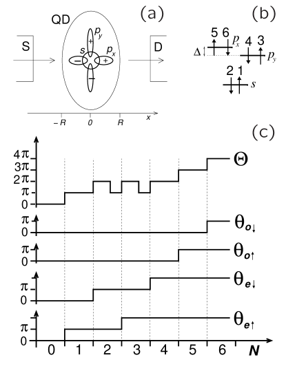
Figure 1: (a) Experimental setup. (b) QD single-particle levels for $a/b<1$. The number sequence points to the consecutive filling of six electrons in a non-interacting picture. (c) Transmission phase $\Theta$ and phase shifts $\Delta\theta_{X\sigma}$ vs $N$ for the filling sequence plotted in (b).

We model the experimental setup of Ref. Moty, as in Fig. 1(a). Electrons flow along $x$ from source (S) to drain (D), tunneling through a QD of elliptical shape. The ellipse is the generic low-energy form for a two-dimensional shallow, gate-defined potential,Moty ; Zaffalon since the lowest-order non-vanishing terms of its series expansion are quadratic. The scattering matrix $S_{\sigma}$ is diagonal in the spin index $\sigma$ in both Kondo and Coulomb blockade regimes. In fact, in the Kondo regime ($B=0$), no elastic spin-flip occurs.Langreth66 ; Ng88 On the other hand, in the Coulomb blockade regime only one $\sigma$ channel is active at time for a given energy since $B$ removes spin degeneracy.

Additionaly, we assumeNoteSymmetry mirror reflection symmetry in the $yz$ plane placed in the QD center, at $x=0$ [Fig. 1(a)], hence the stationary scattering states $\psi_{\sigma}(x)$, eigenstates of $S_{\sigma}$, are either even ($e$) or odd ($o$) with respect to $x\rightarrow-x$ reflection: for $\left|x\right|>R$,

$$\psi_{e\sigma}(x)=e^{-ik\left|x\right|}+e^{2i\theta_{e\sigma}}e^{ik\left|x\right|}$$

and

$$\psi_{o\sigma}(x)=\text{sgn}(x)\left[e^{-ik\left|x\right|}+e^{2i\theta_{o\sigma}}e^{ik\left|x\right|}\right].$$

Here the even and odd outgoing waves are phase shifted by $\theta_{e\sigma}$ and $\theta_{o\sigma}$, respectively, $k$ is the wave vector, $R$ is the QD nominal longitudinal axis. The left and right travelling states $\psi_{\pm k\sigma}(x)$ are superpositions of even and odd states:

$$\psi_{\pm k\sigma}(x)=\frac{1}{2}\left[\psi_{e\sigma}(x)\mp\psi_{o\sigma}(x)\right].$$

Inside the QD, $\left|x\right|<R$, electrons experience two-body Coulomb interactions in addition to the confinement potential [cf. Eq. (4)].

We first generalize the results of Ref. Lee99, for spinless, non interacting electrons by including spins. The transmission amplitude $t_{\sigma}$ for travelling states $\psi_{\pm k\sigma}(x)$ is:

$$t_{\sigma}=\left|t_{\sigma}\right|ie^{i\Theta}=ie^{i\left(\theta_{e\sigma}+\theta_{o\sigma}\right)}\sin{\left(\theta_{e\sigma}-\theta_{o\sigma}\right)}.$$ (1)

Each time $\sin{\left(\theta_{e\sigma}-\theta_{o\sigma}\right)}$ appearing in Eq. (1) changes sign, due to a variation of either $\theta_{e\sigma}$ or $\theta_{o\sigma}$ as a new electron tunnels into the QD, then a lapse of $\pi$ occurs for the transmission phase $\Theta$. Since this happens when $t_{\sigma}=0$ [cf. Eq. (1)], the lapse is located in the conductance valley.Lee99 ; Taniguchi99

We then include all many-body correlations by connecting the phase shift $\theta_{X\sigma}$ per channel $(X,\sigma)$ ($X=e,o$ labels the parity) to the exact spectral density ${\mathcal{N}}_{X\sigma}(\omega)$ accumulated at the QD via the FSR [cf. Eq. (20) of Ref. RontaniFSR, ]:

$$\frac{1}{\hbar}\frac{d\,\theta_{X\sigma}(\omega)}{d\omega}=\pi{\mathcal{N}}_{X\sigma}(\omega).$$ (2)

Here ${\mathcal{N}}_{X\sigma}(\omega)$ is the density displaced at the QD by the electron in the scattering state $(X,\sigma)$ tunneling at the energy $\hbar\omega$ fixed by the chemical potential $\mu=\hbar\omega$. We mimic the action of the plunger gate in the linear response regime by varying the value of $\mu$ with respect to the QD energy levels.

In practice, to use the FSR we integrate it over the energy window between two consecutive Coulomb valleys with $N$ and $N+1$ electrons in the QD, respectively.notaFSR Whereas this procedure provides the information on the total phase variation only, $\Delta\theta_{X\sigma}=\pi\,\Delta{\mathcal{N}}_{X\sigma}=\pi\hbar\int d\omega{\mathcal{N}}_{X\sigma}(\omega)$, it allows to compute $\Delta{\mathcal{N}}_{X\sigma}$ from the interacting Hamiltonian of the isolated dot, $H_{\text{QD}}$. This key result is based on the conservation of the total number of scattering plus QD states both in the presence and absence of the QD in the arm of the interferometer.RontaniFSR

The CI evaluation of $\Delta\theta_{X\sigma}$ relies on the formula

$$\Delta{\mathcal{N}}_{X\sigma}=\frac{\Delta\theta_{X\sigma}}{\pi}=\sum_{\alpha_{X}}\left|\left<\Psi_{0}^{N+1}|c^{\dagger}_{\alpha_{X}\sigma}|\Psi_{0}^{N}\right>\right|^{2},$$ (3)

where $\left|\Psi_{0}^{N}\right>$ is the exact interacting GS of the isolated QD with $N$ electrons of energy $E_{0}^{N}$, $H_{\text{QD}}\left|\Psi_{0}^{N}\right>=E_{0}^{N}\left|\Psi_{0}^{N}\right>$, and $c^{\dagger}_{\alpha_{X}\sigma}$ creates an electron with spin $\sigma$ in the orbital of given parity $X$ and further specified by the set of quantum numbers $\alpha_{X}$. Equation (3) follows from Eq. (21) of Ref. RontaniFSR, , which was inferred by connecting the phase shift to the delay time spent by the electron wave packet in the QD. This delay is obtained by integrating the wave function square modulus over both time and space. By orthogonality of QD orbitals, only terms diagonal in $\alpha_{X}$ indices survive in the formula (3).

We eventually link the transmission phase variation $\Delta\Theta$ to $\Delta\theta_{X\sigma}$ through Eq. (1). In the Coulomb blockade regime only one scattering channel $(X,\sigma)$ is active at time between two consecutive valleys with respectively $N$ and $N+1$ electrons. The active channel is univocally determined by the total spins and parities of $\left|\Psi_{0}^{N}\right>$ and $\left|\Psi_{0}^{N+1}\right>$, as obtained by CI. On the other hand, in the Kondo regime time-reversal invariance (recall that $B=0$) implies that $\Delta{\mathcal{N}}_{X\uparrow}=\Delta{\mathcal{N}}_{X\downarrow}$, evaluated as half the Coulomb blockade value given by Eq. (3). In this way we regain at once the resultZaffalon ; Langreth66 that $\Delta\Theta=\pi/2$ for the addition of the first electron. In fact, the term on the right hand side of Eq. (3) is trivially one when $N=0$.

III The full configuration interaction method

The interacting Hamiltonian of the isolated QD is

$$H_{\text{QD}}=\sum_{i=1}^{N}H_{\text{SP}}(i)+\frac{1}{2}\sum_{i\neq j}\frac{e^{2}}{\kappa|\bm{r}_{i}-\bm{r}_{j}|},$$ (4)

where the single particle (SP) term is

$$H_{\text{SP}}(i)=\frac{\bm{p}_{i}^{2}}{2m^{*}}+\frac{1}{2}m^{*}\!\left(\omega_{0x}^{2}x_{i}^{2}+\omega_{0y}^{2}y_{i}^{2}\right)+\frac{1}{2}g^{*}\sigma_{i}\,\mu_{B}B.$$ (5)

Here $\sigma_{i}=\pm 1$, $\kappa$ is the dielectric constant, $m^{*}$ is the electron effective mass, $g^{*}$ is the gyromagnetic factor, and the QD confinement frequencies in the $x$ and $y$ directions, $\omega_{0x}$ and $\omega_{0y}$, have characteristic lengths $a=[\hbar/(m^{*}\omega_{0x})]^{1/2}$ and $b=[\hbar/(m^{*}\omega_{0y})]^{1/2}$, respectively (the ratio $a/b$ is related to the ellipse eccentrity). In Eq. (4) the weak $B$ does not affect orbital degrees of freedom.

To wholly include in our theory Coulomb correlation, we solve numerically the few-body problem of Eq. (4) by means of the full CI method (also known as exact diagonalization, for details see Ref. Rontani06, ). The CI few-body GS $\left|\Psi_{0}^{N}\right>$ is essentially a linear combination of the Slater determinants $\left|\Phi_{i}^{N}\right>$,

$$\left|\Psi_{0}^{N}\right>=\sum_{i}c_{i}\left|\Phi_{i}^{N}\right>,$$ (6)

with the unknown $c_{i}$s being the output of the calculation. Here the determinants $\left|\Phi_{i}^{N}\right>$ are obtained by filling in all possible ways with $N$ electrons the $N_{\text{SP}}$ lowest-energy SP orbitals (two-fold spin degenerate at $B=0$), eigenstates of the SP Hamiltonian (5). In the Fock space of these Slater determinants $H_{\text{QD}}$ is a large sparse matrix, that we exactly diagonalize by means of the parallel code DonRodrigo,website eventually obtaining the coefficients $c_{i}$ of Eq. (6).

The diagonalization proceeds in each Hilbert space sector labeled by $N$, the total spin, and the total parity of the few-body wave function. After we have obtained the GSs $\left|\Psi_{0}^{N}\right>$ and $\left|\Psi_{0}^{N+1}\right>$, we evaluate $\Delta{\mathcal{N}}_{X\sigma}$ via Eq. (3), and eventually infer $\Delta\Theta$ as explained in Sec. II.

In the CI calculations reported in Sec. V we used $N_{\text{SP}}=36$ and diagonalized matrices of maximum linear size 2.25 $\times 10^{6}$. The relative error for the energy was less than $10^{-4}$ for $a/b=1$.

IV The spinful non-interacting case

To illustrate the effect of the inclusion of the spin degree of freedom in the calculation of the transmission phase $\Theta$ let us consider for the time being only the SP Hamiltonian, $H_{\text{SP}}$, and neglect Coulomb interaction. The GS is a Slater determinant with the lowest $N$ spin-orbitals filled, $\left|\Psi^{N}_{0}\right>=\prod_{i=1}^{N}c^{\dagger}_{\alpha_{i}\sigma_{i}}\!\left|0\right>$ ($\left|0\right>$ is the vacuum). The Aufbau filling sequence for $1\leq N\leq 6$ is depicted in Fig. 1(b) for $a/b<1$. The first two electrons occupy the $s$ orbital with opposite spin, then the 3rd and 4th electrons fill in the $p_{y}$ orbital, which is shifted in energy from the $p_{x}$ orbital by $\Delta=\hbar\omega_{0x}(1-a^{2}/b^{2})$. Note that the first electron entering a new SP level is always $\uparrow$, due to the effect of $B$. The evaluation of the phase shift $\Delta\theta_{X\sigma}$ at each electron addition is straightforward, since in Eq. (3) only one addendum gives a non-zero contribution to $\Delta\theta_{X\sigma}/\pi$ —exactly one— as a new spin-orbital $(\alpha_{X},\sigma)$ is occupied; the other ones vanish due to the orthogonality of the states. Therefore in Fig. 1(b) one has $\Delta{\mathcal{N}}_{X\sigma}=1$ for the sequence $(X,\sigma)=(e,\uparrow)$, $(e,\downarrow)$, $(e,\uparrow)$, $(e,\downarrow)$, $(o,\uparrow)$, $(o,\downarrow)$ of six consecutive electron additions, with the $p_{y}$ ($p_{x}$) orbital even (odd) under $x\rightarrow-x$.

The evolution of $\Theta$ for the filling sequence of Fig. 1(b) is shown in Fig. 1(c). Both increments and lapses of $\Theta$ are derived through Eq. (1) (lapse locations in the conductance valleys with fixed $N$ are arbitrary). A remarkable feature of Fig. 1(c) is that $\Theta$ increases by $\pi$ in both transitions $N=0\rightarrow N=1$ and $N=1\rightarrow N=2$, since the first two electrons occupy the same $s$ orbital with opposite spin. This is fundamentally different from the spinless case,Lee99 where a total increase of $\Theta$ by $2\pi$ between $N=0$ and $N=2$ occurs only if the two electrons occupy orbitals of different parities.

Two lapses of $\pi$ occur for $\Theta$ in the blockaded regions with $N=2$ and $N=3$ [Fig. 1(c)] as the phases $\theta_{e\uparrow}$ and $\theta_{e\downarrow}$ increase more than $\pi$, respectively. The whole pattern of $\Theta$ in Fig. 1(c) up to five electrons coincides with Fig. 4a of Ref. Moty, , provided that one interprets the $N=3\rightarrow N=4$ smooth transition as a phase lapse (in Sec. V we consider an alternative interpretation). This agreement is surprising, since in the experiment SP levels have a small energy separation ($\sim 0.5$ meV), if compared to characteristic Coulomb energies ($\sim 1-3$ meV),Moty and therefore one would expect significant differences from the non-interacting model of Fig. 1. On the other hand, the $\Theta$-evolution would be basically the same as in Fig. 1 if the interacting QD ground state were well approximated by a single Slater determinant, as in Hartee-Fock theory where Coulomb interaction is included as a mean field.

V The role of Coulomb interaction

When correlation effects beyond the mean-field levelexplanation are relevant, we expect that $\Delta{\mathcal{N}}_{X\sigma}<1$, as suggested in Ref. RontaniFSR, . Since the CI ground states $\left|\Psi_{0}^{N}\right>$ are superpositions of the Slater determinants $\left|\Phi_{i}^{N}\right>$ [cf. Eq. (6)], after expansion on this basis many cross terms give no contribution to Eq. (3): the stronger the correlation, the larger the number of Slater determinants, the smaller $\Delta{\mathcal{N}}_{X\sigma}$. This seems to be the case in Ref. Moty, for $\Delta\Theta\sim 3\pi/4$ in the $N=1\rightarrow N=2$ transition of Fig. 4b and $\Delta\Theta\sim 3\pi/4$ for $N=6\rightarrow N=7$ in Fig. 5. This could even be the case for $\Delta\Theta\sim 0$ for $N=3\rightarrow N=4$ in Fig. 4a of Ref. Moty, , if one excludes the possibility of a phase lapse. Such interpretation is alternative to the one suggested in the previous section.

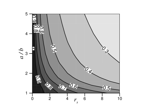
Figure 2: Contour plot of $\Delta\Theta$ in the $(r_{s},\,a/b)$ space, in units of $\pi$, for the $N=1\rightarrow N=2$ transition in the Coulomb blockade regime. The grey code goes from 0 (white) to 1 (black). The value in the Kondo regime is obtained by dividing $\Delta\Theta$ by two.

To assess the impact of correlation in the CI results, we parameterize the electron density $n$ of the circular dot ($\omega_{0}=\omega_{0x}=\omega_{0y}$) via the dimensionless radius $r_{s}$ of the circle whose area is equal to the area per electron, $r_{s}=1/[a_{\text{B}}^{*}(\pi n)^{1/2}]$, where $a_{\text{B}}^{*}$ is the effective Bohr radius and $n$ is estimated as in Ref. Garcia05, . We next focus on the evolution of $\Theta$ as a function of both $r_{s}$ and ellipse anisotropy ratio $a/b$. The first electron addition in the Coulomb (Kondo) regime always gives $\Delta\Theta=\pi$ ($\Delta\Theta=\pi/2$). Then $\Theta$ remains constant in the $N=1$ valley, independently from the values of either $r_{s}$ or $a/b$ [cf. Fig. 3]. The second electron addition is analyzed in Fig. 2, plotting in the $(r_{s},\,a/b)$ space the contour map of $\Delta\Theta$ for $N=1\rightarrow N=2$. Here we vary the anisotropy ratio $a/b$ by keeping the ellipse area $\pi ab$ fixed, so the density remains constant. The contour lines of Fig. 2 provide the value of $\Delta\Theta$ in the Coulomb blockade regime, whereas its Kondo counterpart may be simply obtained by dividing $\Delta\Theta$ by two (cf. also Fig. 3). As $r_{s}$ increases, $\Delta\Theta$ monotonously decreases, since correlation effects become stronger at lower density, as the Coulomb term in $H_{\text{QD}}$ [Eq. (4)] overcomes the SP term. A similar trend occurs by increasing $a/b$, since a stronger anisotropy effectively lowers the dimensionality of the system, again enforcing correlation effects.notaCN Note that by overlapping the experimental value $\Delta\Theta\sim 3\pi/4$ with the plot of Fig. 2 we find $r_{s}\approx 4$ for $a/b=1$. This value corresponds to $\hbar\omega_{0}=1.2$ meV for GaAs, which is comparable to the experimental estimate of 0.5 meV.Moty

From the analysis of CI data of Fig. 2 we find that the orbital parities of both the first and second electrons are always even, independently from $r_{s}$ and $a/b$. This prediction agrees with the Wigner-Mattis theorem: the two-electron GS is always a singlet and the orbital part of its wave function is nodeless.Mattis65 This result conflicts with other explanations,Moty ; Baksmaty08 and it is expected to hold even in the presence of disorder and/or more complicated potentials.

Figure 3: $\Theta$ vs $N$ for different dot anisotropies $a/b$. Solid (dashed) lines refer to the Coulomb blockade (Kondo) regime. We used GaAs parameters and $\hbar\omega_{0}=0.5$ meV. From top to bottom: $a/b=$ (1.5)^-1, (1.15)^-1, (1.05)^-1, 1, 1.05, 1.15, 1.5.

In Fig. 3 we follow the evolution of $\Theta$ up to five electrons for a significant range of QD anisotropies. At the experimental density ($\hbar\omega_{0}=0.5$ meV) a slight variation of $a/b$ is sufficient to alter the phase behavior for $N>2$. Indeed, the relative differences between the values of $a/b$ for the 3rd, 4th, and 5th panels are as small as 5%. Therefore, $\Theta$ is sensitive to fluctuations of the experimental QD parameters, as reported in Ref. Moty, .

The occurrence of alternative scenarios in Fig. 3 is another signature of correlation. In fact, several excited states lie very close in energy to the GS, as it is the case in the crossover to electron crystallization.Reimann02 ; Kalliakos08 ; Singha10 Hence a small deformation of the QD shape easily induces a crossing between states of different symmetry. We here highlight only the most relevant features of a rich zoology, focusing on Coulomb blockade results (solid lines in Fig. 3). In a circular QD at such low density (4th panel of Fig. 3) the three-electron GS is a spin quadruplet as an effect of correlation.Rontani06 Because the two-electron GS is a singlet, the transition $N=2\rightarrow N=3$ is spin blockaded, i.e., $\Delta\Theta=0$ without any lapse as $\Delta{\mathcal{N}}_{X\sigma}=0$. A slight deformation of the QD (3rd and 5th panels) changes the $N=3$ GS into a doublet, lifting the spin blockade ($\Delta\Theta\neq 0$ between $N=2$ and $N=3$). The $N=4$ GS is a more robust triplet, since the spin polarization is due to Hund’s rule —an open shell effect.Reimann02 However, a stronger deformation of the QD (2nd and 6th panels) breaks the orbital degeneracy of the SP levels of the 2nd shell inducing a transition to a singlet GS. At such anisotropy ratios singlets and doublets typically alternate for even and odd electron numbers, respectively. A further increase of the deformation (1st and 7th panels) changes the filling sequence of higher-energy orbitals.

In Fig. 3 we also plot $\Theta$ in the Kondo regime (dashed lines) for those cases such that the QD spin is totally screened by the cloud of opposite-spin tunneling electrons.Hewson This excludes high-spin GSs other than singlets an doublets occuring in the 3rd, 4th, and 5th panels. The hallmark of correlation is that $\Delta\Theta$ is a fraction of $\pi$ and $\pi/2$ in the Coulomb blockade and Kondo regimes, respectively [e.g., compare the SP phase evolution of Fig. 1(c) with its correlated counterpart in the 2nd panel of Fig. 3].

VI Conclusion

In conclusion, we highlighted the role of exchange and correlation in the transmission phase of a few-electron quantum dot. Our findings are relevant for transport experiments through strongly interacting nano objects, including molecules and carbon-based nanostructures.

- (1) M. Avinum-Kalish, M. Heiblum, O. Zarchin, D. Mahalu, and V. Umansky, Nature (London) 436, 529 (2005).
- (2) M. Zaffalon, A. Bid, M. Heiblum, D. Mahalu, and V. Umansky, Phys. Rev. Lett. 100, 226601 (2008).
- (3) R. Schuster, E. Buks, M. Heiblum, D. Mahalu, V. Umansky, and H. Shtrikman, Nature (London) 385, 417 (1997).
- (4) G. Hackenbroich, Phys. Rep. 343, 463 (2001).
- (5) C. Karrasch, T. Hecht, A. Weichselbaum, Y. Oreg, J. von Delft, and V. Meden, Phys. Rev. Lett. 98, 186802 (2007).
- (6) T. Hecht, A. Weichselbaum, Y. Oreg, and J. von Delft, Phys. Rev. B 80, 115330 (2009).
- (7) V. Meden and F. Marquardt, Phys. Rev. Lett. 96, 146801 (2006).
- (8) D. I. Golosov and Y. Gefen, Phys. Rev. B 74, 205316 (2006).
- (9) O. Entin-Wohlman, A. Aharony, Y. Imry, and Y. Levinson, Europhys. Lett. 50, 354 (2000).
- (10) A. Bertoni and G. Goldoni, Phys. Rev. B 75, 235318 (2007).
- (11) P. G. Silvestrov and Y. Imry, New J. Phys. 9, 125 (2007).
- (12) S. A. Gurvitz, Phys. Rev. B 77, 201302 (2008).
- (13) A. Yahalom and R. Englman, Phys. Rev. B 74, 115328 (2006).
- (14) L. O. Baksmaty, C. Yannouleas, and U. Landman, Phys. Rev. Lett. 101, 136803 (2008).
- (15) M. Rontani, Phys. Rev. Lett. 97, 076801 (2006).
- (16) D. C. Langreth, Phys. Rev. 150, 516 (1966).
- (17) T. K. Ng and P. A. Lee, Phys. Rev. Lett. 61, 1768 (1988).
- (18) M. Rontani, C. Cavazzoni, D. Bellucci, and G. Goldoni, J. Chem. Phys. 124, 124102 (2006).
- (19) The mirror symmetry is dispensable here, since the eigenstates of in the generic case are obtained by a simple rotation of the basis [M. Pustilnik and L. I. Glazman, Phys. Rev. Lett. 87, 216601 (2001)].
- (20) H.-W. Lee, Phys. Rev. Lett. 82, 2358 (1999).
- (21) T. Taniguchi and M. Büttiker, Phys. Rev. B 60, 13814 (1999).
- (22) For a direct evaluation of see M. Ţolea and B. R. Bułka, Phys. Rev. B 75, 125301 (2007).
- (23) Website: http://www.s3.infm.it/donrodrigo.
- (24) Here we disregard the relaxation of self-consistent orbitals at the Hartree-Fock level, which may decrease from its unit value. On the other hand, our CI results for are exact, including both the mean-field relaxation as well as the effect of correlations beyond mean-field. The latter are dominant at large values of .
- (25) C. P. García, V. Pellegrini, A. Pinczuk, M. Rontani, G. Goldoni, E. Molinari, B. S. Dennis, L. N. Pfeiffer, and K. W. West, Phys. Rev. Lett. 95, 266806 (2005).
- (26) Electrons are expected to crystallize in one-dimensional quantum dots embedded in semiconducting carbon nanotubes [A. Secchi and M. Rontani, arXiv.0908.2092].
- (27) D. C. Mattis, The Theory of Magnetism (Harper, 1965, New York).
- (28) S. M. Reimann and M. Manninen, Rev. Mod. Phys. 74, 1283 (2002).
- (29) S. Kalliakos, M. Rontani, V. Pellegrini, C. P. Garcia, A. Pinczuk, G. Goldoni, E. Molinari, L. N. Pfeiffer, and K. W. West, Nature Phys. 4, 467 (2008).
- (30) A. Singha, V. Pellegrini, A. Pinczuk, L. N. Pfeiffer, K. W. West, and M. Rontani, Phys. Rev. Lett. 104, 246802 (2010).
- (31) A. C. Hewson, The Kondo Problem to Heavy Fermions (Cambridge University Press, 1993, Cambridge).