Fluctuation-induced drift in a gravitationally tilted optical lattice

Abstract

Experimental and theoretical studies are made of Brownian particles trapped in a periodic potential, which is very slightly tilted due to gravity. In the presence of fluctuations, these will trigger a measurable average drift along the direction of the tilt. The magnitude of the drift varies with the ratio between the bias force and the trapping potential. This can be closely compared to a theoretical model system, based on a Fokker-Planck-equation formalism. We show that the level of control and measurement precision we have in our system, which is based on cold atoms trapped in a 3D dissipative optical lattice, makes the experimental setup suitable as a testbed for fundamental statistical physics. We simulate the system with a very simplified and general classical model, as well as with an elaborate semi-classical Monte-Carlo simulation. In both cases, we achieve good qualitative agreement with experimental data.

I Introduction

A very general problem in physics is that of a Brownian particle moving in a periodic potential; a seminal treatment, using Fokker-Planck formalism, is given by Risken Risken:1989 . Of particular interest is the ‘tilted washboard potential’, where the Brownian particle is also subjected to a constant force, which can actually be used to model a wide variety of physical systems (see, e.g., Borromeo:2000p1278 ; Borromeo:2005p1266 and references therein). Recently, there has been a significantly increased interest in the dynamics of small systems, where fluctuations and noise play a dominating role and where a classical thermodynamic equilibrium does not occur. There have been theoretical discoveries (e.g., Jarzynski:1997p934 ; Evans:1993p747 ; Evans:1994p976 ; Crooks:1999p977 ; Seifert:2005p1008 ) providing understanding of fluctuations and non-equilibrium situations, as well as experimental breakthroughs (e.g., Wang:2002p1009 ; Liphardt:2002p1011 ). Closely related to this are systems where noise, or fluctuations, is the source for directed drift, so-called Brownian motors (see, e.g., Reimann:2002p1072 ; Hanggi:2009p1083 ; Renzoni:2009p1096 ), or where the noise opens up a possibility for drift in a biased system, where this bias would otherwise not have been enough to overcome potential barriers and/or friction.

In this work, we trap and hold cold atoms for several seconds in a three-dimensional, dissipative optical lattice Grynberg:2001p1099 ; Jessen:1996p1110 . The thermal energy of the atoms is of the order of a tenth of the depth of the periodic potential, and the tilt of the ‘washboard potential’ in the vertical direction due to gravity is approximately three orders of magnitude lower than the potential depth (on the range of the period of the potential) gravity ; thus the potential should support the atoms from gravity with a very good margin. However, these dissipative optical lattices put the atoms in a regime where fluctuations play a dominating role, and where dissipation is also present. These fluctuations will trigger a discernible drift, even with such a small bias, and threshold effects will be present if parameters, such as external force, potential depth, fluctuation amplitude, or damping, are varied. This makes this system a suitable experimental testbed for fundamental studies of fluctuation phenomena. In addition, the setup used here is very close to the double optical lattice arrangement that has been used to create a Brownian motor Sjolund:2006p1133 ; Sjolund:2007p1141 ; Hagman:2008p1134 . The present work is therefore also of interest for an understanding of the role of gravity in that context.

II The problem in a Fokker-Planck equation context

A classical particle in the above predicament, with (vertical) position coordinate $x$, will follow the Langevin equation

$$\ddot{x}=-\frac{1}{m}\frac{\textrm{d}}{\textrm{d}x}V(x)-\gamma\dot{x}+\frac{F}{m}+\xi(t)\,.$$ (1)

Here, $m$ is the mass, $\gamma$ is a uniform damping constant, $F$ is a uniform external force, and $\xi$ is a Langevin stochastic force Risken:1989 . The periodic potential is

$$V(x)=V_{0}\sin(2\pi x/L)\,,$$ (2)

where $L$ is the spatial period of the potential.

The characteristics of such a system will be determined by the relative strengths of the terms in Eq. (1), and in particular the magnitude of the friction is important. The case that compares most closely with our system is one where the friction is relatively small, or in another terminology, where the system is not overdamped. This means that the particle can be either in a ‘locked state’, where it oscillates around a minimum in one potential well, or in a ‘running state’, where it travels from well to well; and it will undergo transitions between these states.

The mobility of an ensemble of particles is defined as $\mu=\langle\dot{x}\rangle/F$ and, for the frictionless case, the locked and running states would correspond to $\gamma\mu=0$ and $\gamma\mu=1$ respectively. The solution to this general problem is outlined in Risken:1989 . In the case where the friction is small but still significant, and the noise term is of the same order as the potential depth (in appropriately rescaled units), the transition from locked to running, with increased force (or decreased potential depth), is much less sharp, and the mobility never quite becomes zero, as long as there is some noise. For the case where the noise term and the friction are not spatially dependent, there exist analytical solutions to this general problem Risken:1989 .

III A tilted dissipative optical lattice

Dissipative optical lattices arise from atom interaction with a periodic light shift potential, created by a number of laser beams, tuned below and relatively close to an atomic, dipole-allowed transition Grynberg:2001p1099 ; Jessen:1996p1110 . In our case, the detuning, $\Delta$, is typically of the order of 10–40 natural linewidths, $\Gamma$, of the transition in question. The proximity to a resonance means that incoherent light-scattering will be important for the dynamics of the atoms. There will be diffusion effects associated with photon recoils and with instantaneous changes to the light shift potential, due to optical pumping Dalibard:1989p1149 ; these ‘heating’ effects correspond to the noise term, $\xi$, in Eq. (1). Moreover, with a proper configuration of the laser beams, laser cooling will be present (c.f., Dalibard:1989p1149 ; Jessen:1996p1110 ; Grynberg:2001p1099 ; cool:nobel98 ); corresponding to the damping, $\gamma$.

III.1 Laser cooling

The seminal treatment of laser cooling Dalibard:1989p1149 ; Castin:1991 is really only relevant for atoms that move around in the lattice, and the approximate approach is there taken that the friction constant, $\gamma$, is a constant and that a spatial average can be used. This allows for a reasonably straightforward treatment based on a Fokker-Planck equation approach Castin:1991 . However, in actual experiments with dissipative optical lattices, this cooling mechanism may be relevant for the initial damping of the thermal energy, and for the first phases of the route to equilibrium, but the atoms will quickly loose enough thermal energy in order to be trapped in the potential wells of the lattice; and at equilibrium, they indeed typically get localized close to the bottom of the potentials (c.f., Gatzke:1997p1151 ). The details of the mechanisms for the continued route to equilibrium, for an atom localized in a well, are not precisely known. However, with strong support from experimental and theoretical investigations (c.f., Castin:1991 ; Marksteiner:1996p1152 ; Raithel:1997p1153 ; Greenwood:1997p1154 ; Ellmann:2001p1222 ; SanchezPalencia:2002p1221 ; Dion:2005p1121 ), we here assume the following. An atom trapped in a well experiences no direct damping. However, its probability of acquiring energy from light scattering, and to get unlocked, is higher the more excited it is in the well. When it gets unlocked, it will be again be exposed to laser cooling, it will loose its kinetic energy, and it will be trapped again in some bound state. As this goes on, there will be a gradual accumulation towards lower lying and more deeply trapped states, from which the escape probability is low, and eventually an equilibrium will be reached. Furthermore, the deeper the potentials are, the larger the portion of atoms that are trapped, but even for very shallow potentials the majority of the atoms are trapped. Or, correspondingly, one atom spends most of its time being trapped, interrupted by short periods of inter-well flight Marksteiner:1996p1152 ; Ellmann:2001p1222 ; Dion:2005p1121 ; Jonsell:2006p1132 , where it can travel over several wells.

III.2 The damping term in the current work

In the current work, the relevance of trapping strongly affects how the damping is to be treated. We make the working hypothesis that when an atom is trapped (‘locked state’), its motion is undamped. If, and when, it becomes untrapped (‘running state’), an effective friction, $\gamma_{\mathrm{LC}}$ (with LC standing for “laser cooling”), turns on, which we assume can be reasonably well approximated by the spatial average used in Dalibard:1989p1149 , i.e., an untrapped atom is subjected to dissipation of its momentum as in the traditional picture of laser cooling.

The acceleration due to the tiny bias force, $F=mg$ (where $g$ is the gravitational acceleration), is so small that it will not significantly affect the velocity of the atoms during a single period of inter-well flight. The damping, $-\gamma_{\mathrm{LC}}\dot{x}$, will occur only due to the velocity the atoms acquire from the light scattering, i.e., the Langevin force, $\xi$, and a free atom will shortly be trapped again. Thus, the dynamics of the atom will be of a ‘stop-and-go’ nature. The effect of gravity will only be a very small average downward drift of the center-of-mass of the sample, partly because a trapped atom has a slightly higher probability to escape downwards than upwards, and partly because an untrapped atom will travel slightly longer distances when going downhill than uphill. Thus, $\langle x\rangle$ is assumed to change (downwards) linearly with time, since any memory of the gravitational acceleration will be erased when the atom is recaptured (see also SanchezPalencia:2002p1221 ).

IV Experiment

For the vast majority of experiments done with dissipative optical lattice, the holding time in the optical lattice has been rather short, i.e., 10–100 ms. This is partially because it is difficult to achieve longer lifetimes, and more importantly because when the laser cooling dynamics is studied, longer time scales have not been believed to be important. The basic idea behind our experiment is to hold the atoms for much longer times, approaching 10 s, and study how the mean position of the sample evolves. This can be done by direct imaging of the atoms in situ. However, as a more precise diagnostic, we release the atoms and measure their arrival at a laser probe located at a distance, $l=5$ cm, below the sample (‘time-of-flight detection’ Hagman:2008p1134 ). We do this for a range of different potential depths, $V_{0}$, providing us with data for the mobility as a function of $F/V_{0}$. The potential depth is varied by adjusting the irradiances and the detunings of the optical lattice laser beams  Grynberg:2001p1099 . From the time-of-flight data, we can also analyze the velocity distribution in more detail, in order to approximately quantify how much time an atom spends in the locked and the running states on average Jersblad:2004p1224 .

IV.1 Experimental set-up

The experimental set-up has been described in more detail elsewhere Sjolund:2007p1141 ; Ellmann:2003p1223 ; Jersblad:2004p1224 ; Hagman:2008p1134 . In short, we trap and cool cesium atoms with standard laser cooling techniques cool:nobel98 . The initial cold cloud typically consists of about $10^{8}$ atoms with a temperature of around 5 $\mu$K, which corresponds to about 25$E_{\mathrm{rec}}$, where $E_{\mathrm{rec}}=p_{\mathrm{rec}}^{2}/2m$, is the kinetic energy associated with the recoil of absorption or emission of a single resonant infrared photon (of momentum $p_{\mathrm{rec}}$). The atoms are then transferred to a three dimensional optical lattice, which is constructed by four laser beams in a three dimensional generalization of the ‘lin$\perp$lin configuration’ Grynberg:1993p1225 ; Jessen:1996p1110 ; Grynberg:2001p1099 . The optical lattice is detuned by either 30 or 40 natural linewidths, $\Gamma$ ($\Gamma=2\pi\times 5.21$ MHz), from the transition between the hyperfine structure states $F_{\mathrm{g}}=4$ and $F_{\mathrm{e}}=5$, within the D2-line of Cs Steck:web . This configuration will give a phase-stable lattice with a face-centered-tetragonal geometry, and with a vertical symmetry axis. The lifetime of the atomic sample is limited by collisions with the residual gas in the vacuum chamber and by diffusion in the optical lattice. The maximum lifetime is of the order of 10 s, giving us ample time to perform the intended studies.

IV.2 Experimental results

In Fig. 1, we show measured positions of the center of mass of the atomic cloud as a function of holding time in the optical lattice, $\tau$, as derived from time-of-flight data Hagman:2008p1134 .

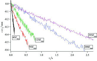
Figure 1: (Color online) Position of the center-of-mass of the atomic cloud derived from time-of-flight detection data, as a function of holding time $\tau$ in the optical lattice for the potential depths 45$E_{\mathrm{rec}}$ (black), 95$E_{\mathrm{rec}}$ (red), 125$E_{\mathrm{rec}}$ (green), 200$E_{\mathrm{rec}}$ (blue) and 395$E_{\mathrm{rec}}$ (purple), for a detuning of $-40\Gamma$.

The arrival time of an atom to the time-of-flight probe is a function of its initial position and initial velocity. From the average arrival time, the average position, $\langle x\rangle=\langle\dot{x}\rangle\tau$, follows directly. The linear evolution of the drift, evidencing the ‘stop-and-go’ dynamics, is observed from the data presented in Fig. 1, where a faster drift due to the gravitational tilt is also observed for shallower potentials.

IV.2.1 Mobility

In order to extract the velocity of the drift $\langle\dot{x}\rangle$, straight lines are fitted to curves like the ones in Fig. 1. Figure 2a shows results for a range of data, with $\langle\dot{x}\rangle$ as function of the potential depth for the detunings $-30\Gamma$ and $-40\Gamma$.

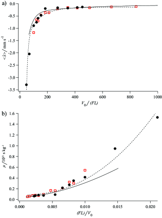
Figure 2: (Color online) (a) Derived drift velocity, $\langle\dot{x}\rangle$, as a function of potential depth, $V_{0}$, for the detunings $-30\Gamma$ (open squares), and $-40\Gamma$ (circles). (b) the same data, but plotted as the mobility, $\mu$ as a function of $(FL)/V_{0}$. The solid line is from a semi-classical Monte-Carlo simulation, while the dashed line is from a simplified classical simulation.

In Fig. 2b we display the same data, but now scaled as the mobility $\mu$ as a function of the constant force $F$ divided by the potential depth. This allows for a more direct comparison with the general theoretical treatment in Risken:1989 . Such a comparison must be made with care, since in Risken:1989 a spatially uniform friction is assumed, whereas our experimental conditions are such that the damping force that acts on individual atoms depends strongly on position and kinetic energy. Moreover, even with a simplified model for a friction force, the coefficient of friction will vary with detuning Dalibard:1989p1149 . Nevertheless, fluctuation-induced drift in the tilted potential is clearly demonstrated.

IV.2.2 Running and locked states

By analyzing the velocity distributions obtained by time-of-flight detection, the fraction of atoms in the running state compared with the total amount of atoms, $N_{\mathrm{run}}/N_{\mathrm{tot}}$ , can be extracted Jersblad:2004p1224 ; Dion:2005p1121 ; Hagman:2008p1134 . Assuming that the momentum distribution corresponds to a (truncated) Gaussian core of trapped atoms, with wide wings corresponding to untrapped atoms, we can calculate approximate numbers for $N_{\mathrm{run}}/N_{\mathrm{tot}}$ and by Gaussian fits to the momentum distributions. The results of this for the same data used to observe the drift is shown in Fig. 3a.

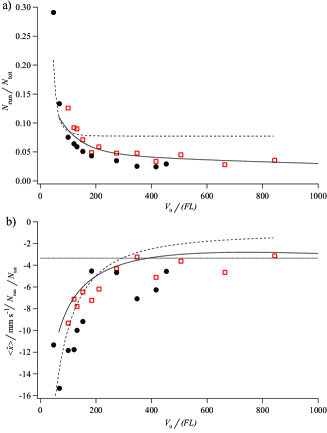
Figure 3: (Color online) (a) The fraction of unlocked atoms, as a function of potential depth, $V_{0}$, for the detunings, $-30\Gamma$ (open squares), and $-40\Gamma$ (circles) The solid line represents the semi-classical Monte-Carlo simulation, and the dashed line is the classical simulation. (b) The drift divided by the fraction of atoms is the running state versus the potential depths. A straight line indicates the recoil velocity. Note that velocity is defined to be positive upwards

Within our range of detunings and irradiances, the fraction of the atoms that are free is typically just a few percent. For potential depths smaller then about 200$E_{\mathrm{rec}}$, the fraction of atoms in the running state increases drastically, and for the shallowest potentials we use, it gets as high as about 25%. This behaviour has striking similarities with Fig. 2a, where the average velocity downwards due to gravity also increases drastically for the same potential depths. As an attempt to investigate the dependence between the drift and the fraction of atoms in the ‘running state’ further, in Fig. 3b we plot $\langle\dot{x}\rangle/(N_{\mathrm{run}}/N_{\mathrm{tot}})$ versus the potential depth. From this it is clear that the drift, not being constant, depends not only on the fraction of untrapped atoms but also on something else.

V Simulations

V.1 Semi-Classical Monte-Carlo Method

With a semi-classical Monte-Carlo simulation of the atom-laser interaction Jonsell:2006p1132 ; Svensson:2008p1137 , we derive theoretical data corresponding to all experimental curves shown. In these simulations, the laser field and the motion of the atoms are treated classically, which enables tracking of the position and momentum of each particle, while the internal state of the atom is treated quantum mechanically, using the true degenerate level structure of the $F_{\mathrm{g}}=4\rightarrow F_{\mathrm{e}}=5$ transition. In addition, the presence of the excited $F_{\mathrm{e}}=4$ level is also included Svensson:2008p1137 . Diffusion and friction arise “naturally” from the laser-atom interaction and are position and velocity dependent, as in the experiment.

The simulations comprise 15000 non-interacting atoms, starting from an initial cloud contained in a single lattice well, at a temperature of $5\ \mu\mathrm{K}$. The drift velocity is obtained by calculating the median position of the atoms at the end of the simulation and dividing by the duration of the simulation ($\sim 50\ \mathrm{ms}$). This is necessary because a direct calculation of $\left\langle\dot{x}\right\rangle$ is affected by the presence of a few high-velocity atoms, corresponding atoms that become untrapped and never get recaptured by the lattice. Such atoms are believed to be also present in the experiment, but drift out of the lattice and never get detected.

The optical lattice is here one dimensional (along the vertical), which means that an exact quantitative agreement cannot be expected, but all qualitative features in the experiment are reproduced, and so are the orders of magnitude of the mobility, the fractional populations, and the potential depths where significant features occur. Also, the fraction of atoms in the running state is calculated much more precisely from total energies and positions of the individual atoms, than it can be determined from the experimental time-of-flight data. The results, smoothed out to remove the fluctuations due to the small sample size, are shown together with the experimental data in Figs. 2 and 3.

One of the constraints of the current experimental setup is the use of gravity as the external force. This means that the variation of $FL/V_{0}$ can only be achieved by a change in $V_{0}$. However, $V_{0}$ is not independently controllable, but it depends on the irradiance of the lasers and their detuning with respect to the atomic transition. These in turn affect friction (Sisyphus cooling) and diffusion (photon scattering), and therefore also the temperature of the atoms, such that it can be seen as being a function of the optical lattice potential depth (see, e.g., Castin:1991 ; Grynberg:2001p1099 ).

To investigate how this affects the mobility, we have run simulations at constant potential depth for different values of the external force. In Fig. 4(a), the simulation result previously shown in Fig. 2(b) is plotted along with the mobility obtained varying $F$, for two different values of $V_{0}$.

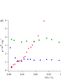
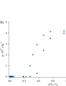
Figure 4: (Color online) Mobility calculated from semi-classical Monte-Carlo simulations. $+$: constant force $F=mg$ and varying $V_{0}$ [same data as full line in Fig. 2(b)]; $\circ$: varying $F$ and constant $V_{0}=70E_{\mathrm{rec}}$; $\times$: varying $F$ and constant $V_{0}=140E_{\mathrm{rec}}$. The detuning is $-30\Gamma$. Panels (a) and (b) differ only by the scaling of the abscissa.

Over the range covered by the experiment, the mobility now appears constant, with a value dependent on the potential depth. Further increasing the value of the external force, Fig. 4(b), the well-known behavior of Brownian particles in tilted potentials emerges, with a transition region between locked and running states Risken:1989 . It thus appears that the variation of the mobility as a function of $V_{0}$, Fig. 2, reflects the fact that it is the laser irradiance, and not strictly the potential depth, that is modified. In addition, the current experiment probes a region corresponding to a low-mobility locked state, in accord with the fact that most atoms have an energy below the well-to-well barrier height Jersblad:2004p1224 ; Dion:2005p1121 . Note that the semi-classical model used here cannot reproduce the Doppler cooling Dalibard:1989p1149 ; cool:nobel98 that will become important as the velocity of the atoms increases.

V.2 Classical Approach

In order to check the generality of the system and relevance of an analysis in terms of a Fokker-Planck equation, as in Eq. (1), we also perform a simple, completely classical Monte-Carlo simulation for the Langevin equation corresponding to Eq. (1), for a 1D system with classical particles in a tilted washboard potential, as in Eq. (2). In this simulation, we let the noise term and the friction scale linearly with the potential depths. For simplicity and generalization we take a uniform friction. The results are presented together with the experimental data in Figs. 2 and 3. The basic characteristics of our system are reproduced.

VI Conclusion

To conclude, we have made a quantitative study of how random isotropic fluctuations, together with a very small bias force, gives rise to an average drift. When the fraction between bias force and trapping potential, $F/V_{0}$ is varied, the magnitude of this drift can change. The system can be well described by a Fokker-Planck equation formalism, and the experimental control, together with the precision in the measurements, make the system suitable as a general testbed for studies of fundamental fluctuation phenomena. To emphasize this, we qualitatively reproduce our data with a simplified classical simulation, as well as with a careful semi-classical Monte-Carlo simulation of the laser cooling setup. Our results also evidence the ‘stop-and-go’ nature of the dynamics of the atoms, where they continuously exchange between being trapped in potential wells and travelling over many wells Marksteiner:1996p1152 ; Ellmann:2001p1222 ; Dion:2005p1121 ; Jonsell:2006p1132 .

One of the constraints of the present experiment is the use of gravity as the bias force. This leaves the potential depth $V_{0}$ as the main variable parameter, but it is only accessible through the laser irradiance, which also modifies diffusion and friction. One possible solution would be the introduction of an additional laser beam, using its radiation pressure as the bias force. Moreover, it is possible to operate the optical lattice far-detuned from the atomic resonance, where it only serves as a (conservative) potential. Extra laser fields could provide diffusion and friction, allowing the exploration of a broad range of scenarios.

- (1) H. Risken, The Fokker-Planck Equation, 2nd ed. (Springer, Berlin, 1989).
- (2) M. Borromeo and F. Marchesoni, Phys. Rev. Lett. 84, 203 (2000).
- (3) M. Borromeo and F. Marchesoni, Chaos 15, 026110 (2005).
- (4) C. Jarzynski, Phys. Rev. Lett. 78, 2690 (1997).
- (5) D. J. Evans, E. G. D. Cohen, and G. P. Morriss, Phys. Rev. Lett. 71, 2401 (1993).
- (6) D. J. Evans and D. J. Searles, Phys. Rev. E 50, 1645 (1994).
- (7) G. E. Crooks, Phys. Rev. E 60, 2721 (1999).
- (8) U. Seifert, Phys. Rev. Lett. 95, 040602 (2005).
- (9) G. M. Wang, E. M. Sevick, E. Mittag, D. J. Searles, and D. J. Evans, Phys. Rev. Lett. 89, 050601 (2002).
- (10) J. Liphardt, S. Dumont, S. B. Smith, I. Tinoco Jr., and C. Bustamante, Science 296, 1832 (2002).
- (11) P. Reimann, Phys. Rep. 361, 57 (2002).
- (12) P. Hänggi and F. Marchesoni, Rev. Mod. Phys. 81, 387 (2009).
- (13) F. Renzoni, Adv. At. Mol. Opt. Phys. 57, 1 (2009).
- (14) G. Grynberg and C. Robilliard, Phys. Rep. 355, 335 (2001).
- (15) P. S. Jessen and I. H. Deutsch, Adv. At. Mol. Opt. Phys. 37, 95 (1996).
- (16) Note that we had previously mentionned in Sjolund:2007p1141 that the effect of gravity was three orders of magnitude smaller than the recoil energy, which is erroneous.
- (17) P. Sjölund, S. J. H. Petra, C. M. Dion, S. Jonsell, M. Nylén, L. Sanchez-Palencia, and A. Kastberg, Phys. Rev. Lett. 96, 190602 (2006).
- (18) P. Sjölund, S. J. H. Petra, C. M. Dion, H. Hagman, S. Jonsell, and A. Kastberg, Eur. Phys. J. D 44, 381 (2007).
- (19) H. Hagman, C. M. Dion, P. Sjölund, S. J. H. Petra, and A. Kastberg, Europhys. Lett. 81, 33001 (2008).
- (20) J. Dalibard and C. Cohen-Tannoudji, J. Opt. Soc. Am. B 6, 2023 (1989).
- (21) S. Chu, Rev. Mod. Phys. 70, 685 (1998); C. Cohen-Tannoudji, ibid. 70, 707 (1998); W. D. Phillips, ibid. 70, 721 (1998).
- (22) Y. Castin, J. Dalibard, and C. Cohen-Tannoudji, in Light Induced Kinetic Effects on Atoms, Ions, and Molecules, edited by L. Moi, S. Gozzini, C. Gabbanini, E. Arimondo, and F. Strumia (ETS Editrice, Pisa, 1991), pp. 5–24.
- (23) M. Gatzke, G. Birkl, P. S. Jessen, A. Kastberg, S. L. Rolston, and W. D. Phillips, Phys. Rev. A 55, R3987 (1997).
- (24) S. Marksteiner, K. Ellinger, and P. Zoller, Phys. Rev. A 53, 3409 (1996).
- (25) G. Raithel, G. Birkl, A. Kastberg, W. D. Phillips, and S. L. Rolston, Phys. Rev. Lett. 78, 630 (1997).
- (26) W. Greenwood, P. Pax, and P. Meystre, Phys. Rev. A 56, 2109 (1997).
- (27) C. M. Dion, P. Sjölund, S. J. H. Petra, S. Jonsell, and A. Kastberg, Europhys. Lett. 72, 369 (2005).
- (28) H. Ellmann, J. Jersblad, and A. Kastberg, Eur .Phys. J. D 13, 379 (2001).
- (29) L. Sanchez-Palencia, P. Horak, and G. Grynberg, Eur. Phys. J. D 18, 353 (2002).
- (30) S. Jonsell, C. M. Dion, M. Nylen, S. J. H. Petra, P. Sjölund, and A. Kastberg, Eur. Phys. J. D 39, 67 (2006).
- (31) J. Jersblad, H. Ellmann, K. Støchkel, A. Kastberg, L. Sanchez-Palencia, and R. Kaiser, Phys. Rev. A 69, 013410 (2004).
- (32) H. Ellmann, J. Jersblad, and A. Kastberg, Eur. Phys. J. D 22, 355 (2003).
- (33) G. Grynberg, B. Lounis, P. Verkerk, J.-Y. Courtois, and C. Salomon, Phys. Rev. Lett. 70, 2249 (1993).
- (34) D. A. Steck, “Cesium D Line Data,” available online at http://steck.us/alkalidata (revision 2.1, 1 September 2008).
- (35) F. Svensson, S. Jonsell, and C. M. Dion, Eur. Phys. J. D 48, 235 (2008).