Quantum state engineering with flux-biased Josephson phase qubits by rapid adiabatic passages

Abstract

In this paper, the scheme of quantum computing based on Stark-chirped rapid adiabatic passage (SCRAP) technique [Phys. Rev. Lett. 100, 113601 (2008)] is extensively applied to implement the quantum-state manipulations in the flux-biased Josephson phase qubits. The broken-parity symmetries of bound states in flux-biased Josephson junctions are utilized to conveniently generate the desirable Stark-shifts. Then, assisted by various transition pulses, universal quantum logic gates as well as arbitrary quantum-state preparations could be implemented. Compared with the usual $\pi$-pulses operations widely used in the experiments, the adiabatic population passages proposed here are insensitive to the details of the applied pulses and thus the desirable population transfers could be satisfyingly implemented. The experimental feasibility of the proposal is also discussed.

PACS number(s): 85.25.Cp, 03.67.Lx, 42.50.Dv.

I Introduction

Quantum state engineering (QSE) based on superconducting Josephson circuits (SJCs) makhlin has been stimulated by the encouraging prospects of quantum computing (QC) and quantum information processing (QIP) you ; clarke ; wendin ; devoret . The SJCs include the charge- nakamura , flux- friedman ; mooij , and phase qubits Martinis ; Simmonds ; berkley as well as their variants vion ; koch ; manucharyan . Moreover, QSE with SJCs is also a crucial approach to investigate the fundamental quantum phenomena, such as geometric phase leek and non-locality Wei3 ; ansmann . Note that most of the current experiments for QSE employ the technique that is sensitive to the exact design of the applied pulses. A typical example is that the so-called $\pi$-pulse is usually exactly designed to transfer the population from one quantum state to another. However, these duration-sensitive operations might not be practically the most optimal approaches to implement the desirable quantum manipulations with sufficiently-high fidelity and efficiency.

Besides the exactly-designed pulse operations, adiabatic passage (AP) technique developed in atomic physics is also an efficient strategy for quantum-state control. This technique possesses certain significant advantages, such as high transfer efficiency, robustness to environment noises, and less limits on the designs of the operational pulses. It is well-known that the main APs include such as the stimulated Raman AP (STIRAP) bergmann , Stark chirped rapid AP (SCRAP) yatsenko1 ; rangelov ; oberst , and piecewise AP (PAP) shapiro , etc.. Certainly, all of these methods are competent for various population transfers. But, certain limits still exist in these APs. For example, STIRAPs are not immune to the induced ac Stark shifts rickes . Also, PAP demonstrated in recent experiments still needs a series of ultrafast pulses to simultaneously control the switches of two pulses and phase holdings. This further requires the superb operating techniques. In contrast, SCRAP realized in the recent experiment oberst only needs relevant controls on the amplitudes of pulses and thus could be immune to the inhomogeneous level broadening.

AP technique has also been used in SJCs for various applications, (see, e.g., kis ; siewert ; xia ; song ; wei2008 ). For example, the STIRAP technique was utilized to prepare Fock state siewert of a nanomechanical oscillator coupled to a Cooper-pair box, two-qubit and three-qubit entangled states in coupled Josephson flux circuits were proposed xia ; song , etc.. In particular, in Ref. wei2008 we proposed an effective approach, by using the SCRAP technique, to implement the fundamental logic gates without precisely designing the durations of the operations. In this paper, we further generalize such an idea to implement the QSE with flux-biased Josephson circuits, including the single-qubit phase shift and also the $\sigma_{x}$-rotation operation, as well as the two-qubit iSWAP gate. Our basic idea is to introduce a controllable flux-perturbation to chirp the transition frequency of a selected flux-biased qubit. Then, by properly controlling the amplitude ratio of perturbation to the transition driving, desirable population transfers between the selected quantum states could be achieved with sufficiently-high efficiency. Based on these operations, various single- and two-qubit logic gates in these SJCs could be implemented without exactly designing the durations of the applied adiabatic pulses. Furthermore, arbitrary superposition of the logic states could also been implemented, in principle. Given the flux-biased Josephson phase qubits and their manipulations have already been demonstrated, the present proposal should be experimentally feasible.

The paper is organized as follows: In Sec. II we give a brief review of the usual $\pi$-pulse coherent excitation, and the SCRAP technique used in atomic physics is also included. Subsequently, we give a simple description of the flux-biased phase qubit, a detailed approach for population adiabatic transfers, as well as controllable construction of superposition state. In Sec. III, we discuss how to implement the two-qubit gate with capacitively-coupled flux-biased phase qubits by the proposed SCRAP technique. Finally, conclusions and discussions are given in Sec. IV.

II Population transfers between driven two levels

Two-level system is a fundamental model in quantum physics. In QIP the basic information element (i.e., qubit) is encoded by a well-defined two-level system. There are many approaches to implement the population transfers between the two levels of the qubit. Roughly, these approaches can be classified into the nonadiabatic- and adiabatic passages bergmann .

II.1 Nonadiabatic population passages: $\pi$-pulse coherent excitations

The Hamiltonian of a single qubit driven by an external field can be generally written as ($\hbar\equiv 1$)

$$H_{s}(t)=\frac{\omega_{0}}{2}\sigma_{z}+R(t)\sigma_{x},$$ (1)

where $\sigma_{z}$ and $\sigma_{x}$ refer to the Pauli spin operators and $\omega_{0}$ the transition frequency of the qubit. $R(t)=\Omega(t)\cos(\upsilon t)$ is the driving term with $\upsilon$ being the pulse frequency and $\Omega(t)=\varepsilon(t)\mu/\hbar$ the Rabi frequency. Here, $\varepsilon(t)$ is the amplitude of the applied pump pulse, and $\mu$ the matrix element of electric dipole moment. Suppose that the applied pump $I_{ac}(t)=\varepsilon(t)\cos(\upsilon t)$ is resonant with the qubit, i.e., $\upsilon=\omega_{0}$. In the interaction picture, Eq. (1) reduces to

$$H_{int}(t) = \exp{(it\omega_{0}\sigma_{z}/2)}R(t)\sigma_{x}\exp{(-it\omega_{0}\sigma_{z}/2)}$$ (2)

$$= \frac{\Omega(t)}{2}\sigma_{x},$$

under the usual rotating-wave approximation (RWA). Correspondingly, the solution to the Schrödinger equation

$$i\frac{\partial U_{int}(t)}{\partial t}=H_{int}(t)U_{int}(t),$$ (3)

can be expressed as

$$U_{int}(t) = \exp{\left(-i\int_{0}^{t}H_{int}(t^{\prime})dt^{\prime}\right)}$$ (4)

$$= \cos\frac{A(t)}{2}\textbf{I}-i\sin\frac{A(t)}{2}\sigma_{x}.$$

Here, $A(t)=\int_{0}^{t}\Omega(t^{\prime})dt^{\prime}$ and I is an unit matrix. This implies that, if the qubit is initially prepared in the ground state, then at the time $t$ the probability for the qubit evolving to the excited state is $P_{e}(t)=(1-\cos A(t))/2$. Therefore, in order to realize complete population inversion, the pulse area must be precisely designed as $\pi$. Any deviation from the precise pulse area may result in dynamical error for the desirable population inversion.

II.2 Adiabatic population passages: Stark Chirps

For loosening the above rigorous requirement on exactly designing pulse area and improving the operational reliability, we add a controllable perturbation to the Hamiltonian (1), i.e.,

$$H^{\prime}_{s}(t)=\frac{\omega_{0}}{2}\sigma_{z}+R(t)\sigma_{x}-\frac{\Delta(t)}{2}\sigma_{z}.$$ (5)

In the interaction picture, the above Hamiltonian reduces to

$$H^{\prime}_{int}(t)=\frac{1}{2}\left(\begin{array}[]{cc}0&\Omega(t)\\ \Omega(t)&2\Delta(t)\end{array}\right).$$ (6)

Note that this Hamiltonian is as the same as that in the original SCRAP scheme yatsenko1 , wherein the Hamiltonian is derived in the Schrödinger picture. Also, the pump pulse $I_{ac}(t)$ applied in the present scheme is required to be resonant with the qubit. Certainly, compared with the transition frequency $\omega_{0}$ of the qubit, the controllable Stark-shift term $\Delta(t)$ should be sufficiently small. For convenience, we rewrite the Hamiltonian (6) as

$$H^{\prime\prime}_{int}(t) = \frac{\epsilon(t)}{2}\left(\begin{array}[]{cc}0&\frac{\Omega(t)}{\sqrt{\Delta^{2}(t)+\Omega^{2}(t)}}\\ \frac{\Omega(t)}{\sqrt{\Delta^{2}(t)+\Omega^{2}(t)}}&\frac{2\Delta(t)}{\sqrt{\Delta^{2}(t)+\Omega^{2}(t)}}\end{array}\right)$$ (9)

$$= \frac{\epsilon(t)}{2}\left(\begin{array}[]{cc}0&\sin 2\vartheta(t)\\ \sin 2\vartheta(t)&2\cos 2\vartheta(t)\\ \end{array}\right),$$ (12)

where $\epsilon(t)=\sqrt{\Delta^{2}(t)+\Omega^{2}(t)}$, and $\tan 2\vartheta(t)=\Omega(t)/\Delta(t)$. The instantaneous eigenvalues of the above time-dependent Hamiltonian can be straightforwardly written as: $\mu_{\pm}(t)=(\Delta(t)\pm\sqrt{\Delta^{2}(t)+\Omega^{2}(t)})/2$ with the corresponding eigenvectors,

$$|\lambda_{+}(t)\rangle=\sin\vartheta(t)\,|0\rangle+\cos\vartheta(t)\,|1\rangle,$$ (13a)

$$|\lambda_{-}(t)\rangle=\cos\vartheta(t)\,|0\rangle-\sin\vartheta(t)\,|1\rangle.$$ (13b)

In the new Hilbert space spanned by the vectors $|\lambda_{-}(t)\rangle$ and $|\lambda_{+}(t)\rangle$, the Hamiltonian (6) reads (see Appendix)

$$H_{new}(t)=\left(\begin{array}[]{cc}\mu_{-}(t)&-i\dot{\vartheta}(t)\\ i\dot{\vartheta}(t)&\mu_{+}(t)\\ \end{array}\right).$$ (14)

Under the adiabatic approximation,

$$\frac{1}{2}\left|\Omega(t)\frac{d\Delta(t)}{dt}-\Delta(t)\frac{d\Omega(t)}{dt}\right|\ll\left(\Delta^{2}(t)+\Omega^{2}(t)\right)^{3/2},$$ (15)

Hamiltonian Eq. (14) can be further simplified to

$$H_{ad}(t)=\left(\begin{array}[]{cc}\mu_{-}(t)&0\\ 0&\mu_{+}(t)\\ \end{array}\right).$$ (16)

The vanished nondiagonal elements denote that there is not any transition between the two instantaneous eigenstates $|\lambda_{-}(t)\rangle$ and $|\lambda_{+}(t)\rangle$. This implies that the qubit would passage individually along one of the two adiabatic paths, as long as $\vartheta(t)$ changes slowly. As a consequence, the generic solution of the system takes the form

$$|\Psi(t)\rangle =v_{-}(0)\exp(-i\int_{0}^{t}\mu_{-}(t^{\prime})dt^{\prime})|\lambda_{-}(t)\rangle+$$ (17)

$$\,\,\,v_{+}(0)\exp(-i\int_{0}^{t}\mu_{+}(t^{\prime})dt^{\prime})|\lambda_{+}(t)\rangle.$$

Obviously, although the population of an adiabatic state is conservational for no coupling between adiabatic states, the components in the states $|0\rangle$ and $|1\rangle$ can still vary with the time-dependent $\vartheta(t)$. In principle, one can realize arbitrary population distributions in $|0\rangle$ and $|1\rangle$ along one selected adiabatic path. As an obvious advantage, the population transfer presented here is not sensitive to the pulse area.

When the pump pulse is absent, the Hamiltonian Eq. (6) becomes $H_{z}=\Delta(t)|1\rangle\langle 1|$. This indicates that a Stark-chirping pulse is sufficient to produce a phase shift gate $U_{z}(\alpha)=\exp(i\alpha|1\rangle\langle 1|)$ with $\alpha=-\int_{t_{0}}^{t_{f}}\Delta(t^{\prime})dt^{\prime}$:

$$|0\rangle\longrightarrow|0\rangle,\,\,|1\rangle\longrightarrow e^{i\alpha}|1\rangle.$$ (18)

This is similar to the idea by lowering the potential to implement the fast qubit’s readout cooper . This is because that the Stark pulse does not destruct the population distributions in the states $|0\rangle$ and $|1\rangle$, but just leads to the phase accumulations bialczak . By combining the Rabi pulse for transferring the populations between the two levels and the Stark pulse for phase shift operation, one can implement arbitrary superposition of the states $|0\rangle$ and $|1\rangle$, with controllable probabilities and relative phase.

(i) Implement the $\sigma_{x}$-rotation operation. We design a pulse sequence shown in Fig. 2(a): apply only the Stark pulse at the first for satisfying the initial condition $\vartheta(t_{0})=0$; and then a pump pulse is applied but it switches off prior to Stark pulse for satisfying the condition $\vartheta(t_{f})=\pi/2$. This pulse sequence yields the following population inversion

$$\!\!\!\!\!\!\!\!\!\!\!\!\!\!\!\!\!\!\!\!\!\!H_{inv}:\left\{\begin{split}|\Psi(t_{0})\rangle=|0\rangle\xrightarrow{|\lambda_{-}(t)\rangle}|\Psi(t_{f})\rangle=-|1\rangle\\ |\Psi(t_{0})\rangle=|1\rangle\xrightarrow{|\lambda_{+}(t)\rangle}|\Psi(t_{f})\rangle=\;\;\;|0\rangle\end{split}\right.$$ (19)

along the adiabatic paths $|\lambda_{+}(t)\rangle$ and $|\lambda_{-}(t)\rangle$, respectively. If the qubit resides in $|0\rangle$ (or $|1\rangle$) originally, it would evolve to the state $|1\rangle$ (or $|0\rangle$) along the adiabatic path $|\lambda_{-}(t)\rangle$ (or $|\lambda_{+}(t)\rangle$). After eliminating the additional phase via a phase-shift gate operation $H_{z}(\pi)$ described above, one can realize single-qubit NOT gate, i.e., $U_{NOT}=H_{z}(\pi)H_{inv}$. Certainly, this implemented process needs to be adiabatic, otherwise the state will evolve along one of the two Landau-Zener tunneling paths, which suppresses the desirable complete population inversion between the two logic states.

(ii) Implement the Hadamard gate. As another example, we set the pulses sequence as (see Fig. 2(b)): Stark pulse precedes pump pulse to obtain the initial condition $\vartheta(t_{0})=0$ and switches off prior to the pump pulse resulting in $\vartheta(t_{f})=\pi/4$. This means that

$$\!\!\!\!\!\!\!\!\!\!\!\!\!\!\!\!\!\!\!\!\!\!R_{h}:\left\{\begin{split}|\Psi(t_{0})\rangle=|0\rangle\xrightarrow{|\lambda_{-}(t)\rangle}|\Psi(t_{f})\rangle=\frac{|0\rangle-|1\rangle}{\sqrt{2}}\\ |\Psi(t_{0})\rangle=|1\rangle\xrightarrow{|\lambda_{+}(t)\rangle}|\Psi(t_{f})\rangle=\frac{|0\rangle+|1\rangle}{\sqrt{2}}\end{split}\right.$$ (20)

This is the standard Hadamard gate operation.

II.3 Physical implementation with single flux-biased phase qubit

SJCs provide a favorable approach to implement QC due to its nonlinearity. Especially, flux-biased phase qubits are typically utilized to perform QC with superconducting circuits Martinis ; Simmonds .

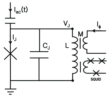
Figure 1: Circuit schematic for a single flux-biased phase qubit Martinis , where the $X$ symbol denotes the JJ. $I_{ac}(t)$ is the microwave pump pulse and $I_{\phi}$ is the biased dc-current.

Typically, a flux-biased phase qubit is generated by a superconducting loop (of inductance $L$) biased by a magnetic flux $\Phi_{e}$ and interrupted by a Josephson junction (JJ) (with capacitance $C$ and critical current $I_{0}$). The advantage of this structure is that the generated qubit can be isolated well from the strongly-dissipative bias leads martinis3 . Using Kirchhoff’s law, the currents along all the branches of the circuit shown in Fig. 1 satisfy the equation

$$I_{J}+I_{C}+I_{L}=I_{ac}(t).$$ (21)

Using the Josephson current-phase relation $I_{J}=I_{0}\sin\delta$ and the voltage-phase relation $\dot{\delta}=2\pi V_{J}/\Phi_{0}$, the above equation can be straightforward rewritten as ansmann2

$$I_{0}\sin\delta(t)+C_{J}\frac{d}{dt}\frac{\Phi_{0}}{2\pi}\dot{\delta}+\int\frac{V_{J}}{L}dt=I_{ac}(t).$$ (22)

This equation can be further expressed by Clarke

$$C_{J}(\frac{\Phi_{0}}{2\pi})^{2}\ddot{\delta}+\frac{\partial U(\delta)}{\partial{\delta}}=0,$$ (23)

with

$$U(\delta) = -\frac{\Phi_{0}}{2\pi}I_{0}\cos\delta-\frac{\Phi_{0}}{2\pi}I_{ac}(t)\delta$$ (24)

$$+\int\frac{\Phi_{0}}{2\pi L}\left(\frac{\Phi_{0}}{2\pi}\delta-\Phi_{ex}\right)d\delta$$

$$= E_{J}\left(\frac{(\delta-\phi_{b})^{2}}{2\lambda}-\cos\delta\right)-\frac{\Phi_{0}}{2\pi}I_{ac}(t)\delta.$$

Here, $\delta$ is gauge invariant phase difference (macroscopic variable) of the JJ, $\Phi_{ex}=MI_{\phi}$ is the applied magnetic flux, $E_{J}=I_{0}\Phi_{0}/2\pi$ the JJ coupling energy, and $\lambda=2\pi I_{0}L/\Phi_{0}$, $\phi_{b}=2\pi\Phi_{ex}/\Phi_{0}$. Also, $I_{\phi}=I_{\phi 0}+I_{dc}(t)$ is the biased current with $I_{\phi 0}$ being the constant part and $I_{dc}(t)$ the level-chirping part used for generating the Stark shift.

The above potential function $U(\delta)$ can be divided into two parts: time-independent and time-dependent ones, i.e.,

$$U(\delta)=U_{0}(\delta)+V(t),$$ (25)

with

$$U_{0}(\delta)=E_{J}\left(\frac{(\delta-\phi_{b0})^{2}}{2\lambda}-\cos\delta\right),$$

$$V(t)=-\frac{\Phi_{0}M}{2\pi L}I_{dc}(t)\delta-\frac{\Phi_{0}}{2\pi}I_{ac}(t)\delta,$$

where $\phi_{b0}=2\pi I_{\phi 0}M/\Phi_{0}$.

Obviously, Eq. (23), i.e., the equation for the gauge invariant phase difference $\delta$, can be interpreted as that for the motion of a particle with mass $m=C_{J}(\Phi_{0}/(2\pi))^{2}$ moving in the potential $U(\delta)$. Certainly, the shape of this potential can be controlled by adjusting the biased current $I_{\phi}$, which indirectly changes magnetic flux though the loop. The bounded particle moving in the potential would have discrete energy levels. It is well known that all bound states of natural atoms/molecules have definite parities, and therefore the so-called electric-dipole selection rule determines all the possible transitions between the selected levels. This rule forbids the transition between the states with the same parity. However, in certain artificial atoms generated by, e.g., the present SJCs, the bound states lose the definite parities, and thus the electric-dipole transitions between arbitrary two levels are possible. This provides a convenient way to design the requirable pulses for implementing the above population transfers.

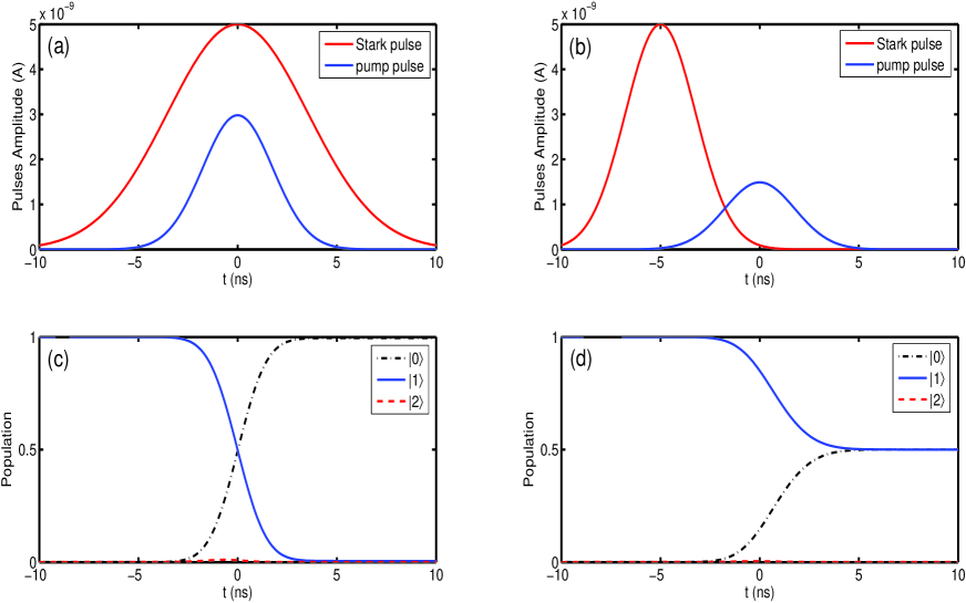
Figure 2: (Color online) Population evolutions in a single flux-biased phase qubit based on the proposed SCRAP. (left) Population inversion operation achieved by using the adiabatic pulses (a) with the parameters $\mathrm{I_{dc}(t)=5exp(-t^{2}/5^{2})}$ nA, $\mathrm{\Omega(t)=2.98exp(-t^{2}/2.5^{2})}$ nA. Here, the qubit initially resides in the state $|1\rangle$, after the designed SCRAP, $|0\rangle$ is fully populated. The population in the upper level (i.e., $|2\rangle$) is significantly small (its largest value is typically less than $1\%$), and thus during the SCRAP the influence of this level is negligible. (right) Preparation of the superposition state $(|0\rangle+|1\rangle)/\sqrt{2}$ from the state $|1\rangle$ by the SCRAP with the adiabatic pulses $\mathrm{I_{dc}(t)=5exp(-(t+5)^{2}/2.5^{2})}$ nA, $\mathrm{\Omega(t)=1.495exp(-t^{2}/2.5^{2})}$ nA.

First, a proper magnetic flux is applied to let the junction has several bound levels in the potential. Usually, the lowest two levels with splitting-frequency $\omega_{10}=(E_{1}-E_{0})/\hbar$ are selected to encode a JJ phase qubit, and the third one $|2\rangle$ might be involved during the qubit operations.

Second, in order to perform the expected SCRAP introduced above, a microwave pump pulse $I_{ac}(t)=\varepsilon(t)\cos\,\omega_{10}t$ and a controllable Stark pulse $I_{dc}(t)$ are applied to couple the qubit states, and chirp the qubit’s transition frequency, respectively. Under these drivings, the Hamiltonian of the above flux-biased JJ reads steffen2

$$\bar{H}_{s}(t) =\bar{H}_{0}+V(t),\$$ (26)

with

$$\bar{H}_{0} =p^{2}/2m+U_{0}(\delta)=\sum_{i=0,1,2}E_{i}|i\rangle\langle i|,$$

and

$$V(t) =-(\Phi_{0}/2\pi)\Big{[}\frac{M}{L}I_{dc}(t)+I_{ac}(t)\Big{]}\delta$$

$$=-(\Phi_{0}/2\pi)\Big{[}\frac{M}{L}I_{dc}(t)+I_{ac}(t)\Big{]}\sum_{i,j=0,1,2}|i\rangle\langle j|\delta_{ij},$$

where $\delta_{ij}=\langle i|\delta|j\rangle$. We assume that Stark shifts induced by the pump pulse are ignorable compared to those induced by the Stark pulse, and also that couplings (between the selected levels) induced by the Stark pulse are negligible compared to those induced by the pump pulse. In the interaction picture and under the usual rotating-wave appropriation, the above Hamiltonian can be rewritten as

$$\tilde{H}_{int}(t) =\exp(it\bar{H}_{0})V(t)\exp(-it\bar{H}_{0})$$

$$=-\frac{\Phi_{0}}{2\pi}\left(\begin{array}[]{ccc}0&\kappa\delta_{01}&0\\ \kappa\delta_{10}&\tilde{\Delta}_{1}(t)&\kappa\delta_{12}\exp(i\nu t)\\ 0&\kappa\delta_{21}\exp(-i\nu t)&\tilde{\Delta}_{2}(t)\\ \end{array}\right),$$ (30)

where $\kappa=\Omega(t)/2,\nu=\omega_{10}-\omega_{21},\tilde{\Delta}_{1}(t)=MI_{dc}(t)(\delta_{11}-\delta_{00})/L,\tilde{\Delta}_{2}(t)=MI_{dc}(t)(\delta_{22}-\delta_{00})/L$. For clarity, we return to the Schrödinger picture, and the above equation can be rewritten as

$$\bar{H}(t) =-\frac{\Phi_{0}}{2\pi}\left(\begin{array}[]{ccc}0&\kappa\delta_{01}&0\\ \kappa\delta_{10}&\tilde{\Delta}_{1}(t)&\kappa\delta_{12}\\ 0&\kappa\delta_{21}&\tilde{\Delta}_{2}(t)+h\nu/\Phi_{0}\\ \end{array}\right).$$ (35)

With the experimental parameters Simmonds ; johnson2 $I_{0}=8.351$ $\mu$A, $C_{J}=1.2$ pF, $L=168$ pH, $L/M=81$, and $I_{\phi 0}=923.7$ $\mu$A, one can numerically confirm that four bound states (levels) exist in the left well of the potential $U(\delta)$, and also $\delta_{00}=1.571$, $\delta_{11}=1.598$, $\delta_{22}=1.633$, $\delta_{01}=\delta_{10}=0.076$, $\delta_{12}=\delta_{21}=0.109$, $\delta_{02}=\delta_{20}=-0.006$, $\omega_{10}/2\pi=10.981$ GHz, $\omega_{21}/2\pi=10.340$ GHz.

Fig. 2 shows the desirable single qubit operation. (c) denotes that, under the pulse sequence in (a), the population in the state $|1\rangle$ can be completely inverted to the state $|0\rangle$. Inversely, if the state is initially prepared at the state $|0\rangle$, then this pulse sequence will drive the system evolving completely to the state $|1\rangle$. Clearly, during this SCRAP for implementing the $\sigma_{x}$-rotation, leakage to $|2\rangle$ (see the dashed red line in (c)) is really significantly small and thus could be neglected. These numerical results also confirm that the desirable population inversion can be finished within the time interval $T\geq 10$ ns, which is really rapid compared to the sufficiently-long decoherence time (typically, e.g., $120$ ns bialczak ). Analogously, Fig. 2(d) numerically confirms that the desirable Hadamard gate operation can be demonstrated by applying the pulse sequence in (b). Here, $|1\rangle$ is assumed to be populated initially, then under the designed pulse sequence the population is passed to the final state $(|0\rangle+|1\rangle)/\sqrt{2}$ according to Eq. (20).

The SCRAP-based population transfer approach proposed here can be directly utilized to implement the readout of the qubit with significantly-high fidelity. Previously, the Josephson phase qubit is read out by applying a readout pulse to fast lower the barrier of the potential cooper . The aim of this operation is to quickly enhance the tunneling probability of the upper level $|1\rangle$ for being detected. Now, our population transfer approach provides another way to read out the qubit. This can be achieved by completely transferring the population of one of the logic states to the readout state $|R\rangle$ with significantly-high tunneling probability for detection. This approach is similar to that Martinis by applying a $\pi$-pulse to resonantly drive one of the logic states for evolving it to the readout state $|R\rangle$. The difference in our scheme is that the duration of the $\pi$-pulse is not required to be exactly designed, and also the measurement fidelity could be significantly high. This is because that the population of the selected logic state has been completely transferred to the readout state $|R\rangle$ via the proposed SCRAP.

III Two-qubit gate operations in coupled Josephson phase qubits by SCRAP

For the purpose of QIP, there must be lots of qubits coupled together to form a quantum register. Fundamentally, any two-qubit gate assisted with arbitrary single-qubit rotation generates an universal set to produce any quantum computing circuit. In the previous section, we have shown that the single-qubit $\sigma_{x}$-rotation, phase-shift operation, and also the famous Hadamard gate can be implemented in Josephson phase qubit by the proposed SCRAP technique. In principle, any single-qubit rotation can be generated by combining the typical single-qubit operations. Now, in this section we show to implement a typical two-qubit gate, i.e., iSWAP one, with two capacitively-coupled flux-biased Josephson phase qubits steffen . Such a typical two-qubit gate has already demonstrated by using the usual $\pi$-pulse technique bialczak . The condition for exactly designing the duration of the applied pulse will be relaxed in our scheme.

Without loss of generality, we consider a superconducting circuit formed by two capacitively-coupled flux-biased JJs. Also, for simplicity we assume that two junctions are identical and possess the same energy structures (due to they are biased by the identical magnetic fluxes). Here, the practically-existing capacitive coupling could be served as the constant pump. An additional weak dc-current (its amplitude is time-dependent) is applied to one of the junction and serves as the required Stark pulse for chirping the levels of the qubit (see Fig. 3). The Hamiltonian of this circuit is johnson1

$$\bar{H}_{12}(t) = \sum_{k=1,2}H_{0,k}+(2\pi/\Phi_{0})^{2}p_{1}p_{2}/\bar{C}_{m}$$ (36)

$$-(\Phi_{0}/2\pi)\frac{M}{L}I_{dc}^{(2)}(t)\delta^{(2)}$$

$$= \sum_{k=1,2}H_{0,k}+V_{1}+V_{2}.$$

Here, $H_{0k}=(2\pi/\Phi_{0})^{2}p_{k}^{2}/(2\bar{C}_{J})+E_{J}[(\delta^{(k)}-\phi_{b})^{2}/(2\lambda)-\cos\delta^{(k)}]$ describes the uncoupled $k$th qubit with a renormalized junction capacitance $\bar{C}_{J}=C_{J}(1+\zeta)$ with $\zeta=C_{m}/(C_{J}+C_{m})$. Also, $C_{m}$ is the actual coupling capacitance between the two qubits, $I_{dc}^{(2)}(t)$ is the chirping current applied to the second junction. Furthermore, $V_{1}=(2\pi/\Phi_{0})^{2}p_{1}p_{2}/\bar{C}_{m}$ represents the interaction between two qubits with $\bar{C}_{m}=C_{J}(1+\zeta)/\zeta$ being the effective coupling capacitance kofman , and $V_{2}=-(\Phi_{0}/2\pi)MI_{dc}^{(2)}(t)\delta^{(2)}/L$, related to the applied chirping current, denotes the additional perturbation on the second qubit.

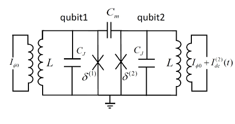
Figure 3: Circuit diagram of the capacitively-coupled phase qubits johnson1 . Here, two flux-biased Josephson phase qubits are coupled by the capacitance $C_{m}$. The time-dependent dc current $I^{(2)}_{dc}(t)$ is applied to the second qubit to generate the desirable Stark shift.

Suppose that the chirping current is sufficiently weak, such that the dynamics of each qubit is still safely limited within the subspace $\emptyset_{k}=\{|0_{k}\rangle,|1_{k}\rangle,|2_{k}\rangle\}$, $\sum_{l=0}^{2}|l_{k}\rangle\langle l_{k}|=1$. As a consequence, the circuit evolves within the total Hilbert space $\emptyset_{k}=\emptyset_{1}\otimes\emptyset_{2}$. Under the usual rotating-wave appropriation, $V_{1}$ and $V_{2}$ can be rewritten as

$$\tilde{V}_{1}(t)= \exp(itH_{01})\exp(itH_{02})V_{1}\exp(-itH_{01})\exp(-itH_{02})$$

$$= (\frac{2\pi}{\Phi_{0}})^{2}\frac{1}{\bar{C}_{m}}\Big{[}\sum|ij\rangle\langle ij|p_{ii}^{(1)}p_{jj}^{(2)}+\sum_{i\neq j}|ij\rangle\langle ji|p_{ij}^{(1)}p_{ji}^{(2)}$$

$$+|02\rangle\langle 11|p_{01}^{(1)}p_{21}^{(2)}\exp(-i\omega_{10}^{(1)}t)\exp(i\omega_{21}^{(2)}t)$$

$$+|11\rangle\langle 02|p_{10}^{(1)}p_{12}^{(2)}\exp(i\omega_{10}^{(1)}t)\exp(-i\omega_{21}^{(2)}t)$$

$$+|20\rangle\langle 11|p_{21}^{(1)}p_{01}^{(2)}\exp(i\omega_{21}^{(1)}t)\exp(-i\omega_{10}^{(2)}t)$$

$$+|11\rangle\langle 20|p_{12}^{(1)}p_{10}^{(2)}\exp(-i\omega_{21}^{(1)}t)\exp(i\omega_{10}^{(2)}t)\Big{]},$$ (37)

and

$$\tilde{V}_{2}(t) = \exp(itH_{02})V_{2}\exp(-itH_{02})$$ (38)

$$= -(\frac{\Phi_{0}}{2\pi})\frac{M}{L}I_{dc}^{(2)}(t)\sum|ij\rangle\langle ij|\delta_{jj}^{(2)},$$

with $i,j=0,1,2$, and $p_{ij}=-i\hbar\langle i|\frac{\partial}{\partial\delta}|j\rangle=-i\hbar p^{\prime}_{ij}$.

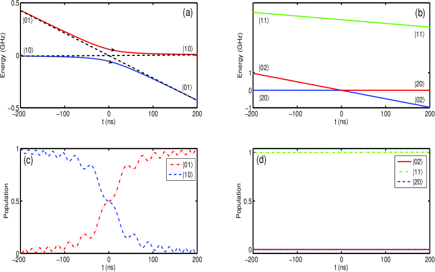
Figure 4: (Color online) Population evolutions in two capacitively-coupled qubits during the designed SCRAP: the Stark pulse is generated by applying the weak dc-current $I_{dc}(t)=\gamma t$ with $\gamma=2$ nA/ns. (a) Adiabatic passages and (c) population swap between$|01\rangle$ and $|10\rangle$. (b) The adiabatic paths and (d) the population evolution of the states in the subspace $\Im_{3}=\{|02\rangle,|11\rangle,|20\rangle\}$ versus passage time. Here, the system is initially prepared in the state $|11\rangle$. One can see that during the passage the population in this state is unchanged (dash-dotted green), and also the states $|02\rangle$ (solid red) and $|20\rangle$ (dashed blue) are kept to be unoccupied.

Under the condition that Stark shifts of the levels are relatively-weak, the matrix elements of momenta $p_{ij}^{(1)}=p_{ij}^{(2)}\equiv p_{ij}$. In fact, for the circuit with effective coupling coefficient $\zeta=0.0017$ considered here, our numerical calculations show that: $p^{\prime}_{00}=0.271,p^{\prime}_{11}=0.779,p^{\prime}_{22}=1.219,p^{\prime}_{01}=p^{\prime}_{10}=6.465,p^{\prime}_{02}=p^{\prime}_{20}=1.059,p^{\prime}_{12}=p^{\prime}_{21}=8.761$.

In the interaction picture, one can easily check that the dynamics of the system exists three invariant subspaces: (i) $\Im_{1}=\{|00\rangle\}$; (ii) $\Im_{2}=\{|01\rangle,|10\rangle\}$; and (iii) $\Im_{3}=\{|02\rangle,|11\rangle,|20\rangle\}$. The first subspace $\Im_{1}$ includes only one quantum state $|00\rangle$, the reduced Hamiltonian in this subspace reads $\tilde{H}_{1}(t)=E_{00}(t)|00\rangle\langle 00|$ with

$$E_{00}(t)=-\frac{\Phi_{0}}{2\pi}\frac{M}{L}I_{dc}^{(2)}(t)\delta_{00}^{(2)}+(\frac{2\pi}{\Phi_{0}})^{2}\frac{1}{\bar{C}_{m}}p_{00}^{(1)}p_{00}^{(2)}.$$

Certainly, if the system is initially prepared in the state $|00\rangle$, then it always populates in this state. This implies that we have the following evolution

$$|00\rangle\longrightarrow|00\rangle.$$

While, in the second subspace $\Im_{2}=\{a^{\prime}=|01\rangle,b^{\prime}=|10\rangle\}$, the corresponding Hamiltonian can be written as

$$\tilde{H}_{2}(t)=\left(\begin{array}[]{cc}0&\Omega_{a^{\prime}b^{\prime}}\\ \Omega_{b^{\prime}a^{\prime}}&\Delta_{b^{\prime}b^{\prime}}(t)\\ \end{array}\right),$$ (39)

with

$$\Omega_{a^{\prime}b^{\prime}} = \Omega_{b^{\prime}a^{\prime}}=(\frac{2\pi}{\Phi_{0}})^{2}\frac{1}{\bar{C}_{m}}p_{10}^{(1)}p_{10}^{(2)},$$

$$\Delta_{b^{\prime}b^{\prime}}(t) = \frac{\Phi_{0}}{2\pi}\frac{M}{L}I_{dc}^{(2)}(t)(\delta_{11}^{(2)}-\delta_{00}^{(2)}).$$

Returning to the Schrödinger picture, one can get the relevant adiabatic paths and the population evolutions (Fig. 4(a, c)). Of course, if the two qubits are exactly resonant, i.e., $\Delta_{b^{\prime}b^{\prime}}(t)=0$, Hamiltonian Eq. (39) will lead to a periodic swap of the populations between the states $|01\rangle$ and $|10\rangle$ bialczak with the period of $\hbar\pi/(2\Omega_{a^{\prime}b^{\prime}})$. Certainly, the efficiencies of these population transfers are sensitive to the evolution time $t$. In order to overcome these evolution-time sensitivities for implementing the desired swap operation, we apply an additional dc-current $I_{dc}^{(2)}(t)=\gamma t$ with $\gamma=2$ nA/ns to chirp the levels of the second qubit. If the system is initialized to be $|10\rangle$, then after the adiabatic passage (blue line in Fig. 4(a)), $|01\rangle$ can be populated. This relaxes the requirement of accurately designing the interaction time between the qubits. Yes, such a passage needs a longer time but it still could be finished within coherence time. In the subspace $\Im_{3}=\{a=|02\rangle,b=|11\rangle,c=|20\rangle\}$, the Hamiltonian expressed as

$$\tilde{H}_{3}(t)=\left(\begin{array}[]{ccc}E^{\prime}_{0}(t)&\Omega_{ab}\exp(-i\theta t)&\Omega_{ac}\\ \Omega_{ba}\exp(i\theta t)&E^{\prime}_{1}(t)&\Omega_{bc}\exp(i\theta t)\\ \Omega_{ca}&\Omega_{cb}\exp(-i\theta t)&E^{\prime}_{2}(t)\\ \end{array}\right).$$ (40)

Here

$$E^{\prime}_{i}(t) = -(\frac{\Phi_{0}}{2\pi})\frac{M}{L}I_{dc}^{(2)}(t)\delta_{jj}^{(2)}+(\frac{2\pi}{\Phi_{0}})^{2}\frac{1}{\bar{C}_{m}}p_{ii}^{(1)}p_{jj}^{(2)},$$

with $i\in\{0,1,2\},j=2-i$, and

$$\Omega_{ab} = \Omega_{ba}=(\frac{2\pi}{\Phi_{0}})^{2}\frac{1}{\bar{C}_{m}}p_{10}^{(1)}p_{12}^{(2)},$$

$$\Omega_{ac} = \Omega_{ca}=(\frac{2\pi}{\Phi_{0}})^{2}\frac{1}{\bar{C}_{m}}p_{20}^{(1)}p_{02}^{(2)},$$

$$\Omega_{cb} = \Omega_{bc}=(\frac{2\pi}{\Phi_{0}})^{2}\frac{1}{\bar{C}_{m}}p_{12}^{(1)}p_{10}^{(2)},$$

$$\theta = \frac{E_{1}-E_{0}}{\hbar}-\frac{E_{2}-E_{1}}{\hbar}=\omega_{10}-\omega_{21}.$$

Again, the corresponding Hamiltonian in the Schrödinger picture could be written as

$$\bar{H}_{3}(t)=\left(\begin{array}[]{ccc}E^{\prime}_{0}(t)-\hbar\theta&\Omega_{ab}&\Omega_{ac}\\ \Omega_{ba}&E^{\prime}_{1}(t)&\Omega_{bc}\\ \Omega_{ca}&\Omega_{cb}&E^{\prime}_{2}(t)-\hbar\theta\\ \end{array}\right).$$ (44)

The adiabatic paths and the corresponding population evolutions in this subspace are also illustrated in Fig. 4(b, d). As what we can see that, if the population initially resides in the state $|11\rangle$, then it always keeps in this state during the adiabatic passage designed for implementing the inversion between the $|10\rangle$ and $|01\rangle$. Since there is not any avoid crossing between the state $|02\rangle$ (or $|20\rangle$) and the state $|11\rangle$, the state $|02\rangle$ (or $|20\rangle$) should not be populated during the above passage.

IV Discussions and Conclusions

In summary, we showed that populations could be adiabatically transferred between the selected quantum states via SCRAP. Typically, these transfers are insensitive to the details of the applied pulses area. Based on these controllable population transfers, fundamental quantum gates and typical superposition states could be deterministically implemented. Our generic proposal is demonstrated by the experimentally-existing flux-biased Josephson phase qubits.

Our numerical results showed that, although the designed passages are required to be adiabatic, the single-qubit population inversion could still be finished within the duration as short as that of the usual $\pi$-pulse. However, as shown in Fig. (4) that the two-qubit logic gate operation with SCRAP technique takes relatively long time bialczak , e.g., about $300$ns required to finish the population inversion between $|01\rangle$ and $|10\rangle$. Thus, longer decoherence is required for the coupled superconducting circuits. We also investigated the influence of other levels on the designed adiabatic passages. It was shown that the population transfers are really limited between the selected levels and the leakages to other levels are negligible.

Note that the applied Stark pulse for chirping the levels should be sufficiently weak, compared with the original bias for defining the energy levels. For example, for realizing the above two-qubit operation, the maximal change ratios of the relevant transition frequencies (resulting from the applied Stark pulse) are estimated as $(\omega_{10}^{+}-\omega_{10})/\omega_{10}=-0.617\%$ and $(\omega_{10}^{-}-\omega_{10})/\omega_{10}=0.602\%$, respectively. Here, $\omega_{10}^{\pm}$ denote the transition frequencies between the states $|0\rangle$ and $|1\rangle$, due to the applying of a Stark current ( $\pm 400$ nA). Also, the applied Stark pulses vary the transition matrix elements very weak, such that the influences on the actions of the usual pump pulses could be negligible. As a consequence, the pump pulses could still resonantly interact with two selected levels.

APPENDIX

Schrödinger equation in the interaction picture reads

$$i\frac{\partial|\Psi(t)\rangle}{\partial t}=H^{\prime}_{int}(t)|\Psi(t)\rangle.$$ (A1)

In the new basis of $|\lambda_{-}(t)\rangle$ and $|\lambda_{+}(t)\rangle$,

$$|\Psi(t)\rangle=v_{-}(t)|\lambda_{-}(t)\rangle+v_{+}(t)|\lambda_{+}(t)\rangle.\\$$ (A2)

This induces that,

$$i\frac{\partial|\Psi(t)\rangle}{\partial t}=v_{-}(t)H^{\prime}_{int}(t)|\lambda_{-}(t)\rangle+v_{+}(t)H^{\prime}_{int}(t)|\lambda_{+}(t)\rangle$$

(A3)

Multiplying the above equation left with $\langle\lambda_{-}(t)|$, we get

$$i\frac{dv_{-}(t)}{dt} = v_{-}(t)\mu_{-}(t)-iv_{-}(t)\langle\lambda_{-}(t)|\frac{d}{dt}|\lambda_{-}(t)\rangle$$ (A4)

$$-iv_{+}(t)\langle\lambda_{-}(t)|\frac{d}{dt}|\lambda_{+}(t)\rangle$$

Similarly, multiplying Eq. (A3) left with $\langle\lambda_{+}(t)|$, we have

$$i\frac{dv_{+}(t)}{dt} = v_{+}(t)\mu_{+}(t)-iv_{+}(t)\langle\lambda_{+}(t)|\frac{d}{dt}|\lambda_{+}(t)\rangle$$ (A5)

$$-iv_{-}(t)\langle\lambda_{+}(t)|\frac{d}{dt}|\lambda_{-}(t)\rangle$$

This implies that

$$i\frac{d}{dt}\left(\begin{array}[]{c}v_{-}(t)\\ v_{+}(t)\\ \end{array}\right)=M_{1}\left(\begin{array}[]{c}v_{-}(t)\\ v_{+}(t)\\ \end{array}\right),$$ (A10)

with

$$M_{1}=\quad\quad\quad\quad\quad\quad\quad\quad\quad\quad\quad\quad\quad\quad\quad\quad\quad\quad\quad\quad\quad\quad\;$$

$$\left(\begin{array}[]{cc}\mu_{-}(t)-i\langle\lambda_{-}(t)|\frac{d}{dt}|\lambda_{-}(t)\rangle&-i\langle\lambda_{-}(t)|\frac{d}{dt}|\lambda_{+}(t)\rangle\\ -i\langle\lambda_{+}(t)|\frac{d}{dt}|\lambda_{-}(t)\rangle&\mu_{+}(t)-i\langle\lambda_{+}(t)|\frac{d}{dt}|\lambda_{+}(t)\rangle\end{array}\right).$$ (A12)

By using the expressions of $|\lambda_{+}(t)\rangle$ and $|\lambda_{-}(t)\rangle$ in Eqs. 8(a,b), we have

$$\langle\lambda_{-}(t)|\frac{d}{dt}|\lambda_{+}(t)\rangle=\frac{d\vartheta(t)}{dt}$$ (A13a)

$$\langle\lambda_{+}(t)|\frac{d}{dt}|\lambda_{-}(t)\rangle=-\frac{d\vartheta(t)}{dt}$$ (A13b)

$$\langle\lambda_{+}(t)|\frac{d}{dt}|\lambda_{+}(t)\rangle=0$$ (A13c)

$$\langle\lambda_{-}(t)|\frac{d}{dt}|\lambda_{-}(t)\rangle=0$$ (A13d)

So, $M_{1}$ can be simplified as

$$M^{\prime}_{1}=\left(\begin{array}[]{cc}\mu_{-}(t)&-i\frac{d\vartheta(t)}{dt}\\ i\frac{d\vartheta(t)}{dt}&\mu_{+}(t)\end{array}\right).$$ (A16)

Suppose that the condition

$$|\dot{\vartheta}(t)|\ll\mu_{+}(t)-\mu_{-}(t)$$ (A17)

is satisfied, then $M^{\prime}_{1}$ reduces to

$$M^{\prime\prime}_{1}=\left(\begin{array}[]{cc}\mu_{-}(t)&0\\ 0&\mu_{+}(t)\end{array}\right).$$ (A20)

Thus, the solutions of Eq. (A10) reads

$$\left(\begin{array}[]{c}v_{-}(t)\\ v_{+}(t)\\ \end{array}\right)=M_{2}\left(\begin{array}[]{c}v_{-}(0)\\ v_{+}(0)\\ \end{array}\right),$$ (A25)

with

$$M_{2}=\left(\begin{array}[]{cc}\exp(-i\int_{0}^{t}\mu_{-}(t^{\prime})dt^{\prime})&0\\ 0&\exp(-i\int_{0}^{t}\mu_{+}(t^{\prime})dt^{\prime})\\ \end{array}\right).$$ (A28)

Returning to the new (adiabatic) basis, the above adiabatic evolution solution takes the form

$$|\Psi(t)\rangle =v_{-}(0)\exp(-i\int_{0}^{t}\mu_{-}(t^{\prime})dt^{\prime})|\lambda_{-}(t)\rangle+$$ (A29)

$$v_{+}(0)\exp(-i\int_{0}^{t}\mu_{+}(t^{\prime})dt^{\prime})|\lambda_{+}(t)\rangle.$$

Here, the additional phases in adiabatic states can be regarded as the dynamical phases produced during the adiabatic passages.

Next, we show what an adiabatic condition should be satisfied by controlling Stark and pump pulses.

First, from the definition below Eq. (12),

$$\qquad\qquad\tan 2\vartheta(t) = \frac{\Omega(t)}{\Delta(t)}=\frac{2\tan\vartheta(t)}{1-\tan^{2}\vartheta(t)},$$ (A30)

we have

$$\frac{d}{dt}\tan 2\vartheta(t) = 2(1+\tan^{2}2\vartheta(t))\frac{d\vartheta}{dt}$$ (A31)

$$= \frac{\frac{d\Omega(t)}{dt}\Delta(t)-\Omega(t)\frac{d\Delta(t)}{dt}}{\Delta^{2}(t)},$$

and

$$\frac{d\vartheta(t)}{dt} = \frac{\frac{d\Omega(t)}{dt}\Delta(t)-\Omega(t)\frac{d\Delta(t)}{dt}}{2\Delta^{2}(t)(1+\tan^{2}2\vartheta(t))}$$ (A32)

$$= \frac{\frac{d\Omega(t)}{dt}\Delta(t)-\Omega(t)\frac{d\Delta(t)}{dt}}{2(\Delta^{2}(t)+\Omega^{2}(t))}.$$

The adiabatic condition Eq. (A17) implies that

$$\frac{1}{2}\left|\Omega(t)\frac{d\Delta(t)}{dt}-\Delta(t)\frac{d\Omega(t)}{dt}\right|\ll\left(\Delta^{2}(t)+\Omega^{2}(t)\right)^{3/2}.$$ (A33)

Therefore, smooth pulses, long interaction time, and large Rabi frequency and detuning are needed to satisfy the desirable adiabatic condition.

References

• (1) Y. Makhlin, G. SchΓΆn, and A. Shnirman, Rev. Mod. Phys. 73, 357 (2001).
• (2) J. Q. You, and F. Nori, Phys. Today 58, 42 (2005).
• (3) J. Clarke, and F. K. Wilhelm, Nature(London) 453, 1031 (2008).
• (4) G. Wendin, and V. S. Shumeiko, arXiv:cond-mat/0508729.
• (5) M. H. Devoret, and J. M. Martinis, Quant. Info. Proc. 3, 163-203 (2004).
• (6) Y. Nakamura, Y. A. Pashkin, and J. S. Tsai, Nature(London) 398, 786 (1999).
• (7) J. R. Friedman, V. Patel, W. Chen, S. K. Tolpygo, and J. E. Lukens, Nature(London) 406, 43 (2000).
• (8) J. E. Mooij, T. P. Orlando, L. Levitov, L. Tian, C. H. van der Wal, and S. Lloyd, Science 285, 1036 (1999).
• (9) J. M. Martinis, S. Nam, and J. Aumentado, Phys. Rev. Lett. 89, 117901 (2002).
• (10) R. W. Simmonds, K. M. Lang, D. A. Hite, S. Nam, D. P. Pappas, and J. M. Martinis, Phys. Rev. Lett. 93, 077003 (2004).
• (11) A. J. Berkley, H. Xu, R. C. Ramos, M. A. Gubrud, F. W. Strauch, P. R. Johnson, J. R. Anderson, A. J. Dragt, C. J. Lobb, and F. C. Wellstood, Science 300, 1548 (2003).
• (12) J. Koch, T. M. Yu, J. Gambetta, A. A. Houck, D. I. Schuster, J. Majer, A. Blais, M. H. Devoret, S. M. Girvin, and R. J. Schoelkopf, Phys. Rev. A 76, 042319 (2007).
• (13) V. E. Manucharyan, J. Koch, L. I. Glazman, and M. H. Devoret, Science 326, 113 (2009).
• (14) D. Vion, A. Aassime, A. Cottet, P. Joyez, H. Pothier, C. Urbina, D. Esteve, and M. H. Devoret, Science 296, 886 (2002).
• (15) P. J. Leek, J. M. Fink, A. Blais, R. Bianchetti, M. GΓΆppl, J. M. Gambetta, D. I. Schuster, L. Frunzio, R. J. Schoelkopf, and A. Wallraff, Science 318, 1889 (2007).
• (16) L. F. Wei, Y. X. Liu, and F. Nori, Phys. Rev. B 72, 104516 (2005).
• (17) M. Ansmann, H. Wang, R. C. Bialczak, M. Hofheinz, E. Lucero, M. Neeley, A. D. O’Connell, D. Sank, M. Weides, J. Wenner, A. N. Cleland, and J. M. Martinis, Nature(London) 461, 504 (2009).
• (18) K. Bergmann, H. Theuer, and B. W. Shore, Rev. Mod. Phys. 70, 1003 (1998).
• (19) L. P. Yatsenko, B. W. Shore, T. Halfmann, K. Bergmann, and A. Vardi, Phys. Rev. A 60, R4237 (1999).
• (20) A. A. Rangelov, N. V. Vitanov, L. P. Yatsenko, B. W. Shore, T. Halfmann, and K. Bergmann, Phys. Rev. A 72, 053403 (2005).
• (21) M. Oberst, H. MΓΌnch, and T. Halfmann, Phys. Rev. Lett. 99, 173001 (2007).
• (22) E. A. Shapiro, V. Milner, C. Menzel-Jones, and M. Shapiro, Phys. Rev. Lett. 99, 033002 (2007).
• (23) T. Rickes, L. P. Yatsenko, S. Steuerwald, T. Halfmann, B. W. Shore, N. V. Vitanov, and K. Bergmann, J. Chem. Phys. 113, 534 (2000).
• (24) Z. Kis, and E. Paspalakis, Phys. Rev. B 69, 024510 (2004).
• (25) J. Siewert, T. Brandes, and G. Falci, Phys. Rev. B 79, 024504 (2009).
• (26) K. H. Song, S. H. Xiang, Q. Liu, and D. H. Lu, Phys. Rev. A 75, 032347 (2007).
• (27) K. Y. Xia, M. Macovei, J. Evers, and C. H. Keitel, Phys. Rev. B 79, 024519 (2009).
• (28) L. F. Wei, J. R. Johansson, L. X. Cen, S. Ashhab, and F. Nori, Phys. Rev. Lett. 100, 113601 (2008).
• (29) K. B. Cooper, M. Steffen, R. McDermott, R. W. Simmonds, S. Oh, D. A. Hite, D. P. Pappas, and J. M. Martinis, Phys. Rev. Lett. 93, 180401 (2004).
• (30) R. C. Bialczak, M. Ansmann, M. Hofheinz, E. Lucero, M. Neeley, A. D. O’Connell, D. Sank, H. Wang, J. Wenner, M. Steffen, A. N. Cleland and J. M. Martinis, Nat. Phys. 6, 409 (2010).
• (31) J. M. Martinis, Quant. Info. Proc. 8, 81-103 (2009).
• (32) M. Ansmann, Ph.D. thesis, UCSB, 2009.
• (33) J. Clarke, A. N. Cleland, M. H. Devoret, D. Esteve, and J. M. Martinis, Science 239, 992 (1988).
• (34) M. Steffen, J. M. Martinis, and I. L. Chuang, Phys. Rev. B 68, 224518 (2003).
• (35) P. R. Johnson, W. T. Parsons, F. W. Strauch, J. R. Anderson, A. J. Dragt, C. J. Lobb, and F. C. Wellstood, Phys. Rev. Lett. 94, 187004 (2005).
• (36) M. Steffen, M. Ansmann, R. C. Bialczak, N. Katz, E. Lucero, R. McDermott, M. Neeley, E. M. Weig, A. N. Cleland, and J. M. Martinis, Science 313, 1423 (2006).
• (37) P. R. Johnson, F. W. Strauch, A. J. Dragt, R. C. Ramos, C. J. Lobb, J. R. Anderson, and F. C. Wellstood, Phys. Rev. B 67, 020509(R) (2003).
• (38) A. G. Kofman, Q. Zhang, J. M. Martinis, and A. N. Korotkov, Phys. Rev. B 75, 014524 (2007).