Stability of Cloud Orbits in the Broad Line Region of Active Galactic Nuclei

Abstract

We investigate the global dynamic stability of spherical clouds in the Broad Line Region (BLR) of Active Galactic Nuclei (AGN), exposed to radial radiation pressure, gravity of the central black hole (BH), and centrifugal forces assuming the clouds adapt their size according to the local pressure. We consider both, isotropic and anisotropic light sources. In both cases, stable orbits exist also for very sub-Keplerian rotation for which the radiation pressure contributes substantially to the force budget. We demonstrate that highly eccentric, very sub-Keplerian stable orbits may be found. This gives further support for the model of Marconi et al. (2008), who pointed out that black hole masses might be significantly underestimated if radiation pressure is neglected. That model improved the agreement between black hole masses derived in certain active galaxies based on BLR dynamics, and black hole masses derived by other means in other galaxies by inclusion of a luminosity dependent term. For anisotropic illumination, energy is conserved for averages over long time intervals, only, but not for individual orbits. This leads to Rosetta orbits that are systematically less extended in the direction of maximum radiation force. Initially isotropic relatively low column density systems would therefore turn into a disk when an anisotropic AGN is switched on.

1 Introduction

Recently, the BLR has received much attention, because the line widths, in combination with the size of the region, measured for example by reverberation mapping, allows a determination of the mass of the central super-massive black hole (e.g. Bentz et al. 2009; Netzer 2009), which is essential if one wants to place AGN in the context of general galaxy evolution. From such studies, one finds that AGN generally have normal sized black holes, as expected for the size of their host galaxy, and that most galaxies must have been active for one or more times in their life. The measurement of the black hole mass is affected by the relative importance of radiation pressure and gravity, which should dominate the force budget. This is connected to the properties of individual BLR clouds and the dynamical configuration of the system (Marconi et al. 2008).

The BLR is a standard AGN ingredient (e.g. Osterbrock 1988; Peterson 1997; Netzer 2008): It is located inside the obscuring torus, above and below the accretion disk, and at a distance of fractions of a parsec from the super-massive black hole. The line emission is powered by photoionisation by a broad-band continuum due to the innermost parts of the accretion disk. Photoionisation also governs the thermodynamics of these clouds: They have a stable equilibrium temperature of order $10^{4}$ K, independent of their locations. The critical densities of observed and suppressed emission lines and pressure equilibrium considerations (Ferland & Elitzur 1984) constrain the number densities in the clouds to $n_{\mathrm{cl}}=10^{10\pm 1}$ cm^-3. Signatures from partially ionised zones are typically observed. Therefore, the Strömgren depth is a lower limit of the cloud size. An upper limit may be found by requiring the lines to be smooth, which demands a certain minimum on the number of individual entities. This results in cloud sizes of about $r_{\mathrm{cl}}=10^{12\pm 1}$ cm (Laor et al. 2006, and references therein). In agreement with this, detailed photoionisation models (Kwan & Krolik 1981) constrain the column densities to $N_{\mathrm{cl}}>10^{22}$ cm^-2. Because BLR clouds are optically thick, high ionisation lines are produced only by the illuminated surface of the clouds. In such lines, one observes generally the far side of the BLR, wherefore outflows manifest themselves as redshifts, inflows as blueshifts.

Much information has also been gathered on the dynamical state of the BLR. Inclination matters: the statistics of line widths excludes Keplerian rotation in a flat disk, but is instead consistent with a thick disk configuration with $v/\sigma\approx 2.5$, where $v$ is the rotational velocity and $\sigma$ the turbulent one (Osterbrock 1978). For radio-loud AGN, the ratio of core to lobe power correlates with the width of the broad lines in the sense that the systems observed at a line-of-sight close to the jet axis have the narrower lines (Wills & Browne 1986). This finding was confirmed by Jarvis & McLure (2006). They find that the average line width of flat spectrum radio sources, which are seen more face on, have narrower emission lines by about 30% than steep spectrum radio sources. Spectropolarimetry of type 2 objects, where the BLR is hidden by a dusty torus, has revealed hidden BLRs in polarised light, which established the orientation unification scenario (Antonucci 1993). In these objects, the BLR emission is scattered by a polar region above the BLR. The polarisation angle is perpendicular to the system axis, defined by the radio (Smith et al. 2004) or UV/blue (Borguet et al. 2008) emission. The same authors find a preferentially parallel orientation for type 1 objects, which provide an unobscured view towards the BLR. This finding is explained by an equatorial scattering region, much closer to the BLR. Where observed (type 1 objects), the latter dominates the polarised emission. The equatorial scatterer is in fact very close to the BLR and provides unambiguous evidence for a disk-like configuration of the BLR (Smith et al. 2005): Approaching and receding parts of the BLR-disk are seen at slightly different angles by the equatorial scatterer. This produces a noticeable difference in polarisation angle for the blue and red parts of the line. This, and other characteristics, has been observed by Smith et al. (2004, 2005) for a sample of Seyfert galaxies. They find a continuum of polarisation properties: Zero polarisation for near pole on objects, where the different contributions by equatorial scatterers in various directions cancel each other; wavelength dependent parallel polarisation for intermediate inclination type 1 objects, where parts of the BLR and the equatorial scattering region are attenuated by the obscuring torus; and perpendicular polarisation for type 2 objects. Other evidence pointing to a disk-like nature of the BLR comes from the existence of objects with double peaked broad lines indicative of Keplerian motion (Eracleous & Halpern 2003, 12% in their sample), while the majority of single peaked objects allows for a hidden disk component, if the inclination is small, and the contribution of the flattened part is not too strong (Bon et al. 2009). These findings suggest that the dominant contribution to the BLR kinematics is Keplerian rotation, followed by a turbulent component. There is also evidence for radial motion: There are examples in the literature for bulk outflows, as measured by spectropolarimetry (Young et al. 2007, and references therein). Velocity resolved reverberation mapping confirms the dominant Keplerian motions, but additionally finds evidence for bulk inflow and outflow in individual objects (e.g. Done & Krolik 1996; Ulrich & Horne 1996; Kollatschny 2003; Bentz et al. 2008, 2009; Denney et al. 2009). Gaskell (2009) interprets the combined evidence of velocity resolved reverberation mapping as strong evidence that the radial part of the kinematics is dominated by inflow.

Radiation pressure due to the central parts of the accretion disk is generally assumed to be significant in the BLR (e.g. Blumenthal & Mathews 1975; Mathews 1986; Marconi et al. 2008; Netzer 2009). Since the dependence on distance to the light emitter is an inverse square law, like for gravity, the effect of radiation pressure support is to reduce the apparently measured mass of the black hole, based on BLR kinematics. Recently, it has been under debate, how strong this effect was (Marconi et al. 2008, 2009; Netzer 2009; Netzer & Marziani 2010), especially in the case of NLS1 galaxies. It is interesting to ask in this context, which cloud orbits would be stable against small perturbations, and also, which ones are compatible with the spectropolarimetric results. In the following we perform such an analysis.

We present the cloud orbit analysis in sect. 2, discuss our finding in sect. 3 and summarise our conclusions in sect. 4.

2 Dynamical stability analysis

We carry out the analysis for both, an isotropic light source, and a light source with a $\cos\theta$ dependence for the luminosity, where $\theta$ is the polar angle. The latter case should be more realistic, as it is the expected angular distribution for the luminosity of a thin accretion disk.

2.1 Isotropic light source

For optically thick, spherical clouds of constant mass $m$ and central column density $N$, without internal structure, the force equation in spherical polar coordinates reads:

$$F=\frac{GM_{\mathrm{BH}}m}{R^{2}}\left(\frac{3l}{2\sigma_{\mathrm{T}}N}+V^{2}-1\right)\,,$$ (1)

where $\sigma_{\mathrm{T}}$ is the Thomson cross section, $l$ the luminosity in Eddington units, $V$ the rotational velocity in Kepler units and $M_{\mathrm{BH}}$ the mass of the black hole.

Dynamical equilibrium, corresponding to circular orbits, is reached for a column density of:

$$N=\frac{3l}{2\sigma_{\mathrm{T}}(1-V^{2})}\,.$$ (2)

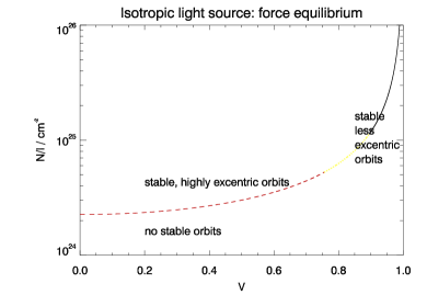
Figure 1: Dynamical equilibrium column density over luminosity in Eddington units against rotation velocity in Kepler units for an isotropic light source. The red, dashed part of the line corresponds to a maximum of the effective potential for reasonable choices of the parameter $s$ ($s>1$) that characterises the pressure profile. Stable orbits are still found in this case, but are highly eccentric, and are found above the red line. The yellow, dotted part corresponds to a stable minimum for certain values of $s$. The solid, black region is always a minimum of the effective potential, provided $s<3$, and therefore allows for orbits with low eccentricity, which scatter around the line. See text for more details.

For a large range of rotational velocities $V$, this is of order $10^{24}\,l$ cm^-2 (compare Fig. 1).

To assess dynamical stability, we now consider perturbations to circular orbits. Following Netzer (2008), we assume a confining inter-cloud medium with a pressure profile of $p(R)\propto R^{-s}$. The sound crossing time through a BLR cloud is of order weeks, whereas the orbiting period is many years. We therefore assume the clouds to adjust their radius instantaneously to any change in external pressure. A change in the clouds’ cross section alters the amount of radiation received and hence the radiation pressure support. Clouds will be dynamically stable, if an increase (decrease) in orbital radius $R$ leads to a net inward (outward) force, i.e. a position above (below) the equilibrium line in Fig. 1. We proceed to calculate the perturbed locations in the $N/l-V$-diagram.

We first consider a spherically symmetric cloud initially in a circular orbit at distance $R$ to the black hole. Since the temperature is kept constant by photoionisation, a change in distance by $\Delta R>0$ will result in a change of the particle density by $n(R+\Delta R)=n(R)[(R+\Delta R)/R]^{-s}$. This results in a change of the column density:

$$N(R+\Delta R)=N(R)(1+\Delta R/R)^{-2s/3}\,.$$ (3)

The corresponding change in orbital velocity for angular momentum conserving perturbations is:

$$V(R+\Delta R)=V(R)(1+\Delta R/R)^{-1/2}\,.$$ (4)

The perturbed cloud will receive a restoring force, if:

$$N(R+\Delta R)>\frac{3l}{2\sigma_{\mathrm{T}}(1-V(R+\Delta R)^{2})}\,.$$ (5)

It may be shown by a few lines of algebra that this condition may be fulfilled only if

$$V^{2}>V_{\mathrm{c}}^{2}=\frac{1}{1+\frac{3}{4s}}\,.$$ (6)

The analogous derivation for $\Delta R<0$ leads to the same result. If the rotational velocity is below this value, positive perturbations to $R$ lead to ejection. Negative ones lead to highly eccentric orbits. We show this by considering the effective potential $V_{\mathrm{eff}}$. Inserting eqs. (3) and (4) into eq. (1), and defining $R_{0}$ to be a fiducial distance to the black hole where eq. 2 holds, with $N(R_{0})=N_{0}$, $V(R_{0})=V_{0}$ and $x=R/R_{0}$, we derive:

$$V_{\mathrm{eff}}(x) = \frac{GM_{\mathrm{BH}}m}{R_{0}}\left[-(1-V_{0}^{2}){\cal R}(x)+\frac{V_{0}^{2}}{2x^{2}}-\frac{1}{x}\right]$$ (7)

$${\cal R}(x) = \left\{\begin{array}[]{ll}\log(x)&s=3/2\\ \frac{3}{2s-3}x^{2s/3-1}&s\neq 3/2\end{array}\right.$$ (10)

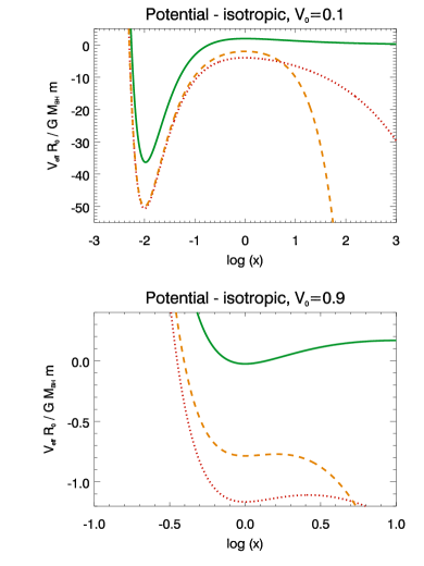
Figure 2: Normalised effective potential against normalised distance between cloud and black hole for a rotation velocity of $V_{0}=0.1$ (top) and $V_{0}=0.9$ (bottom) normalised to the Kepler value at $R=R_{0}$ ($x=1$) for the case of isotropic illumination. In each case, the solid green (dotted red, dashed yellow) line is for $s=1$ (2,3).

The effective potential is displayed in Fig. 2. In agreement with the preceding discussion, there is an extremum at $x=1$, whose character depends on $V_{0}$: For $V_{0}>V_{\mathrm{c}}$ (compare eq. 6), it is a minimum. Stable bound orbits with small radial motions may be found in this case. For $V_{0}<V_{\mathrm{c}}$, the extremum at $x=1$ is a maximum. In this case, their exists a minimum further in. The equations can be solved easily analytically for $s=0$, $3/2$ and 3. For $s=3/2$, the second extremum is at:

$$x_{\mathrm{e2}}=\frac{V_{0}^{2}}{1-V_{0}^{2}}\,.$$ (11)

This extremum is a minimum for $V_{0}<V_{\mathrm{c}}$. We have verified numerically that for all $1<s<3$, $x_{\mathrm{e2}}$ is very close to the value of the $s=3/2$-case, for $V_{0}<V_{\mathrm{c}}$. Again, stable bound solutions may be found. If a cloud is very deep in that potential well, the orbits are close to circular, and dominated by rotation. The average column density and rotation velocity for such an orbit are much higher than the values at $R_{0}$. Such orbits are therefore effectively on the stable, solid black part of the equilibrium curve in Fig. 1. Orbits with total energy close to the potential energy at the maximum will follow highly eccentric orbits, with predominantly radial kinematics. For a significant fraction of their orbital period, they have indeed low column densities and rotational velocities, corresponding to the region above the red dashed part of the line in Fig. 1.

2.2 Anisotropic light source

The luminosity in Eddington units for a geometrically thin accretion disk is a function of the polar angle and is given by $2l|\cos\theta|$, where $l$ is the total luminosity of the source in Eddington units. The force is still central and therefore, angular momentum is conserved. The orbits are planar. Any particular orbital plane may be characterised by a polar angle $\theta_{\mathrm{o}}$. We define the direction of the maximum elevation above the equatorial plane to have an azimuth of $\phi=0$. A cloud will then have maximum radiation pressure support at $\phi=0$ and $\phi=\pi$, and no radiation pressure support at $\phi=\pi/2$ and $\phi=3\pi/2$, when passing the equatorial plane. Geometrical considerations result in: $\cos\theta=\cos\phi\,\cos\theta_{\mathrm{o}}$. Using this, and eqs (1), (3) and (4), results in the following total force equation:

$$F=\frac{GM_{\mathrm{BH}}m}{R^{2}}\left(\frac{3l|\cos\phi\,\cos\theta_{\mathrm{o}}|}{\sigma_{\mathrm{T}}N_{0}x^{-2s/3}}+V_{0}^{2}x^{-1}-1\right)\,,$$ (12)

where $x=R/R_{0}$, $R(\phi=\pi/2)=R_{0}$, $N(\phi=\pi/2)=N_{0}$. The azimuthal velocity at $\phi=\pi/2$ in Kepler units is denoted by $V_{0}$. Because of the $\phi$-dependence, the force is no longer conservative. We therefore expect the total energy and hence also the major axis of the orbits to grow or diminish, depending on whether the cloud moves predominantly with or against the radiation flux.

First, we consider the force free locations, which are useful to understand the general structure of the allowed orbits. In the standard treatment of the Kepler problem, bound orbits require the existence of a local minimum of the effective potential. The elliptic orbits are then oscillating around this minimum. The forces in this case vanish, of course, at the minimum. Away from the minimum, there is an effective restoring force. If the total energy is too large, the object can reach a region where the effective force is away from the equilibrium point, and may escape. A similar analysis may be done for the present problem: Making the definition:

$$a=\frac{3l\cos\theta_{\mathrm{o}}}{\sigma_{\mathrm{T}}N_{0}}\,,$$ (13)

we find the condition for force-free lines:

$$a|\cos\phi|=x^{2s/3}(1-V_{0}x^{-1})\,.$$ (14)

A force-free line in the orbit plane is defined by specifying the parameters $a$ and $s$. Since there is no radiation force in the equatorial plane, force-free lines require $V_{0}=1$. We show $x$ as a function of $a\,|\cos\phi|$ for different values of $s$ in Fig. 3.

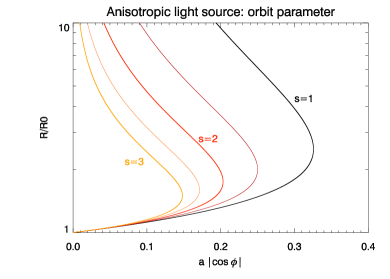
Figure 3: Force-free lines for the case of the anisotropic light source: normalised distance between cloud and black hole versus $a|\cos\phi|$ for different values of the pressure distribution index $s$. The force is outward to the right of each curve, and inward on the left side. Around the lower branch of each line, the force is always restoring. Stable orbits are therefore expected in this region of the parameter space. If the cloud has low enough column density, a too large part of the orbit will be right of the force-free line, where the force is always outward, leading to ejection of the cloud.

Each curve is characterised by a rightmost value, $a\,|\cos\phi|=a_{\mathrm{max}}$, where the upper branches with negative slopes and the lower branches with positive slopes meet. The force is restoring in the vicinity of the lower branches with positive slope. Therefore, if $a\,\cos\phi<a_{\mathrm{max}}\forall\phi$ , we expect bound orbits to exist. We do not necessarily expect bound orbits if $a\,\cos\phi$ exceeds this value for some fraction of the orbit. From eq. (14), we find:

$$a_{\mathrm{max}}=\frac{3}{2s}\left(\frac{1}{1+\frac{3}{2s}}\right)^{\frac{2s}{3}+1}\,.$$ (15)

For $s=2$ (1,3), $a_{\mathrm{max}}$ evaluates to 0.20 (0.33, 0.15). Consequently, there is a $\theta_{\mathrm{o}}$ and $l$-dependent critical column density, above which bound orbits should be found:

$$N_{0}\gtrsim 7\times 10^{23}\mathrm{cm}^{-2}\frac{l}{0.1}\frac{\cos\theta_{\mathrm{o}}}{0.5}\frac{0.33}{a_{\mathrm{max}}}\,.$$ (16)

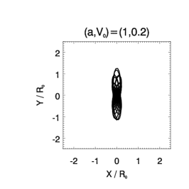
                      $(a,V_{0})=(0.1,1.1)$                                                            $(a,V_{0})=(1,0.2)$

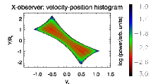
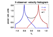
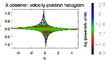
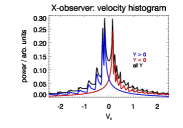
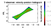
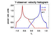
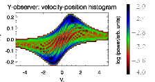
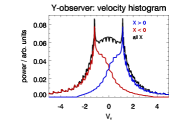
Figure 4: Position and kinematic data for three example orbits for the anisotropic case. Radiation pressure support is maximal on the X-axis, and zero on the Y-axis. We have integrated for 100 orbits, for the bound cases. The simulations are converged with regard to the timestep. Top row: orbit shapes in orbit plane. The orbits are similar to precessing Kepler-ellipses. Because of the non-conservative nature of the potential, they grow and shrink periodically, with a period of $\pi$. This leads to Rosetta shapes, which are compressed in the direction of maximum radiation support. The set of four plots on the lower left shows kinematic information for the $(a,V_{0})=(0.1,1.1)$ simulation. Here we assume that a cloud emits radiation on the illuminated side facing the centre. We calculate the fraction of that surface seen by respective observers. The emission is further proportional to the current cloud surface and the time interval. The top row relates to an observer in $-X$-direction (X-observer), the bottom one to an observer in $-Y$-direction (Y-observer). The left column shows position-velocity diagrams, the right one the emission at a given velocity (black) and separately for negative (red) and positive (blue) values of the respective complementary coordinate. The emission of the two peaks at about half the Kepler velocity is easily discerned. The lower right set of four plots shows the same for the run with $(a,V_{0})=(1,0.2)$. The emission occurs predominantly at smaller velocities. In velocity space, emission from the sides with positive coordinates still has little overlap with the emission from the other sides. Colour scales are cut at reasonable values, as indicated at the individual colour bars. Velocity is given in units of the local Kepler velocity at the initial cloud position $R_{0}$.

Similarly as in the isotropic case, we also find bound, but highly eccentric orbits for low column densities and rotation velocities: We show this by numerical integration of some example orbits (Fig 4). Our reference in the following is a Cartesian coordinate system with coordinates $X$ and $Y$ defined in the orbital plane. The $Y$-axis is taken to be the intersection between the orbital and the equatorial plane. We use $s=2$ and start the clouds at $\phi=\pi/2$, i.e. where the orbital plane meets the equatorial plane (positive $Y$-axis in Fig 4), with certain values for $a$ and $V_{0}$. For $(a,V_{0})=(0.1,1.1)$, we expect a stable bound orbit despite the super-Keplerian initial velocity, since $a$ is in the stable regime. This is indeed the case (Fig. 4, top left). For $(a,V_{0})=(1,1)$, we expect ejection, since $a$ is in the unstable regime and the comparatively high velocity corresponds to a positive radial perturbation. Again, this is what we find (Fig. 4, top middle). For $(a,V_{0})=(1,0.2)$, we expect highly eccentric orbits. This is confirmed by the numerical integration (Fig. 4, top right). Here, the non-conservative nature of the potential is most apparent: The cloud gains energy, when moving outwards. But since it advances in azimuth, it does not get back the same amount on the way inwards. However, on average over many orbits, the contributions cancel each other.

In order to obtain kinematic information, we also recorded the emission measure, $e$, of the cloud into a certain direction during the integration, together with the current position and velocity. At each time $t$, it is calculated as:

$$e(t)=A(\phi)\,\mathrm{d}t\,R^{2s/3-2}\,,$$

where $A(\phi)$ is the fraction of the illuminated cloud surface seen by the observer. We take only the side facing the AGN as line emitting region, as appropriate for an optically thick line. The current time step interval is denoted by $\mathrm{d}t$, and the radial dependence is due to the change of the cloud size and radiation flux with distance to the centre. We place two observers at large negative $X$ and $Y$ values, respectively. At each timestep, we project the clouds velocity along the respective lines-of-sight. $e(t)\,\mathrm{d}t$ is then added to the corresponding bins of line-of-sight velocity and transverse position in order to create a two-dimensional emission-weighted histogram.

For the bound orbits, these velocity resolved emission-weighted histograms are shown in Fig 4. A priori, one might expect a broader signal for the low $a$ (high column density) case with well separated emission peaks near the positive and negative Kepler velocity, and a narrower signal for the high $a$ (low column density) case. This is indeed what we find. For $(a,V_{0})=(0.1,1.1)$, the peak of the emission is at $\pm\approx 50$ per cent of the Keplerian velocity at $R_{0}$. For $(a,V_{0})=(1,0.2)$, the orbits get very anisotropic in real space as well as in velocity space. An observer in the $-X$-direction would see two peaks at around $\pm 0.15$ times the Kepler velocity at $R_{0}$, close to the initially imposed one. Here, the outermost locations of the orbit dominate the emission due to the longer time spent there. An observer in the $-Y$-direction would see the two peaks at around $1.2$ times the Kepler value, because from this point of view, the orbits are much narrower. If there was an ensemble of such clouds with the angular momentum vector randomly rotated around the symmetry axis of the system, but otherwise identical, the signal at low velocity would dominate, as the emissivity at the slower peak is about three times higher. For an observer who would see the orbital plane at some inclination, the apparent velocities would be somewhat below these values. Since spectropolarimetric observations are able to resolve the BLR in many objects, we have also separated the emission that comes from the positive part of the transverse axis from the one of the opposite side. As one might have expected, the emission from the two sides is well separated in velocity space, in both cases. Remarkably, for the emission from a given side, the $(a,V_{0})=(1,0.2)$ cloud shows about ten percent of the peak emission of the opposite side at the location of the peak of the opposite side. In contrast, for the cloud with $(a,V_{0})=(0.1,1.1)$, the emission of a given side drops to zero at the peak of the other side.

3 Discussion

We have shown that pressure confined clouds at any sub-Keplerian rotational velocity may exist in stable dynamical equilibrium in the BLR. Given the significant evidence for a gravitationally bound, flattened, but still of considerable thickness, and disk-like geometry for the BLR (compare sect. 1), it is reasonable to require a stable dynamical equilibrium for the line-emitting clouds.

An essential ingredient for the model is the behaviour of the pressure of the inter-cloud material with radius: A reasonable assumption for the inter-cloud component is an Advection Dominated Accretion Flow (ADAF, e.g. Narayan & Yi 1994; Yuan, Ma, & Narayan 2008). A nearly hydrostatic solution is included in the ADAF models for the limit of low accretion rates. For this type of solutions, the power law index for the pressure $s$ is between two and three. Outflow solutions have also been considered in the literature. Königl & Kartje (1994) find $1<s<1.5$. Therefore, $s$ should be between one and three (similar results are obtained by Rees, Netzer, & Ferland 1989).

We have considered an isotropic and an anisotropic light source as appropriate for an accretion disk. The former is usually implied in the literature. For the isotropic case, the force is central (i.e. conserves angular momentum) and conservative. We find an equilibrium relation between column density, luminosity of the AGN and rotational velocity. We show by direct stability analysis that only for the part of that relation with high rotational velocities a cloud would encounter a restoring force for small radial perturbations. However, by analysis of the effective potential, we show that stable orbits may be found also for low rotational velocities and column densities slightly above the equilibrium curve given by eq. (2). However, the character of these orbits changes: while high column densities (corresponding to close to Keplerian rotation) allow for even circular orbits, low column density clouds require highly eccentric ones.

For anisotropic illumination, the force is still central, and therefore angular momentum conserving, but it is no longer conservative. Therefore, as the orbits precess, there is now the additional feature that they gain and loose total energy, which is exchanged with the radiation field. This is evident from the periodic change of the major axis of the orbits. We show that the time averaged signal of such a cloud would also be very anisotropic. If one would consider many such clouds with randomly rotated angular momentum vector around the axis of symmetry, the stronger emission from further out would dominate. In our example, this produces a peak in emission at a small fraction of the Keplerian velocity with a similar FWHM. More important, the emission contributions from the two sides of the accretion disk are kinematically clearly distinct. This would therefore probably still be compatible with the spectropolarimetric results. More detailed comparisons using realistic cloud samples have to be done in order to decide if the dispersion would be low enough to fit with all the available data. This is however beyond the scope of this article.

Cloud column density and rotation velocity in the anisotropic case are still related by eq. (2) (also Fig. 1), when orbit averaged values are used. Therefore, it is well possible to observe arbitrarily low rotation velocities for cloud column densities of order $10^{23}(l/0.1)$ cm^-2, confirming the results of Marconi et al. (2008).

Interestingly, it has turned out that for the anisotropic case, the orbits are less extended in the direction of the strongest radiative force. This might first appear counter-intuitive, but is readily explained if one considers that the radiative force adds energy to the orbit, as long as the motion is outward, but brakes down the cloud, when it moves inward. If the major orbit axis coincides with the direction of maximum radiation force, the contributions nearly cancel, whereas one may get positive changes when the major axis has advanced past that direction. Energy losses are expected, when the major axis has not yet reached the maximum force direction.

If the column densities are not too high, the radiation field favours a disk configuration: Consider an initially isotropic ensemble of clouds with relatively low column densities, comparable to the one given in eq. (16), and a broad distribution of angular momenta. Due to angular momentum conservation, each cloud orbits the black hole in a particular orbital plane on an elliptical orbit. Once an anisotropic AGN is switched on, we may assign an $a$ value to each cloud. Because $a\propto\cos(\theta_{\mathrm{o}})$, clouds at low polar angle (closer to the symmetry axis of the emission of the central accretion disk) have greater $a$ values. If this $a$ value is too large, the high angular momentum clouds will be ejected. For the remaining clouds at low polar angle, the major axis of their orbits will shrink when it points towards higher latitudes on their course of precession. In Fig 4 we have demonstrated this effect. The result will be a disk-like BLR. For column densities much higher than the one given in eq. (16), the orbits are less affected by radiation pressure. For such clouds, the BLR would therefore not be constrained to have a disk or other geometry by these dynamic considerations. It may or may not be in a disk configuration for other reasons. The critical column density is of the order $10^{24}$ cm^-2 for common luminosities of ten per cent of the Eddington value, which is rather large compared to observational constraints (compare references in sect. 1). One might therefore generally expect this effect to be significant in many BLRs.

The detailed mixture of orbits is of course very hard to predict. Since the cloud mass is unimportant for the acceleration of the cloud, we expect clouds of a wide range of masses, with the column density adjusting according to the cloud’s position in phase space. Some BLR clouds might have been born in situ (e.g. Perry & Dyson 1985). If the clouds would have come from further out, an interaction would be required to reach the bound orbits. This might favour eccentric orbits. The mixture of orbits will determine the observed velocity structure.

Pressure confined spherical clouds as used in this analysis, suffer from shearing by differential radiative forces due to the varying column density from the cloud’s rim to it’s centre (Mathews 1986). For our parameters one would expect complete disruption after about a hundredth of an orbital period. This issue is common to this class of cloud model (compare e.g. Rees et al. 1989), and has not been solved so far. Possible ideas to stabilise the clouds include magnetic fields and a more favourable geometry (e.g. Netzer 2008).

4 Conclusions

We have shown that pressure confined clouds may rotate stably on bound orbits near the dynamical equilibrium between radiation, centrifugal and gravitational forces at all sub-Keplerian rotational velocities. This is true for isotropic illumination, as well as for the case where the radiation flux is correlated with the polar angle. While angular momentum is conserved in both cases, energy is not conserved for anisotropic illumination. This leads to Rosetta orbits that extend less in the direction of maximum radiation force. An intrinsically isotropic low column density cloud system would therefore become less extended in the polar directions, when an anisotropic AGN would be switched on, and consequently appear disk-like. We show that it is possible to find clouds of low and high rotational velocity with well separated peaks in the spatially resolved emission spectra as a function of velocity, as required by spectropolarimetric BLR data. These findings confirm the idea that significant corrections of black hole masses due to radiative forces are possible in certain objects, as proposed by (Marconi et al. 2008).

References

- Antonucci (1993) Antonucci R., 1993, ARA&A, 31, 473
- Bentz et al. (2008) Bentz M. C., Walsh J. L., Barth A. J., Baliber N., Bennert N., Canalizo G., Filippenko A. V., Ganeshalingam M., Gates E. L., Greene J. E., Hidas M. G., Hiner K. D., Lee N., Li W., Malkan M. A., Minezaki T., Serduke F. J. D., Shiode J. H., Silverman J. M., Steele T. N., Stern D., Street R. A., Thornton C. E., Treu T., Wang X., Woo J., Yoshii Y., 2008, ApJ, 689, L21
- Bentz et al. (2009) Bentz M. C., Walsh J. L., Barth A. J., Baliber N., Bennert V. N., Canalizo G., Filippenko A. V., Ganeshalingam M., Gates E. L., Greene J. E., Hidas M. G., Hiner K. D., Lee N., Li W., Malkan M. A., Minezaki T., Sakata Y., Serduke F. J. D., Silverman J. M., Steele T. N., Stern D., Street R. A., Thornton C. E., Treu T., Wang X., Woo J., Yoshii Y., 2009, ApJ, 705, 199
- Blumenthal & Mathews (1975) Blumenthal G. R., Mathews W. G., 1975, ApJ, 198, 517
- Bon et al. (2009) Bon E., Popović L. Č., Gavrilović N., Mura G. L., Mediavilla E., 2009, MNRAS, 400, 924
- Borguet et al. (2008) Borguet B., Hutsemékers D., Letawe G., Letawe Y., Magain P., 2008, A&A, 478, 321
- Denney et al. (2009) Denney K. D., Peterson B. M., Pogge R. W., Adair A., Atlee D. W., Au-Yong K., Bentz M. C., Bird J. C., Brokofsky D. J., Chisholm E., Comins M. L., Dietrich M., Doroshenko V. T., Eastman J. D., Efimov Y. S., Ewald S., Ferbey S., Gaskell C. M., Hedrick C. H., Jackson K., Klimanov S. A., Klimek E. S., Kruse A. K., Ladéroute A., Lamb J. B., Leighly K., Minezaki T., Nazarov S. V., Onken C. A., Petersen E. A., Peterson P., Poindexter S., Sakata Y., Schlesinger K. J., Sergeev S. G., Skolski N., Stieglitz L., Tobin J. J., Unterborn C., Vestergaard M., Watkins A. E., Watson L. C., Yoshii Y., 2009, ApJ, 704, L80
- Done & Krolik (1996) Done C., Krolik J. H., 1996, ApJ, 463, 144
- Eracleous & Halpern (2003) Eracleous M., Halpern J. P., 2003, ApJ, 599, 886
- Ferland & Elitzur (1984) Ferland G. J., Elitzur M., 1984, ApJ, 285, L11
- Gaskell (2009) Gaskell C. M., 2009, New Astronomy Review, 53, 140
- Jarvis & McLure (2006) Jarvis M. J., McLure R. J., 2006, MNRAS, 369, 182
- Kollatschny (2003) Kollatschny W., 2003, A&A, 407, 461
- Königl & Kartje (1994) Königl A., Kartje J. F., 1994, ApJ, 434, 446
- Kwan & Krolik (1981) Kwan J., Krolik J. H., 1981, ApJ, 250, 478
- Laor et al. (2006) Laor A., Barth A. J., Ho L. C., Filippenko A. V., 2006, ApJ, 636, 83
- Marconi et al. (2008) Marconi A., Axon D. J., Maiolino R., Nagao T., Pastorini G., Pietrini P., Robinson A., Torricelli G., 2008, ApJ, 678, 693
- Marconi et al. (2009) Marconi A., Axon D. J., Maiolino R., Nagao T., Pietrini P., Risaliti G., Robinson A., Torricelli G., 2009, ApJ, 698, L103
- Mathews (1986) Mathews W. G., 1986, ApJ, 305, 187
- Narayan & Yi (1994) Narayan R., Yi I., 1994, ApJ, 428, L13
- Netzer (2008) Netzer H., 2008, New Astronomy Review, 52, 257
- Netzer (2009) —, 2009, ApJ, 695, 793
- Netzer & Marziani (2010) Netzer H., Marziani P., 2010, ArXiv e-prints
- Osterbrock (1978) Osterbrock D. E., 1978, Proceedings of the National Academy of Science, 75, 540
- Osterbrock (1988) —, 1988, Astrophysics of gaseous nebulae and active galactic nuclei. University Science Books
- Perry & Dyson (1985) Perry J. J., Dyson J. E., 1985, MNRAS, 213, 665
- Peterson (1997) Peterson B. M., 1997, active galactic nuclei. Cambridge University Press
- Rees et al. (1989) Rees M. J., Netzer H., Ferland G. J., 1989, ApJ, 347, 640
- Smith et al. (2004) Smith J. E., Robinson A., Alexander D. M., Young S., Axon D. J., Corbett E. A., 2004, MNRAS, 350, 140
- Smith et al. (2005) Smith J. E., Robinson A., Young S., Axon D. J., Corbett E. A., 2005, MNRAS, 359, 846
- Ulrich & Horne (1996) Ulrich M., Horne K., 1996, MNRAS, 283, 748
- Wills & Browne (1986) Wills B. J., Browne I. W. A., 1986, ApJ, 302, 56
- Young et al. (2007) Young S., Axon D. J., Robinson A., Hough J. H., Smith J. E., 2007, Nature, 450, 74
- Yuan et al. (2008) Yuan F., Ma R., Narayan R., 2008, ApJ, 679, 984