Universality in one-dimensional hierarchical coalescence processes

Abstract

Motivated by several models introduced in the physics literature to study the nonequilibrium coarsening dynamics of one-dimensional systems, we consider a large class of “hierarchical coalescence processes” (HCP). An HCP consists of an infinite sequence of coalescence processes $\{\xi^{(n)}(\cdot)\}_{n\geq 1}$: each process occurs in a different “epoch” (indexed by $n$) and evolves for an infinite time, while the evolution in subsequent epochs are linked in such a way that the initial distribution of $\xi^{(n+1)}$ coincides with the final distribution of $\xi^{(n)}$. Inside each epoch the process, described by a suitable simple point process representing the boundaries between adjacent intervals (domains), evolves as follows. Only intervals whose length belongs to a certain epoch-dependent finite range are active, that is, they can incorporate their left or right neighboring interval with quite general rates. Inactive intervals cannot incorporate their neighbors and can increase their length only if they are incorporated by active neighbors. The activity ranges are such that after a merging step the newly produced interval always becomes inactive for that epoch but active for some future epoch.

Without making any mean-field assumption we show that: (i) if the initial distribution describes a renewal process, then such a property is preserved at all later times and all future epochs; (ii) the distribution of certain rescaled variables, for example, the domain length, has a well-defined and universal limiting behavior as $n\to\infty$ independent of the details of the process (merging rates, activity ranges$,\ldots$). This last result explains the universality in the limiting behavior of several very different physical systems (e.g., the East model of glassy dynamics or the Paste-all model) which was observed in several simulations and analyzed in many physics papers. The main idea to obtain the asymptotic result is to first write down a recursive set of nonlinear identities for the Laplace transforms of the relevant quantities on different epochs and then to solve it by means of a transformation which in some sense linearizes the system.

T1Supported by the European Research Council through the “Advanced Grant” PTRELSS 228032.

, ,
and

t2Supported by the French Ministry of Education through the Grant ANR BLAN07-2184264 and ANR-2010-BLAN-0108.

[level=2]

1 Introduction

There are several situations arising in one-dimensional physics in which the nonequilibrium evolution of the system is dominated by the coalescence of certain domains or droplets characterizing the experiment (e.g., large vapor droplets in breath figures or ordered domains in Ising and Potts models at zero temperature) which leads to interesting coarsening phenomena. As pointed out in the physics literature a common feature of these phenomena is the appearance of a scale-invariant morphology for large times. Many models, even very simple ones, have been proposed in order to capture and explain such a behavior (see, e.g., DBG , DGY1 , DGY2 and Pr ). Supported by computer simulations and under the key assumption of a well-defined limiting behavior under suitable rescaling, physicists have derived some nontrivial limiting distributions for the relevant quantities.

In many cases the coalescence process dominating the time evolution has a hierarchical structure which can, informally, be described as follows.

Assume for simplicity that the state of the system is described by an infinite sequence of adjacent intervals (“domains” in the physics language) with varying length and that its time evolution is governed by the merging of two consecutive intervals. Then there exist infinitely many epochs and in the $n$th epoch only those domains whose length belongs to a suitable epoch-dependent characteristic range are active (or, better, $n$-active); that is, they can incorporate their left or right neighbor interval with certain (bounded) rates which could depend on the epoch and on the length of the domain. Each epoch lasts a very long (mathematically infinite) time so that at the end of the epoch there are no longer $n$-active intervals, provided that the total merging rate is strictly positive for any $n$-active domain. Then the next epoch takes over and the process is repeated. Clearly, in order for the successive coalescences to be able to eliminate domains created by previous epochs and therefore to increase the domain length, some assumptions about the active ranges should be made. If the $n$th active range is the interval $[d_{\min}^{(n)},d_{\max}^{(n)})$, then we require that $d_{\max}^{(n)}=d_{\min}^{(n+1)}$.

An interesting and highly nontrivial example of a hierarchical coalescence process (HCP in the sequel) is represented by the high density (or low temperature) nonequilibrium dynamics of the East model after a deep quench from a normal density state (see EJ , SE for physics motivations and discussions and FMRT1 for a mathematical analysis). The East model is a well-known example of kinetically constrained stochastic particle system with site exclusion which evolves according to a Glauber dynamics submitted to the following constraint: the $0/1$ occupancy variable at a given site $x\in{\mathbb{Z}}$ can change only if the site $x+1$ is empty. In this case, if a domain represents a maximal sequence of consecutive occupied sites, and if the particle density is very high, then the characteristic range of the length of active domains for the $n$th epoch is $[2^{n-1},2^{n})$, and active domains can only merge with their left neighbor. Notice that with this choice for the active range the merging of two $n$-active domains automatically produces a $n$-inactive domain. This is a technical feature that will always be supposed true throughout the paper.

Another interesting HCP is given by the Paste-all model DGY2 which was devised to model breath figures formed by coalescing droplets in one dimension. In this case all the domains are sub-intervals of the integer lattice, the $n$-active length interval is $\{n\}$, and active domains merge with their left/right neighbor with rate one.

In SE the authors, under the assumption that the scaled domain length has a well-defined limiting behavior as $n\to\infty$, computed the exact form of the limiting distribution for the above defined HCP corresponding to East (see Section C of SE ). Under a finite mean hypothesis they find that the limiting behavior is exactly the same as the one computed in DGY2 (always assuming the limiting behavior and the mean filed hypothesis) for the Paste-all model, a fact that they describe as “surprising.”

Our main result, stated in Theorem 2.19, solves completely this enigma. In fact, without making any mean field hypothesis, we: [(a)]

prove the existence of a well-defined limiting behavior which is independent of the various merging rates;

classify the limiting distribution according to the initial one (i.e., the distribution at the beginning of the first epoch). Slightly more precisely the main content of our contribution can be formulated as follows. Let $\xi$ denote the random set of the separation points between the domains (domain walls in physics jargon). Then, under very general assumptions on the merging rates and on the active ranges but always assuming $d_{\max}^{(n)}=d_{\min}^{(n+1)}$ for each $n$:

if at the beginning of the first epoch $\xi$ is described by a renewal point process (as implicitly done in the physics papers), then the same property holds for all times and all epochs;

if $Z^{(n)}$ denotes the domain length at the beginning of the $n$th epoch rescaled by a factor $1/d_{\min}^{(n)}$, and if $g^{(n)}(\cdot)$ denotes its Laplace transform, then $g^{(n)}\to g_{c_{0}}^{(\infty)}$ where

$$g^{(\infty)}_{c_{0}}(s)=1-\exp\biggl{\{}-c_{0}\int_{1}^{\infty}\frac{e^{-sx}}{x}\,dx\biggr{\}},$$ (1)

provided that $\lim_{s\downarrow 0}-s\,\frac{d}{ds}\,g^{(1)}(s)/(1-g^{(1)}(s))=c_{0}$ (necessarily $c_{0}\in[0,1]$). Moreover, the above limit exists with $c_{0}=1$ when starting with a stationary renewal point process (which has therefore a finite mean). If instead the initial law is in the domain of attraction of an ${\alpha}$-stable law with ${\alpha}\in(0,1)$, then the limit exists with $c_{0}={\alpha}$. The above results, which can be generalized to exchangeable point processes, explain clearly why apparently very different physical systems (i.e., with different merging rates and/or active ranges) show the same asymptotic behavior.

We want to stress here the crucial ideas behind the proof of our limit theorem. The first step goes as follows. Inspired by the form of the limiting distribution found by the physicists, one uses the theory of complete monotone functions and Laplace transform, to show that for each $n$ there exists a nonnegative Radon measure $t^{(n)}$ on $(0,\infty)$ such that the Laplace transform for the $n$th epoch, $g^{(n)}$, can be written as

$$g^{(n)}(s)=1-\exp\biggl{\{}-\int_{[1,\infty)}\frac{e^{-sx}}{x}t^{(n)}(dx)\biggr{\}}.$$ (2)

Then one observes that the Laplace transforms $\{g^{(n)}\}_{n\geq 1}$ must satisfy a nonlinear and highly nontrivial recursive system of identities which, thanks to step one, translate into recursive identities for the measures $t^{(n)}$. In turn the latter can be solved to express the measure $t^{(n)}$ in terms of $t^{(1)}$ in a simple form. Finally, the explicit form of $t^{(n)}$ allows us to pass to the limit $n\to\infty$ in the recursive identities and prove the main result.

Coalescence processes (also called coagulation or aggregation processes) and their time-reversed analog given by fragmentation processes have also been recently much studied in the mathematical literature with different motivations and from different points of view (see, e.g., A , Be and references therein). Most of the mathematical research focused on models with a certain mean-field character (i.e., the spatial position of the coalescing objects does not play any role) with some exceptions (see, e.g., Be2 and LS ). Although our model shows indeed a mean-field nature (see, e.g., Remark 2.16) due to the fact that the domain wall process $\xi$ is a renewal process or exchangeable at any future time $t$ if it was so at time $t=0$, we have been able to explore some dynamical aspects of the HCP for which the geometrical alignment of the domains is relevant (see Section 3).

We conclude by mentioning that in FMRT2 the methods developed here have been successfully applied to other HCPs, where a domain can also coalesce with both its neighboring domains as in BDG . In this class a particular interesting case is represented by the model in which (roughly) the smallest interval merges with its two neighbors. In the mean-field approximation and by forgetting how much time elapses between and during the merging events, one can derive a time evolution equation for the domain size distribution in which the time variable $t$ is a continuous approximation of the discrete label $n$ of the epochs. This equation has been rigorously analyzed in GM (see also Pe for an interesting review) by means of nonlinear analysis techniques.

2 Model and results

In this section we introduce the main objects of our analysis, namely the simple point processes, the one-epoch coalescence processes and the hierarchical coalescence processes. Then we expose our main results. We start by recalling some basic notions of simple point processes, referring to DV and FKAS for a detailed treatment.

2.1 Simple point processes

We denote by ${\mathcal{N}}$ the family of locally finite subsets $\xi\subset{\mathbb{R}}$. ${\mathcal{N}}$ is a measurable space endowed with the $\sigma$-algebra of measurable subsets generated by

$$\{\xi\in{\mathcal{N}}\dvtx|\xi\cap A_{1}|=n_{1},\ldots,|\xi\cap A_{k}|=n_{k}\},$$

$A_{1},\ldots,A_{k}$ being bounded Borel sets in ${\mathbb{R}}$ and $n_{1},\ldots,n_{k}\in{\mathbb{N}}$. On ${\mathcal{N}}$ one can define a metric such that the above measurable subsets correspond to the Borel sets MKK . We call domains the intervals $[x,x^{\prime}]$ between nearest-neighbor points $x,x^{\prime}$ in $\xi\cup\{-\infty,+\infty\}$. Note that the existence of the domain $[-\infty,x^{\prime}]$ corresponds to the fact that $\xi$ is bounded from the left and its leftmost point is given by $x^{\prime}$. A similar consideration holds for $[x,\infty]$. Points of $\xi$ are also called domain separation points. Given a point $x\in{\mathbb{R}}$, we define

$$d_{x}^{\ell}:=\inf\{t>0\dvtx x-t\in\xi\},\qquad d_{x}^{r}:=\inf\{t>0\dvtx x+t\in\xi\}$$

with the convention that the infimum of the empty set is $\infty$. Note that if $x\in\xi$, then $d_{x}^{\ell}$ ($d_{x}^{r}$) is simply the length of the domain to the left (right) of $x$.

We recall that a simple point process (shortly, SPP) is any measurable map from a probability space to the measurable space ${\mathcal{N}}$. With a slight abuse of notation we will denote the realization of a SPP by $\xi$ while we will usually denote by ${\mathcal{Q}}$ its law on the measurable space ${\mathcal{N}}$. In what follows ${\mathbb{N}}$ (${\mathbb{N}}_{+}$) will denote the set of nonnegative (positive) integers.

Definition 2.1.

(i) We say that a SPP $\xi$ is left-bounded if it has a leftmost point and has infinite cardinality.

i(ii) We say that a SPP $\xi$ is ${\mathbb{Z}}$-stationary if $\xi\subset{\mathbb{Z}}$ and its law ${\mathcal{Q}}$ is invariant by ${\mathbb{Z}}$-translations, that is, if for any $x\in{\mathbb{Z}}$ the random set $\xi-x$ has law ${\mathcal{Q}}$.

(iii) We say that a SPP $\xi$ is stationary if its law ${\mathcal{Q}}$ is invariant under ${\mathbb{R}}$-translations, that is, if for any $x\in{\mathbb{R}}$ the random set $\xi-x$ has law ${\mathcal{Q}}$.

Thanks to Theorem 1.2.2 in FKAS and its adaptation to the lattice case, if $\xi$ is ${\mathbb{Z}}$-stationary or stationary, then a.s. the following dichotomy holds: $\xi$ is unbounded from the left and from the right, or $\xi$ is empty. In the sequel we will always assume the first alternative to hold a.s., and we will write $\xi=\{x_{k}\dvtx k\in{\mathbb{Z}}\}$ with the rules: $x_{0}\leq 0<x_{1}$ and $x_{k}<x_{k+1}$ for all $k\in{\mathbb{Z}}$. In the case of a left-bounded SPP, we enumerate the points of $\xi$ as $\{x_{k};k\in{\mathbb{N}}\}$ in increasing order.

Remark 2.2.

If $\xi$ is ${\mathbb{Z}}$-stationary and a.s. nonempty, then ${\mathcal{Q}}(0\in\xi)>0$, and therefore the conditional probability ${\mathcal{Q}}(\cdot|0\in\xi)$ is well defined. On the other hand, if $\xi$ is stationary, then ${\mathcal{Q}}(0\in\xi)=0$, the above conditional probability is therefore not well defined and has to be replaced by the Palm distribution associated to ${\mathcal{Q}}$ DV , FKAS . We recall that, given the law ${\mathcal{Q}}$ of a stationary SPP with finite intensity

$$\lambda_{{\mathcal{Q}}}:={\mathbb{E}}_{{\mathcal{Q}}}(|\xi\cap[0,1]|)$$

and such that $\xi$ is nonempty ${\mathcal{Q}}$-a.s., the Palm distribution ${\mathcal{Q}}_{0}$ associated to ${\mathcal{Q}}$ is defined as the probability measure on the measurable space ${\mathcal{N}}$ such that

$${\mathcal{Q}}_{0}(A)=(1/\lambda_{{\mathcal{Q}}}){\mathbb{E}}_{{\mathcal{Q}}}(|\{x\in\xi\cap[0,1]\dvtx{\tau}_{x}\xi\in A\}|)\qquad\forall A\subset{\mathcal{N}}\mbox{ measurable}$$

(see Section 1.2.1 in FKAS ). Trivially, ${\mathcal{Q}}_{0}$ has support in

$${\mathcal{N}}^{\infty}_{0}:=\{\xi\in{\mathcal{N}}\dvtx 0\in\xi,|\xi\cap(-\infty,0]|=|\xi\cap[0,\infty)|=\infty\}.$$ (3)

Moreover, ${\mathcal{Q}}_{0}$ uniquely determines the law ${\mathcal{Q}}$ since it holds that

$${\mathbb{E}}_{\mathcal{Q}}[f(\xi)]=\lambda_{{\mathcal{Q}}}{\mathbb{E}}_{{\mathcal{Q}}_{0}}\biggl{[}\int_{0}^{x_{1}(\xi)}f(\xi-t)\,dt\biggr{]}$$ (4)

for any nonnegative measurable function $f$ on ${\mathcal{N}}$ (cf. Theorem 1.2.9 in FKAS , Theorem 12.3.II in DV ). Notice that, by taking $f=1$, one gets ${\lambda}_{{\mathcal{Q}}}=1/{\mathbb{E}}_{{\mathcal{Q}}_{0}}(x_{1})$. Consider now the space $(0,\infty)^{\mathbb{Z}}$ endowed with the product topology with Borel measurable sets. Setting $d_{k}(\xi)=x_{k}(\xi)-x_{k-1}(\xi)$ for $k\in{\mathbb{Z}}$ and $\xi\in{\mathcal{N}}_{0}^{\infty}$, the map ${\mathcal{N}}^{\infty}_{0}\ni\xi\to(0,\infty)^{\mathbb{Z}}$ is a measurable injection, with measurable image. In particular, the Palm distribution can be thought of as a probability measure on $(0,\infty)^{\mathbb{Z}}$. As stated in Theorem 1.3.1 in FKAS , a probability measure $Q$ on $(0,\infty)^{\mathbb{Z}}$ is the Palm distribution associated to a stationary SPP with finite intensity and a.s. nonempty configurations if and only if $Q$ is shift invariant, and its marginal distributions have finite mean.

We now describe the main classes of SPPs we are interested in.

Definition 2.3.

Given a probability measure $\mu$ on $(0,\infty)$, we say that $\xi$ is a renewal SPP containing the origin and with interval law $\mu$, and write ${\mathcal{Q}}=\operatorname{Ren}(\mu\mid 0)$, if:

$0\in\xi$;

$\xi$ is unbounded from the left and from the right and, labeling the points in increasing order with $x_{0}=0$, the random variables $d_{k}=x_{k}-x_{k-1}$, $k\in{\mathbb{Z}}$, are i.i.d. with common law $\mu$.

Definition 2.4.

Given probability measures $\nu$ and $\mu$ on ${\mathbb{R}}$ and $(0,\infty)$, respectively, we say that $\xi$ is a right renewal SPP with first point law $\nu$ and interval law $\mu$, and write ${\mathcal{Q}}=\operatorname{Ren}(\nu,\mu)$, if:

$\xi=\{x_{k},k\in{\mathbb{N}}\}$ is a left-bounded SPP;

the first point $x_{0}$ has law $\nu$;

$d_{k}=x_{k}-x_{k-1}$ ($k\in{\mathbb{N}}_{+}$) has law $\mu$;

the random variables $x_{0},\{d_{k}\}_{k\in{\mathbb{N}}_{+}}$ are independent.

Definition 2.5.

Given a probability measure $\mu$ on ${\mathbb{N}}_{+}$ with finite mean, we say that $\xi$ is a ${\mathbb{Z}}$-stationary renewal SPP with interval law $\mu$, and write ${\mathcal{Q}}=\operatorname{Ren}_{{\mathbb{Z}}}(\mu)$, if:

$\xi$ is ${\mathbb{Z}}$-stationary and a.s. nonempty;

w.r.t. the conditional probability ${\mathcal{Q}}(\cdot|0\in\xi)$ the random variables $d_{k}=x_{k}-x_{k-1}$, $k\in{\mathbb{Z}}$, are i.i.d. with common law $\mu$.

A basic example is the following. Consider a Bernoulli product measure on $\{0,1\}^{\mathbb{Z}}$ with parameter $p$. Any realization $(X_{i})_{i\in\mathbb{Z}}$ can be identified with the subset $\xi=\{i\in\mathbb{Z}\dvtx X_{i}=1\}$. The resulting SPP is a ${\mathbb{Z}}$-stationary renewal SPP with geometric interval law.

Remark 2.6.

As proven in Appendix C, given a probability measure $\mu$ on ${\mathbb{N}}_{+}$, the law ${\mathcal{Q}}=\operatorname{Ren}_{{\mathbb{Z}}}(\mu)$ is well defined iff $\mu$ has finite mean. Other properties of ${\mathbb{Z}}$-stationary renewal SPPs are also discussed there.

Definition 2.7.

Given a probability measure $\mu$ on $(0,\infty)$ with finite mean, we say that $\xi$ is a stationary renewal SPP with interval law $\mu$, shortly $\xi=\operatorname{Ren}(\mu)$, if:

$\xi$ is a stationary SPP with finite intensity and $\xi$ is nonempty a.s.;

the random variables $d_{k}=x_{k}-x_{k-1}$, $k\in{\mathbb{Z}}$, are i.i.d. with common law $\mu$ w.r.t. the Palm distribution associated to ${\mathcal{Q}}$.

A classical example of stationary renewal SPP is given by the homogeneous Poisson point process, for which the interval law is an exponential.

Remark 2.8.

A stationary renewal SPP with interval law $\mu$ having infinite mean cannot exist (see Proposition 4.2.I in DV ). As discussed after Theorem 1.3.4 in FKAS , ${\mathcal{Q}}=\operatorname{Ren}(\mu)$ if and only if the following holds: the random variables $d_{k}=x_{k}-x_{k-1}$, $k\not=1$, are i.i.d. with law $\mu$ and are independent from the random vector $(x_{0},x_{1})$, which satisfies

$${\mathcal{Q}}(-x_{0}>u,x_{1}>v)={\lambda}_{\mathcal{Q}}\int_{u+v}^{\infty}\bigl{(}1-F(t)\bigr{)}\,dt,$$ (6)

$$\eqntext{F(t):=\mu((0,t]),u,v>0.}$$

We conclude with the definition of two large classes of “exchangeable” point processes.

Definition 2.9.

We say that $\xi$ is a left-bounded exchangeable SPP containing the origin if:

$\xi=\{x_{k},k\in{\mathbb{N}}\}$ is a left-bounded SPP containing the origin;

${\mathcal{Q}}$, thought of as probability measure on $(0,\infty)^{{\mathbb{N}}_{+}}$ by the map $\xi\to(x_{k}-x_{k-1}\dvtx k\in{\mathbb{N}}_{+})$, is exchangeable (i.e., invariante under permutations D , K ).

Definition 2.10.

We say that $\xi$ is a stationary exchangeable SPP if:

$\xi$ is a stationary SPP with finite intensity and $\xi$ is nonempty a.s.;

the Palm distribution ${\mathcal{Q}}_{0}$, thought of as probability measure on $(0,\infty)^{\mathbb{Z}}$ by the map $\xi\to(x_{k}-x_{k-1}\dvtx k\in{\mathbb{Z}})$, is exchangeable.

Remark 2.11.

Any left-bounded or stationary renewal SPP is also exchangeable.

2.2 One-epoch coalescence process

We describe here the class of coalescence processes which will represent the modular unity of the, yet to be defined, hierarchical coalescence process (HCP). For a reason that will become clear in the next section, we call it one-epoch coalescence process (OCP).

This process depends on two constants $0<d_{\min}<d_{\max}$ and on nonnegative bounded functions ${\lambda}_{\ell},{\lambda}_{r}$ defined on $[d_{\min},\infty]$ which, with ${\lambda}(d):={\lambda}_{\ell}(d)+{\lambda}_{r}(d)$, satisfy the following assumptions: [(A2)]

${\lambda}(d)>0$ if and only if $d\in[d_{\min},d_{\max})$;

if $d,d^{\prime}\geq d_{\min}$, then $d+d^{\prime}\geq d_{\max}$. Trivially, (A2) is equivalent to the bound $2d_{\min}\geq d_{\max}$.

The one-epoch coalescence process is a Markov process with state space ${\mathcal{N}}(d_{\min})$ given by the configurations $\xi\in{\mathcal{N}}$ having only domains of length not smaller than $d_{\min}$, that is,

$${\mathcal{N}}(d_{\min})=\{\xi\in{\mathcal{N}}\dvtx d_{x}^{\ell}\geq d_{\min},d_{x}^{r}\geq d_{\min}\mbox{ }\forall x\in\xi\}.$$ (7)

The stochastic evolution is given by a jump dynamics with càdlàg paths $(\xi(t)\dvtx t\geq 0)$ in the Skohorod space $D([0,\infty),{\mathcal{N}}(d_{\min}))$ (cf. B ), and at each jump a point is removed. Formally, the Markov generator of the coalescence process is given by

$$Lf(\xi)=\sum_{x\in\xi}\bigl{(}{\lambda}_{\ell}(d_{x}^{\ell})+{\lambda}_{r}(d_{x}^{r})\bigr{)}[f(\xi\setminus\{x\})-f(\xi)].$$ (8)

We will write ${\mathbb{P}}_{{\mathcal{Q}}}$ for the law on $D([0,\infty),{\mathcal{N}}(d_{\min}))$ of the one-epoch coalescence process with initial law ${\mathcal{Q}}$ on ${\mathcal{N}}(d_{\min})$ and ${\mathcal{Q}}_{t}$ for its marginal at time $t$.

We keep the discussion of the Markov generator at a formal level, since we prefer to give a constructive definition of the coalescence process. Here we give two rough alternative descriptions of the dynamics as a random process of points or as a random process of domains (intervals).

Point dynamics

To each point $x\in\xi(0)$ we associate two exponential random variables $T_{x,\ell}$ and $T_{x,r}$ of parameter ${\lambda}_{\ell}(d_{x}^{\ell})$ and ${\lambda}_{r}(d_{x}^{r})$, respectively. We stress that $d_{x}^{\ell}$ and $d_{x}^{r}$ refer to the configuration $\xi(0)$: at time $0$ the domains on the left and on the right of the point $x$ are, respectively, $[x-d_{x}^{\ell},x]$ and $[x,x+d_{x}^{r}]$. All random variables must be independent. If $t=T_{x,\ell}\leq T_{x,r}$ and at time $t-$ the point $x-d^{\ell}_{x}$ still exists, then we set $\xi(t)=\xi(t-)\setminus\{x\}$. Moreover, we say that the two domains having $x$ as separation point merge or coalesce at time $t$, and that the domain on the left of $x$ incorporates the domain on the right of $x$ at time $t$. If $t=T_{x,r}<T_{x,\ell}$, and at time $t-$ the point $x+d^{r}_{x}$ still exists, then we set $\xi(t)=\xi(t-)\setminus\{x\}$. Moreover, we say that the two domains having $x$ as separation point merge or coalesce at time $t$, and that the domain on the right of $x$ incorporates the domain on the left of $x$ at time $t$. Finally, if $t=T_{x,r}\wedge T_{x,\ell}$, but the above two cases do not take place, then we set $\xi(t)=\xi(t-)$. See Figure 1 for an illustration.

In order to formalize the above construction, we proceed as follows. Given $t>0$, we define $\Upsilon_{t}$ as the set of points $x\in\xi(0)$ such that $T_{x,\ell}\wedge T_{x,r}\leq t$. On the set $\Upsilon_{t}$ we define a graph structure putting an edge between points $x,y\in\Upsilon_{t}$ if and only if $x$ and $y$ are consecutive points in $\xi(0)$. Since the functions ${\lambda}_{\ell},{\lambda}_{r}$ are bounded from above, a.s. for any fixed time $t$, the above graph $\Upsilon_{t}$ has only connected components (clusters) of finite cardinality. Then, $\xi(0)\setminus\Upsilon_{t}$ is included in $\xi(s)$ for all $s\in[0,t]$, while the evolution of $(\xi(s)\dvtx s\in[0,t])$ restricted to each cluster of $\Upsilon_{t}$ follows the rules stated at the beginning, which are now meaningful a.s. since clusters have finite cardinality a.s.

Domain dynamics

We give here only a rough description of the dynamics. In Section 3.1 we will discuss in detail a basic coupling leading to the definition on the same probability space of the domain dynamics for all initial configurations $\xi(0)\in{\mathcal{N}}(d_{\min})$.

One assigns to each domain $\Delta=[x,x^{\prime}]$ with length $d$ present in $\xi(0)$ an exponential random variable $T_{\Delta}$ of parameter ${\lambda}(d)$ and a coin $C_{\Delta}$ with faces $-1,1$ appearing with probability ${\lambda}_{r}(d)/{\lambda}(d)$ and ${\lambda}_{\ell}(d)/{\lambda}(d)$, respectively. All random variables must be independent. If $t=T_{\Delta}$ and if at time $t-$ the domain $\Delta$ still exists, then at time $t$ the domain $\Delta$ incorporates its left domain [i.e., $\xi(t)=\xi(t-)\setminus\{x\}$] if $C_{\Delta}=-1$, while $\Delta$ incorporates its right domain [i.e., $\xi(t)=\xi(t-)\setminus\{x^{\prime}\}$] if $C_{\Delta}=1$.

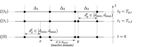
Figure 1: An example of the one-epoch coalescence process starting from $\xi(0)$. At time $t=0$, the domain of length $d$ is inactive since $d\geq d_{\max}$. At time $t_{1}$, site $x$ disappears and since $t_{1}=T_{x,\ell}$, the domain on the left of $x$ incorporates the domain on the right of $x$. Analogously at $t_{2}$ point $y$ disappears since the domain on the right of $y$ incorporates the domain on the left of $y$. The domain $\Delta_{1}$ and $\Delta_{3}$ are inactive since they are resulting from a coalescence. The domain $\Delta_{2}$ is frozen for $t>t_{2}$, due to the presence of $\Delta_{1}$ and $\Delta_{3}$. This illustrates the blocking effect.

We can now explain the dynamical meaning of assumptions (A1) and (A2):

• (A1) means that a domain is active, that is, it can incorporate another domain, iff its length $d$ lies in $[d_{\min},d_{\max})$.

• (A2) means that a domain resulting from a coalescence is not active.

As consequence, the following blocking effect appears: given three nearest-neighbor inactive domains $\Delta_{1},\Delta_{2},\Delta_{3}$, the intermediate domain $\Delta_{2}$ is frozen, in the sense that its extreme points cannot be erased; see Figure 1.

By definition of the one-epoch coalescence process, points can only be removed. Therefore, on any finite interval $I$, $\xi(t)\cap I$ converges as $t\to\infty$, and the following lemma follows at once.

Lemma 2.12

For any given initial condition $\xi\in{\mathcal{N}}(d_{\min})$ the following hold:

$\xi(t)\subset\xi(s)$ if $s\leq t$;

the configuration $\xi(t)$ is constant on bounded intervals eventually in $t$;

there exists a unique element $\xi(\infty)$ in ${\mathcal{N}}(d_{\max})$ such that $\xi(t)\cap I=\xi(\infty)\cap I$ for all large enough $t$ (depending on $I$) and all bounded intervals $I$.

Due to the above lemma, $\xi(\infty)$, the SPP representing the asymptotical state of the coalescence process, is well defined. Our first main result is given by the following two theorems. It states that, starting from a left-bounded renewal (resp., a $\mathbb{Z}$-stationary or stationary renewal) SPP $\xi$, at a later time $t$ the coalescence process $\xi(t)$ remains of the same type. Moreover, there exists a key identity between the Laplace transform of the interval law at time $t=0$ and time $t=\infty$. This equation, that we call one-epoch recursive equation, will play a crucial role in a recursive scheme for the hierarchical coalescence process.

Theorem 2.13 ((Renewal property))

Let $\nu,\mu$ be probability measures on ${\mathbb{R}}$ and $[d_{\min},\infty)$, respectively. Then, for all $t\in[0,\infty]$ there exist probability measures $\nu_{t},\mu_{t}$ on ${\mathbb{R}}$ and $[d_{\min},\infty)$, respectively, such that $\nu_{0}=\nu$, $\mu_{0}=\mu$ and:

if ${\mathcal{Q}}=\operatorname{Ren}(\nu,\mu)$, then ${\mathcal{Q}}_{t}=\operatorname{Ren}(\nu_{t},\mu_{t})$;

if ${\mathcal{Q}}=\operatorname{Ren}(\mu)$, then ${\mathcal{Q}}_{t}=\operatorname{Ren}(\mu_{t})$;

if ${\mathcal{Q}}=\operatorname{Ren}_{\mathbb{Z}}(\mu)$, then ${\mathcal{Q}}_{t}=\operatorname{Ren}_{\mathbb{Z}}(\mu_{t})$;

If ${\mathcal{Q}}=\operatorname{Ren}({\delta}_{0},\mu)$, then ${\mathcal{Q}}_{t}(\cdot\mid 0\in\xi)=\operatorname{Ren}({\delta}_{0},\mu_{t})$;

$\lim_{t\to\infty}\nu_{t}=\nu_{\infty}$ and $\lim_{t\to\infty}\mu_{t}=\mu_{\infty}$ weakly.

Theorem 2.14 ((Recursive identities))

Let $\nu,\mu$ be probability measures on ${\mathbb{R}}$ and $[d_{\min},\infty)$, respectively, and let $\nu_{t},\mu_{t}$ be the probability measures introduced in Theorem 2.13.

1. [(ii)]

2. Consider the Laplace/characteristic functions

   $$G_{t}(s) = \int_{[d_{\min},\infty)}e^{-sx}\mu_{t}(dx),\qquad s\in{\mathbb{R}}_{+}\cup i{\mathbb{R}},$$ (9)

   $$H_{t}(s) = \int_{[d_{\min},d_{\max})}e^{-sx}\mu_{t}(dx),\qquad s\in{\mathbb{R}}_{+}\cup i{\mathbb{R}}.$$ (10)

   Then, for any $s\in{\mathbb{R}}_{+}\cup i{\mathbb{R}}$, the following one-epoch recursive equation holds:

   $$1-G_{\infty}(s)=[1-G_{0}(s)]e^{H_{0}(s)}.$$ (11)

3. Consider the Laplace/characteristic function

   $$L_{t}(s)=\int e^{-sx}\nu_{t}(dx),\qquad s\in{\mathbb{R}}_{+}\cup\in i{\mathbb{R}}.$$

   1. [(b)]

   2. If ${\lambda}_{r}\equiv 0$, then $\nu_{t}=\nu_{0}$ for all $t\geq 0$. Hence $L_{t}(s)=L_{0}(s)$ for all $t\geq 0$.

   3. If ${\lambda}_{\ell}=\gamma{\lambda}_{r}$ for some $\gamma\in[0,\infty)$, then, for any $s\in{\mathbb{R}}_{+}\cup i{\mathbb{R}}$,

      $$L_{\infty}(s)=L_{0}(s)\exp\biggl{\{}\frac{H_{0}(s)-H_{0}(0)}{1+\gamma}\biggr{\}}.$$ (12)

      Moreover, if ${\mathcal{Q}}=\operatorname{Ren}(\nu,\mu)$

      $$\mathbb{P}_{\mathcal{Q}}\bigl{(}x_{0}(0)\in\xi(\infty)\bigr{)}=e^{-{H_{0}(0)}/({1+\gamma})},$$ (13)

      where $x_{0}(0)$ denotes the first point of the initial configuration $\xi(0)$.

The proofs of Theorems 2.13 and 2.14 are given in Sections 3 and 4.

Remark 2.15.

In (ii) we have analyzed two cases [(a) and (b)] motivated by the East model and by the Paste-all model. The arguments used in the proof of point (ii) could, however, be applied to other cases as well. We stress that the Laplace transform $L_{t}(s)$, $s\in{\mathbb{R}}_{+}$, could diverge since $\nu_{t}$ has support on ${\mathbb{R}}$. Therefore, the above identities in point (ii) have to be thought of as identities in the extended space $[0,\infty]$.

We point out that the one-epoch recursive equation (11) uniquely determines $\mu_{\infty}$ when knowing $\mu_{0},d_{\min},d_{\max}$. In particular, these three elements are the unique traces of the dynamics that asymptotically survive. In other words, the precise form of the rates ${\lambda}_{\ell}$ and ${\lambda}_{r}$ is irrelevant. In the case of a left-bounded renewal point process the limiting first point law $\nu_{\infty}$ does not share such a universality, although the trace of ${\lambda}_{\ell}$ and ${\lambda}_{r}$ on $\nu_{\infty}$ is only partial.

Remark 2.16.

Assume for simplicity that $\mu$ is concentrated on ${\mathbb{N}}_{+}$, so that the domains have integer length at any time. After properly constructing the Markov generator (8) one could prove that

$$\qquad\partial_{t}\mu_{t}(d)=-{\lambda}(d)\mu_{t}(d)+\sum_{x=1}^{d-1}[{\lambda}_{\ell}(x)+{\lambda}_{r}(d-x)]\mu_{t}(x)\mu_{t}(d-x).$$ (14)

Note that if $d$ is active, then only the first addendum in the right-hand side is present, while if $d$ is inactive this first addendum is absent. From this observation, one easily obtains that $\partial_{t}G_{t}=(1-G_{t})\partial_{t}H_{t}$, and therefore

$$1-G_{t}(s)=\bigl{(}1-G_{0}(s)\bigr{)}\exp\{H_{0}(s)-H_{t}(s)\}\qquad\forall t,s\geq 0.$$ (15)

Taking the limit $t\to\infty$ one gets (11). This strategy has been applied in SE , where the treatment is not rigorous, and will be formalized in FMRT2 in order to treat other coalescence processes as in BDG . It could be applied to derive (12). While the Smoluchoswski-type equation (14) has a mean-field structure (see, e.g., A ), in proving (11) and (12), we have followed here a more constructive strategy, and we have investigated how a domain of given length can emerge at the end of the epoch or how a given point can become the first point for the configuration $\xi(\infty)$ at the end of the epoch.

2.3 The hierarchical coalescence process

We can finally introduce the hierarchical coalescence process (HCP). The dynamics depend on the following parameters and functions: a strictly increasing sequence of positive numbers $\{d^{(n)}\}_{n\geq 1}$ and a family of uniformly bounded functions ${\lambda}_{\ell}^{(n)},{\lambda}_{r}^{(n)}\dvtx[d^{(n)},\allowbreak\infty]\rightarrow[0,A],n\geq 1$. Without loss of generality we may assume that $d^{(1)}=1$. We set as before ${\lambda}^{(n)}:={\lambda}^{(n)}_{\ell}+{\lambda}^{(n)}_{r}$, and we assume: [(A3)]

for any $n\in{\mathbb{N}}_{+}$, ${\lambda}^{(n)}(d)>0$ if and only if $d\in[d^{(n)},d^{(n+1)})$;

for any $n\in{\mathbb{N}}_{+}$, if $d,d^{\prime}\geq d^{(n)}$, then $d+d^{\prime}\geq d^{(n+1)}$ (i.e., $2d^{(n)}\geq d^{(n+1)}$);

$\lim_{n\to\infty}d^{(n)}=\infty$. For example, one could take $d^{(n)}=n$ or $d^{(n)}=a^{n-1}$ with $a\in(1,2]$.

The HCP is then given by a sequence of one-epoch coalescence processes, suitably linked. More precisely, the stochastic evolution of the HCP is described by the sequence of paths $\{\xi^{(n)}(\cdot)\}_{n\geq 1}$ where each $\xi^{(n)}$ is the random path describing the evolution of the one-epoch coalescence process with rates ${\lambda}^{(n)}_{\ell},{\lambda}^{(n)}_{r}$, active domain lengths $d^{(n)}_{\min}=d^{(n)},d^{(n)}_{\max}=d^{(n+1)}$ and initial condition $\xi^{(n)}(0)=\xi^{(n-1)}(\infty)$, $n\geq 2$. Informally we refer to $\xi^{(n)}$ as describing the evolution in the $n$th epoch. See Figure 2 for a graphical illustration.

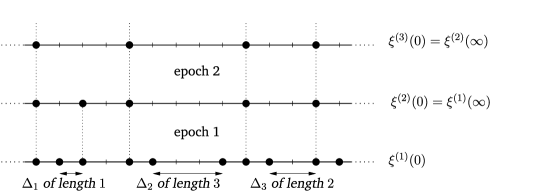
Figure 2: An example of HCP dynamics, with $d^{(n)}=n$. The distances between the points are, from left to right, $1$, $1$ (corresponding to $\Delta_{1}$), $2$, $1$, $3$ (corresponding to $\Delta_{2}$), $1$, $1$, $2$ (corresponding to $\Delta_{3}$)$\ldots.$ At the beginning of epoch 1, only the domains of length in $1$ are active. In particular, $\Delta_{1}$ is active while $\Delta_{2}$ and $\Delta_{3}$ are inactive. At the end of epoch 1, there are no more domains of length less than $2$ (see Lemma 2.12). At the beginning of epoch 2, domains of length $2$ are active and at the end, there are no more domains of length less than $3$, and so on. Note that an inactive domain as $\Delta_{2}$ can increase its length.

Theorem 2.13 gives us information on the evolution and its asymptotic inside each epoch when the initial condition is a SPP of the renewal type. If, for example, the initial distribution ${\mathcal{Q}}$ for the first epoch is $\operatorname{Ren}(\nu,\mu)$, we can use Theorem 2.13 together with the link $\xi^{(n+1)}(0)=\xi^{(n)}(\infty)$ between two consecutive epochs to recursively define the measures $\mu^{(n)},\nu^{(n)}$ by

$$\mu^{(n+1)} = \mu_{\infty}^{(n)},\qquad\mu^{(1)}=\mu,$$

$$\nu^{(n+1)} = \nu_{\infty}^{(n)},\qquad\nu^{(1)}=\nu.$$

With this position it is then natural to ask if, in some suitable sense, the measures $\mu^{(n)},\nu^{(n)}$ have a well-defined limiting behavior as $n\to\infty$. The affirmative answer is contained in the following theorem, which is the core of the paper. Before stating it we need a result on the Laplace transform of probability measures on $[1,\infty]$.

Lemma 2.17

Let $\mu$ be a probability measure on $[1,\infty)$, and let $g(s)$ be its Laplace transform, that is, $g(s)=\int e^{-sx}\mu(dx),s>0$.

1. [(ii)]

2. If

   $$\lim_{s\downarrow 0}-\frac{sg^{\prime}(s)}{1-g(s)}=c_{0},$$ (17)

   then necessarily $0\leq c_{0}\leq 1$.

3. The existence of limit (17) holds if:

   1. [(a)]

   2. $\mu$ has finite mean and then $c_{0}=1$, or

   3. for some ${\alpha}\in(0,1)$ $\mu$ belongs to the domain of attraction of an ${\alpha}$-stable law or, more generally, $\mu((x,\infty))=x^{-{\alpha}}L(x)$ where $L(x)$ is a slowly varying function at $+\infty$, ${\alpha}\in[0,1]$, and in this case $c_{0}=\alpha$.

Remark 2.18.

One could wonder if limit (17) always exists. The answer is negative and an example is given in Appendix B.

The proof of Lemma 2.17 is discussed in Appendix A.

Theorem 2.19

Let $\nu,\mu$ be probability measures on ${\mathbb{R}}$ and $[1,\infty)$, respectively, and let $g(s)$ be the Laplace transform of $\mu$. Let ${\mathcal{Q}}$ be the initial law of $\xi^{(1)}$, and suppose that ${\mathcal{Q}}$ is either ${\mathcal{Q}}=\operatorname{Ren}(\nu,\mu)$ or ${\mathcal{Q}}=\operatorname{Ren}(\mu)$ or ${\mathcal{Q}}=\operatorname{Ren}_{\mathbb{Z}}(\mu)$. For any $n\in{\mathbb{N}}_{+}$ let $X^{(n)}$ be a random variable with law $\mu^{(n)}$ defined in (2.3) so that $g(s):={\mathbb{E}}[e^{-sX^{(1)}}]$.

If (17) holds for $g$, then the rescaled variable $Z^{(n)}:=X^{(n)}/d^{(n)}$ weakly converges to the random variable $Z^{(\infty)}\equiv Z^{(\infty)}_{c_{0}}$ whose Laplace transform is given by

$$g^{(\infty)}_{c_{0}}(s)=1-\exp\biggl{\{}-c_{0}\int_{1}^{\infty}\frac{e^{-sx}}{x}\,dx\biggr{\}}.$$ (18)

The corresponding probability density is of the form $z_{c_{0}}(x)\mathbh{1}_{x\geq 1}$, where $z_{c_{0}}$ is the continuous function on $[1,\infty)$ given by

$$z_{c_{0}}(x)=\sum_{k=1}^{\infty}\frac{(-1)^{k+1}c_{0}^{k}}{k!}\rho_{k}(x)\mathbh{1}_{x\geq k},$$ (19)

where $\rho_{1}(x)=1/x$ and

$$\rho_{k+1}(x)=\int_{1}^{\infty}dx_{1}\cdots\int_{1}^{\infty}dx_{k}\frac{1}{x-\sum_{i=1}^{k}x_{i}}\prod_{j=1}^{k}\frac{1}{x_{j}}\mathbh{1}_{\sum_{i=1}^{k}x_{i}\leq x-1},\qquad k\geq 1.$$

The proof of Theorem 2.19 is discussed in Section 6.2.

Remark 2.20.

The remarkable fact of the above result is that the only reminiscence of the initial distribution in the limiting law is through the constant $c_{0}$ which, as proved in Lemma 17, is “universal” for a large class of initial laws $\mu$. Hence the term universality in the title. We also stress that, starting with a stationary or ${\mathbb{Z}}$-stationary renewal SPP, the weak limit of $Z^{(n)}$ always exists and it is universal ($c_{0}=1$), not depending on the rates ${\lambda}^{(n)}_{\ell}$, ${\lambda}^{(n)}_{r}$.

Remark 2.21.

We point out that the asymptotic Laplace distribution $g^{(\infty)}_{c_{0}}$ can be written also as

$$g^{(\infty)}_{c_{0}}(s)=1-\exp\biggl{\{}-c_{0}\int_{s}^{\infty}\frac{e^{-x}}{x}\,dx\biggr{\}}=1-\exp\{-c_{0}\operatorname{Ei}(s)\},$$

where $\operatorname{Ei}(\cdot)$ denotes the exponential integral function. This is indeed the form appearing in DGY2 and SE with $c_{0}=1$ (see previous remark).

If the law $\mu$ has finite mean then by the above Theorem combined with (ii) of Lemma 2.17 we know that $Z^{(n)}$ weakly converges to the random variable $Z_{1}^{(\infty)}$. Actually we can improve our result to higher moments.

Proposition 2.22

In the same setting of Theorem 2.19 assume that $d^{(n)}=a^{n-1}$ for some $a\in(1,2]$, and that $\mu$ has finite $k$th moment, $k\in{\mathbb{N}}_{+}$. Then, for any function $f\dvtx[0,\infty)\to{\mathbb{R}}$ such that $|f(x)|\leq C+Cx^{k}$ for some constant $C$, it holds

$$\lim_{n\to\infty}{\mathbb{E}}\bigl{[}f\bigl{(}Z^{(n)}\bigr{)}\bigr{]}={\mathbb{E}}\bigl{[}f\bigl{(}Z_{1}^{(\infty)}\bigr{)}\bigr{]}.$$ (20)

Remark 2.23.

The choice $d^{(n)}=a^{n-1}$ in Proposition 2.22 is technical and could be relaxed, but at the price of extra hypotheses (that would not include the case $d^{(n)}=n$, e.g.). In order to keep the computations as simple as possible we decided to focus on this particular example which is of interest for applications to the East model.

The proof of Proposition 2.22 can be found in Section 6.5. Next we concentrate on the asymptotic behavior of the first point law when starting with a left-bounded renewal SPP.

Theorem 2.24

Let $\nu,\mu$ be probability measures on ${\mathbb{R}}$ and $[1,\infty)$, respectively, and consider the hierarchical coalescence process such that the initial law ${\mathcal{Q}}$ of $\xi^{(1)}$ is $\operatorname{Ren}(\nu,\mu)$. Assume

$${\lambda}^{(n)}_{\ell}=\gamma{\lambda}^{(n)}_{r}\qquad\forall n\geq 1,$$ (21)

for some $\gamma\in[0,\infty)$, and let, for any $n\in{\mathbb{N}}_{+}$, $X_{0}^{(n)}$ be the position of the first point of the HCP at the beginning of the $n$th epoch.

If limit (17) exists for the Laplace transform $g$ of $\mu$ then, as $n\to\infty$, the rescaled random variable $Y^{(n)}:=X_{0}^{(n)}/d^{(n)}$ weakly converges to the positive random variable $Y^{(\infty)}_{c_{0}}$ with Laplace transform given by

$${\mathbb{E}}\bigl{(}e^{-sY^{(\infty)}_{c_{0}}}\bigr{)}=\exp\biggl{\{}-\frac{c_{0}}{1+\gamma}\int_{(0,1)}\frac{1-e^{-sy}}{y}\,dy\biggr{\}},\qquad s\in{\mathbb{R}}_{+}.$$ (22)

We point out that if ${\lambda}_{r}^{(n)}\equiv 0$ for all $n\geq 1$, the first point does not move. In particular, its asymptotic is trivial. Theorem 2.24 is proven in Section 6.3.

Finally, we evaluate the surviving probability of a given point:

Theorem 2.25

Let $\nu,\mu$ be probability measures on ${\mathbb{R}}$ and $[1,\infty)$, respectively, and consider the hierarchical coalescence process with initial law ${\mathcal{Q}}$. Assume

$${\lambda}^{(n)}_{\ell}=\gamma{\lambda}^{(n)}_{r}\qquad\forall n\geq 1,$$ (23)

for some $\gamma\in[0,\infty)$, and let, for any $n\in{\mathbb{N}}_{+}$, $X_{0}^{(n)}$ be the position of the first point of the HCP at the beginning of the $n$th epoch.

If the limit (17) exists for the Laplace transform $g$ of $\mu$ then, as $n\to\infty$:

if ${\mathcal{Q}}=\operatorname{Ren}(\nu,\mu)$, then:

$$\mathbb{P}_{{\mathcal{Q}}}\bigl{(}X_{0}^{(n)}=X_{0}^{(1)}\bigr{)}=\bigl{(}1/d^{(n)}\bigr{)}^{({c_{0}}/({1+\gamma}))(1+o(1))};$$

if ${\mathcal{Q}}=\operatorname{Ren}(\mu\mid 0)$, then

$$\mathbb{P}_{{\mathcal{Q}}}\bigl{(}0\in\xi^{(n)}(0)\bigr{)}=\bigl{(}1/d^{(n)}\bigr{)}^{c_{0}(1+o(1))}.$$

Note that (ii) does not depend on the value of $\gamma$. Theorem 2.25 is proven in Section 6.4.

Extension of the above results to one-epoch coalescence process or hierarchical coalescence process with initial law ${\mathcal{Q}}$ describing an exchangeable SPP will be discussed in Appendix D.

3 Renewal property in the OCP: Proof of Theorem 2.13

In this section and in the next one we will prove our results concerning the one-epoch coalescence process (Theorems 2.13 and 2.14) in a more general setting, namely when the interval $[d_{\min},d_{\max})$ is replaced by a more general set ${\mathcal{A}}\subset(0,\infty)$. More precisely, let ${\lambda}_{\ell},{\lambda}_{r}$ be bounded nonnegative functions on $(0,\infty]$, and set ${\lambda}={\lambda}_{\ell}+{\lambda}_{r}$. We assume that: [(A2^′)]

${\lambda}(d)>0$ if and only if $d\in{\mathcal{A}}$;

if $d,d^{\prime}\geq\inf({\mathcal{A}})$, then $d+d^{\prime}\notin{\mathcal{A}}$. Above, $d_{\min}:=\inf({\mathcal{A}})$ denotes the infimum of the set ${\mathcal{A}}$. When ${\mathcal{A}}=[d_{\min},\allowbreak d_{\max})$, (A1^′) and (A2^′) coincide with assumptions (A1) and (A2), respectively. A domain is called active if its length belongs to ${\mathcal{A}}$. The initial distribution ${\mathcal{Q}}$ of the one-epoch coalescence must be supported in $[\inf({\mathcal{A}}),\infty)$. In (9) and (10) the integration domains become $[\inf({\mathcal{A}}),\infty)$ and ${\mathcal{A}}$, respectively.

The proof of Theorem 2.13 requires the definition of a universal coupling, that is, the construction on the same probability space of all one-epoch coalescence processes obtained by varying the initial configuration. This coupling will be relevant also in the proof of Theorem 2.25(ii).

3.1 Universal coupling for the domain dynamics

In Section 2 we have introduced some enumerations of the points in $\xi\in{\mathcal{N}}$, depending on the property of $\xi$ to be unbounded both from the left and from the right, or only from the left. It is convenient here to have a universal enumeration. To this aim, given $\xi\in{\mathcal{N}}$, we enumerate its points in increasing order, with the rule that the smallest positive one (if it exists) gets the label $1$, while the largest nonpositive one (if it exists) gets the label $0$. We write $N(x,\xi)$ for the integer number labeling the point $x\in\xi$. This allows to enumerate the domains of $\xi$ as follows: a domain $[x,x^{\prime}]$ is said to be the $k$th domain if (i) $x$ is finite and $N(x,\xi)=k$, or (ii) $x=-\infty$ and $N(x^{\prime},\xi)=k+1$. Recall that if $x=-\infty$, then $\xi$ is unbounded from the left and $x^{\prime}$ is the smallest number in $\xi$.

We set $\|{\lambda}\|_{\infty}=\sup_{d\in\mathcal{A}}{\lambda}(d)$, and we define ${\lambda}^{*}_{\ell}={\lambda}_{r},{\lambda}^{*}_{r}={\lambda}_{\ell}$. Obviously ${\lambda}={\lambda}_{\ell}+{\lambda}_{r}={\lambda}_{\ell}^{*}+{\lambda}_{r}^{*}$. This change of notation should help the reader. Indeed, in the point dynamics a point $x$ is erased by the action of its left (right) domain of length $d$ with rate ${\lambda}_{\ell}(d)$ (${\lambda}_{r}(d)$). On the other hand, as explained again below, if we formulate the model in terms of a domain dynamics then a domain of length $d$ disappears because of the annihilation of its left (right) extreme with probability rate ${\lambda}_{\ell}^{*}(d)$ (${\lambda}_{r}^{*}(d)$).

We consider now a probability space $({\Omega},{\mathcal{F}},P)$ on which the following random objects are defined and are all independent: the Poisson processes ${\mathcal{T}}^{(k)}=\{T_{m}^{(k)}\dvtx m\in{\mathbb{N}}\}$ and $\bar{\mathcal{T}}^{(k)}=\{\bar{T}_{m}^{(k)}\dvtx m\in{\mathbb{N}}\}$ of parameter $\|{\lambda}\|_{\infty}$, indexed by $k\in{\mathbb{Z}}$, and the random variables $U^{(k)}_{m}$, $\bar{U}^{(k)}_{m}$, uniformly distributed in $[0,1]$, indexed by $k\in{\mathbb{Z}}$ and $m\in{\mathbb{N}}$.

Next, given $\zeta\in{\mathcal{N}}(d_{\min})$ and ${\omega}\in{\Omega}$, to each domain $\Delta$ that belongs to $\zeta$ we associate the Poisson process ${\mathcal{T}}^{(k)}$ if $\Delta$ is the $k$th domain in $\zeta$. In this case, we write ${\mathcal{T}}^{(\Delta)}$ instead of ${\mathcal{T}}^{(k)}$. Similarly we define $\bar{\mathcal{T}}^{(\Delta)}$, $U^{(\Delta)}_{m}$, $\bar{U}^{(\Delta)}_{m}$. We define ${\mathcal{W}}_{t}[{\omega},\zeta]$ as the set of domains $\Delta$ in $\zeta$ such that

$$\bigl{\{}s\in[0,t]\dvtx s\in{\mathcal{T}}^{(\Delta)}\cup\bar{\mathcal{T}}^{(\Delta)},\mbox{ or }s\in{\mathcal{T}}^{(\Delta^{\prime})}\cup\bar{\mathcal{T}}^{(\Delta^{\prime})}$$

$$\hskip 61.7pt\mbox{for some domain }\Delta^{\prime}\mbox{ neighboring }\Delta\bigr{\}}\not=\varnothing.$$

On ${\mathcal{W}}_{t}[{\omega},\zeta]$ we define a graph structure putting an edge between domains $\Delta$ and $\Delta^{\prime}$ if and only if they are neighboring in $\zeta$. Since the function ${\lambda}$ is bounded from above, we deduce that the set

$${\mathcal{B}}(\zeta)\!:=\!\{{\omega}\dvtx{\mathcal{W}}_{t}[{\omega},\zeta]\mbox{ has all connected components of finite cardinality }\forall t\!\geq\!0\}$$

has $P$-probability equal to $1$. Note that the event ${\mathcal{B}}(\zeta)$ depends on $\zeta$ only through the infimum and the supremum of the set $\{N(x,\zeta)\in{\mathbb{Z}}\dvtx x\in\zeta\}$. By a simple argument based on countability, we conclude that $P({\mathcal{B}})=1$, where ${\mathcal{B}}$ is defined as the family of elements ${\omega}\in{\Omega}$ belonging to $\bigcap_{\zeta\in{\mathcal{N}}(d_{\min})}{\mathcal{B}}(\zeta)$ and such that all the sets ${\mathcal{T}}^{(k)}[{\omega}]$ and $\bar{\mathcal{T}}^{(k)}[{\omega}]$, $k\in{\mathbb{Z}}$, are disjoint.

In order to define the path $\{\xi(s)\}_{s\geq 0}\equiv\{\xi^{\zeta}(s,{\omega})\}_{s\geq 0}$ we first fix a time $t>0$ and define the path up to time $t$. If ${\omega}\notin{\mathcal{B}}$, then we set

$$\xi(s)=\zeta\qquad\forall s\in[0,t].$$

If ${\omega}\in{\mathcal{B}}$, recall the definition of the graph ${\mathcal{W}}_{t}[{\omega},\zeta]$. Given a set of domains $V$ we write $\bar{V}$ for the set of the associated extremes, that is, $x\in\bar{V}$ if and only if there exists a domain in $V$ having $x$ as left or right extreme. Moreover, we write ${\mathcal{V}}_{t}[{\omega},\zeta]$ for the set of all domains in $\zeta$ that do not belong to ${\mathcal{W}}_{t}[{\omega},\zeta]$. We define

$$\xi(s)\cap\overline{{\mathcal{V}}_{t}[{\omega},\zeta]}:=\overline{{\mathcal{V}}_{t}[{\omega},\zeta]}\qquad\forall s\in[0,t],$$ (24)

that is, up to time $t$ all points in $\overline{{\mathcal{V}}_{t}[{\omega},\zeta]}$ survive. Let us now fix a cluster ${\mathcal{C}}$ in the graph ${\mathcal{W}}_{t}[{\omega},\zeta]$. The path $(\xi(s)\cap\bar{\mathcal{C}}\dvtx s\in[0,t])$ is implicitly defined by the following rules (the definition is well posed since ${\omega}\in{\mathcal{B}}$). If $s\in[0,t]$ equals $T^{(\Delta)}_{m}$ with $\Delta=[x,x^{\prime}]\in{\mathcal{C}}$ and $x,x^{\prime}\in\xi(s-)$, then the ring at time $T^{(\Delta)}_{m}$ is called legal if

$$U_{m}^{(\Delta)}\leq\frac{{\lambda}_{\ell}^{*}(x^{\prime}-x)}{\|{\lambda}\|_{\infty}},$$ (25)

and in this case we set $\xi(s)\cap\bar{\mathcal{C}}:=(\xi(s-)\cap\bar{\mathcal{C}})\setminus\{x\}$, otherwise we set $\xi(s)\cap\bar{\mathcal{C}}=\xi(s-)\cap\bar{\mathcal{C}}$. In the first case, we say that $x$ is erased and that the domain $[x,x^{\prime}]$ has incorporated the domain on its left. Similarly, if $s\in[0,t]$ equals $\bar{T}^{(\Delta)}_{m}$ with $\Delta=[x,x^{\prime}]\in{\mathcal{C}}$ and $x,x^{\prime}\in\xi(s-)$, then the ring at time $\bar{T}^{(\Delta)}_{m}$ is called legal if

$$\bar{U}_{m}^{(\Delta)}\leq\frac{{\lambda}_{r}^{*}(x^{\prime}-x)}{\|{\lambda}\|_{\infty}},$$ (26)

and in this case we set $\xi(s)\cap\bar{\mathcal{C}}:=(\xi(s-)\cap\bar{\mathcal{C}})\setminus\{x^{\prime}\}$, otherwise we set $\xi(s)\cap\bar{\mathcal{C}}=\xi(s-)\cap\bar{\mathcal{C}}$. Again, in the first case we say that $x^{\prime}$ is erased and that the domain $[x,x^{\prime}]$ has incorporated the domain on its right.

We point out that $\bar{\mathcal{C}}\cap\bar{\mathcal{C}}^{\prime}=\varnothing$ if ${\mathcal{C}}$ and ${\mathcal{C}}^{\prime}$ are distinct clusters in ${\mathcal{W}}_{t}[{\omega},\zeta]$. On the other hand, it could be $\bar{\mathcal{C}}\cap\overline{{\mathcal{V}}_{t}[{\omega},\zeta]}\not=\varnothing$. Let $x$ be a point in the intersection, and suppose for example that $[a,x]\in{\mathcal{C}}$ while $[x,b]\in{\mathcal{V}}_{t}[{\omega},\zeta]$. Then, by definition of ${\mathcal{W}}_{t}[{\omega},\zeta]$, one easily derives that the Poisson processes associated to the domains $[a,x]$ and $[x,b]$ do not intersect $[0,t]$, while at least one of the Poisson processes associated to the domain on the left of $[a,x]$ intersects $[0,t]$. In particular, $x\in\xi(s)\cap\bar{\mathcal{C}}$ for all $s\in[0,t]$, in agreement with (24). The same conclusion is reached if $[a,x]\in{\mathcal{V}}_{t}[{\omega},\zeta]$ and $[x,b]\in{\mathcal{C}}$. This allows to conclude that the definition of the path $\{\xi(s)\}_{s\geq 0}$ up to time $t$ is well posed. We point out that this definition is $t$-dependent. The reader can easily check that, increasing $t$, the resulting paths coincide on the intersection of their time domains. Joining these paths together we get $\{\xi(s)\}_{s\geq 0}$.

At this point, it is simple to check that, given a configuration $\zeta\in{\mathcal{N}}(d_{\min})$, the law of the corresponding path $\{\xi(s)\}_{s\geq 0}$ is that of the one-epoch coalescence process defined in Section 2 with initial condition $\zeta$. The advantage of the above construction is that all one-epoch coalescence processes, obtained by varying the initial configuration, can be realized on the the same probability space. Given a probability measure ${\mathcal{Q}}$ on ${\mathcal{N}}(d_{\min})$, the one-epoch coalescence process with initial distribution ${\mathcal{Q}}$ can be realized by the random path $\{\xi^{\cdot}(s,\cdot)\}_{s\geq 0}$, defined on the product space ${\Omega}\times{\mathcal{N}}(d_{\min})$, endowed with the probability measure $P\times{\mathcal{Q}}$.

3.2 Proof of Theorem 2.13(i)–(iii)

Before presenting the proof of Theorem 2.13(i)–(iii) we state and prove a key lemma.

Lemma 3.1 ((Separation effect))

For any $x\in{\mathbb{R}}$, any configuration $\zeta\in{\mathcal{N}}(d_{\min})$ with $x\in\zeta$, any event $\mathcal{A}$ in the $\sigma$-algebra generated by $\{\xi(s)\cap(-\infty,x)\}_{s\leq t}$, any event $\mathcal{B}$ in the $\sigma$-algebra generated by $\{\xi(s)\cap(x,\infty)\}_{s\leq t}$, it holds

$${\mathbb{P}}_{\zeta}\bigl{(}\mathcal{A}\cap{\mathcal{B}}\cap\{x\in\xi(t)\}\bigr{)}$$

(27)

$$\qquad={\mathbb{P}}_{\zeta\cap(-\infty,x]}\bigl{(}{\mathcal{A}}\cap\{x\in\xi(t)\}\bigr{)}{\mathbb{P}}_{\zeta\cap[x,\infty)}\bigl{(}{\mathcal{B}}\cap\{x\in\xi(t)\}\bigr{)}.$$

We set $\zeta_{\ell}:=\zeta\cap(-\infty,x]$, $\zeta_{r}:=\zeta\cap[x,\infty)$, $k:={\mathcal{N}}(x,\zeta)$, $j:=\mathcal{N}(x,\zeta_{\ell})$ and $u:=\mathcal{N}(x,\zeta_{r})$. The desired result (3.1) is implied by the following facts (i) and (ii):

For any $\omega\in{\Omega}$ such $x\in\xi^{\zeta}(t,\omega)$ the following holds. At each time $s\in[0,t]$ one has

$$\xi^{\zeta_{\ell}}(s,\hat{\omega})=\xi^{\zeta}(s,\omega)\cap(-\infty,x],$$

if $\hat{\omega}$ satisfies for any $i<k$ and $m\in{\mathbb{N}}$

$${\mathcal{T}}^{(i)}({\omega})={\mathcal{T}}^{(i+j-k)}(\hat{\omega}),\qquad U_{m}^{(i+j-k)}({\omega})=U_{m}^{(i+j-k)}(\hat{\omega}),$$ (28)

and the same identities with ${\mathcal{T}}$ and $U_{m}^{(\cdot)}$ replaced by $\bar{\mathcal{T}}$ and $\bar{U}_{m}^{(\cdot)}$. Similarly, at each time $s\in[0,t]$ one has

$$\xi^{\zeta_{r}}(s,\tilde{\omega})=\xi^{\zeta}(s,\omega)\cap[x,\infty),$$

if $\tilde{\omega}$ satisfies for any $i\geq k$ and $m\in{\mathbb{N}}$

$${\mathcal{T}}^{(i)}({\omega})={\mathcal{T}}^{(i+u-k)}(\tilde{\omega}),\qquad U_{m}^{(i)}({\omega})=U_{m}^{(i+u-k)}(\tilde{\omega}),$$ (29)

and the same identities with ${\mathcal{T}}$ and $U^{(\cdot)}_{m}$ replaced by $\bar{\mathcal{T}}$ and $\bar{U}^{(\cdot)}_{m}$.

Take $\hat{\omega},\tilde{\omega}\in{\Omega}$ such that $x\in\xi^{\zeta_{\ell}}(t,\hat{\omega})$ and $x\in\xi^{\zeta_{r}}(t,\tilde{\omega})$. At each time $s\in[0,t]$ it holds

$$\xi^{\zeta}(s,\omega)=\xi^{\zeta_{\ell}}(s,\hat{\omega})\cup\xi^{\zeta_{r}}(s,\tilde{\omega}),$$

if ${\omega}\in{\Omega}$ satisfies (28) and the same identities with ${\mathcal{T}}$ and $U^{(\cdot)}_{m}$ replaced by $\bar{\mathcal{T}}$ and $\bar{U}^{(\cdot)}$ for any $i<k$ and $m\in{\mathbb{N}}$, and ${\omega}$ satisfies (29) and the same identities with ${\mathcal{T}}$ and $U^{(\cdot)}_{m}$ replaced by $\bar{\mathcal{T}}$ and $\bar{U}^{(\cdot)}_{m}$ for any $i\geq k$ and $m\in{\mathbb{N}}$. ∎

We first prove the renewal property for the OCP with initial distribution ${\mathcal{Q}}=\operatorname{Ren}(\nu,\mu)$. We take the special realization of the process defined by means of the universal coupling at the end of the previous section. We concentrate on the joint distribution of the random variables $x_{0}(t),d_{1}(t),d_{2}(t)$, proving that they are independent and giving an expression of their marginal distributions. We recall that $x_{0}(t)$ is the leftmost point of $\xi(t)$, while $d_{k}(t)$ is the length of the $k$th domain to the right of $x_{0}(t)$ in $\xi(t)$.

While $d_{1}(t),d_{2}(t)$ are nonnegative random variables and their Laplace transforms are always finite, $x_{0}(t)$ is a real random variable and its Laplace transform could diverge. Hence, it is convenient to work with characteristic functions instead of Laplace transforms. Given imaginary numbers $s_{0},s_{1},s_{2}\in i{\mathbb{R}}$, we have

$${\mathbb{E}}_{{\mathcal{Q}}}\bigl{(}e^{-s_{0}x_{0}(t)-s_{1}d_{1}(t)-s_{2}d_{2}(t)}\bigr{)}$$

$$\qquad=\sum_{i_{0}<i_{1}<i_{2}\in{\mathbb{N}}}{\mathbb{E}}_{{\mathcal{Q}}}\bigl{(}e^{-s_{0}x_{0}(t)-s_{1}d_{1}(t)-s_{2}d_{2}(t)};x_{0}(t)=x_{i_{0}}(0);$$

(30)

$$\hskip 137.0ptx_{1}(t)=x_{i_{1}}(0);x_{2}(t)=x_{i_{2}}(0)\bigr{)}$$

$$\qquad=\sum_{i_{0}<i_{1}<i_{2}\in{\mathbb{N}}}\int{\mathcal{Q}}(d\zeta)e^{-s_{0}x_{i_{0}}-s_{1}(x_{i_{1}}-x_{i_{0}})-s_{2}(x_{i_{2}}-x_{i_{1}})}f_{i_{0},i_{1},i_{2}}(\zeta),$$

where $\zeta=\{x_{k}\dvtx k\in{\mathbb{N}}\}$ and the function $f_{i_{0},i_{1},i_{2}}(\zeta)$ is defined as the $P$-probability of the event ${\mathcal{U}}$ in ${\Omega}$ given by the elements ${\omega}$ satisfying the following properties:

$$\mbox{(P1)}\quad\xi^{\zeta}(t,{\omega})\cap(-\infty,x_{i_{0}}] = \{x_{i_{0}}\},$$

$$\mbox{(P2)}\quad\xi^{\zeta}(t,{\omega})\cap[x_{i_{0}},x_{i_{1}}] = \{x_{i_{0}},x_{i_{1}}\},$$

$$\mbox{(P3)}\quad\xi^{\zeta}(t,{\omega})\cap[x_{i_{1}},x_{i_{2}}] = \{x_{i_{1}},x_{i_{2}}\}.$$

Let us now set

$$\zeta_{0} = \zeta\cap(-\infty,x_{i_{0}}],\qquad\zeta_{0,1}=\zeta\cap[x_{i_{0}},x_{i_{1}}],$$

$$\zeta_{1,2} = \zeta\cap[x_{i_{1}},x_{i_{2}}],\qquad\zeta_{2}=\zeta\cap[x_{i_{2}},\infty).$$

Then, by the separation effect described in Lemma 3.1, one has

$$f_{i_{0},i_{1},i_{2}}(\zeta)=P({\mathcal{U}}(\zeta))=\prod_{i=1}^{4}P\bigl{(}{\omega}\in{\Omega}\dvtx{\omega}\mbox{ fulfills }\mbox{(P$i^{\prime}$)}\bigr{)},$$ (31)

where

$$\mbox{(P1${}^{\prime}$)}\quad\hskip 5.9pt\xi^{\zeta_{0}}(t,{\omega})=\{x_{i_{0}}\},$$

$$\mbox{(P2${}^{\prime}$)}\quad\xi^{\zeta_{0,1}}(t,{\omega})=\{x_{i_{0}},x_{i_{1}}\},$$

$$\mbox{(P3${}^{\prime}$)}\quad\xi^{\zeta_{1,2}}(t,{\omega})=\{x_{i_{1}},x_{i_{2}}\},$$

$$\mbox{(P4${}^{\prime}$)}\quad\hskip 32.0ptx_{i_{2}}\in\xi^{\zeta_{2}}(t,{\omega}).$$

We stress that the factors in (31) are $\zeta$-dependent, although we have omitted $\zeta$ from the notation. In particular, the probability $P({\omega}\in{\Omega}\dvtx{\omega}\mbox{ fulfills }\mbox{(P$i^{\prime}$)})$ depends on $\zeta$ only through the first point $x_{0}$ and the domain lengths $d_{1},d_{2},\ldots,\allowbreak d_{i_{0}}$ if $i=1$, the domain lengths $d_{i_{0}+1},\ldots,d_{i_{1}}$ if $i=2$, the domain lengths $d_{i_{1}+1},\ldots,d_{i_{2}}$ if $i=3$ and the domain lengths $d_{i_{2}+1},d_{i_{2}+2},\ldots$ if $i=4$. Thinking of $\zeta$ as a random configuration sampled by ${\mathcal{Q}}$, all the above domain lengths are i.i.d. with law $\mu$ and are independent from $x_{0}$ which has law $\nu$. In particular, the random variables $\zeta\to P({\omega}\in{\Omega}\dvtx{\omega}\mbox{ fulfills (P$i^{\prime}$)})$ are independent for $i=1,\ldots,4$. Using the consequent factorization and integrating over $\zeta$ in (3.2), we conclude that

$${\mathbb{E}}_{{\mathcal{Q}}}\bigl{(}e^{-s_{0}x_{0}(t)-s_{1}d_{1}(t)-s_{2}d_{2}(t)}\bigr{)}$$

$$\qquad=\sum_{i_{0}<i_{1}<i_{2}\in{\mathbb{N}}}\int{\mathcal{Q}}(d\zeta)P\bigl{(}{\omega}\in{\Omega}\dvtx{\omega}\mbox{ fulfills (P4${}^{\prime}$)}\bigr{)}$$

$$\hskip 41.6pt\qquad\quad{}\times\int{\mathcal{Q}}(d\zeta)e^{-s_{0}x_{i_{0}}}P\bigl{(}{\omega}\in{\Omega}\dvtx{\omega}\mbox{ fulfills (P1${}^{\prime}$)}\bigr{)}$$ (32)

$$\hskip 41.6pt\qquad\quad{}\times\int{\mathcal{Q}}(d\zeta)e^{-s_{1}(x_{i_{1}}-x_{i_{0}})}P\bigl{(}{\omega}\in{\Omega}\dvtx{\omega}\mbox{ fulfills (P2${}^{\prime}$)}\bigr{)}$$

$$\hskip 41.6pt\qquad\quad{}\times\int{\mathcal{Q}}(d\zeta)e^{-s_{2}(x_{i_{2}}-x_{i_{1}})}P\bigl{(}{\omega}\in{\Omega}\dvtx{\omega}\mbox{ fulfills (P3${}^{\prime}$)}\bigr{)}.$$

By simple computations and using that ${\mathcal{Q}}=\operatorname{Ren}(\nu,\mu)$, from the above identity we derive that

$${\mathbb{E}}_{{\mathcal{Q}}}\bigl{(}e^{-s_{0}x_{0}(t)-s_{1}d_{1}(t)-s_{2}d_{2}(t)}\bigr{)}=\hat{L}_{t}(s_{0})\hat{G}_{t}(s_{1})\hat{G}_{t}(s_{2}),$$ (33)

where

$$\hat{L}_{t}(s) = {\mathbb{P}}_{\operatorname{Ren}({\delta}_{0},\mu)}\bigl{(}0\in\xi(t)\bigr{)}L_{0}(s)\sum_{n\geq 0}{\mathbb{E}}_{\otimes_{n}\mu}\bigl{(}e^{-sx_{n}(0)};\xi(t)=\{x_{n}(0)\}\bigr{)},$$ (34)

$$\hat{G}_{t}(s) = \sum_{n\geq 1}{\mathbb{E}}_{\otimes_{n}\mu}\bigl{(}e^{-sx_{n}(0)};\xi(t)=\{0,x_{n}(0)\}\bigr{)}.$$ (35)

Above $L_{0}(s)$ denotes the characteristic function of $\nu$, while $\otimes_{n}\mu$ denotes the law of the SPP given by $n+1$ points $0=x_{0}<x_{1}<\cdots<x_{n}$ such that the random variables $d_{i}=x_{i}-x_{i-1}$, $1\leq i\leq n$, are i.i.d. with common law $\mu$.

Note that in the derivation of (34) one has to keep the contribution of both the first and the second expectation in the right-hand side of (3.2).

By similar arguments, one obtains

$$\qquad{\mathbb{E}}_{{\mathcal{Q}}}\bigl{(}e^{-(s_{0}x_{0}(t)+s_{1}d_{1}(t)+\cdots+s_{k}d_{k}(t))}\bigr{)}=\hat{L}_{t}(s_{0})\prod_{i=1}^{k}\hat{G}_{t}(s_{i})\qquad\forall k\geq 0$$ (36)

with the convention that the last product over $k$ is equal to $1$ if $k=0$. The above formula implies that the random variables $x_{0}(t),d_{1}(t),d_{2}(t),\ldots$ are all independent, $x_{0}(t)$ has characteristic function $\hat{L}_{t}$ and $d_{k}(t)$ has characteristic function $\hat{G}_{t}$ for each $k\geq 1$. Note that the above arguments remain valid for $s_{0},s_{1},\ldots,s_{k}\geq 0$ (and one speaks of Laplace transforms instead of characteristic functions), but if ${\mathbb{E}}(e^{-s_{0}x_{0}(0)})=\infty$ we get the trivial identities $\infty=\infty$.

(ii)–(iii) We consider now the case ${\mathcal{Q}}=\operatorname{Ren}(\mu)$. Points are now labeled in increasing order with the convention that $x_{0}$ denotes the largest nonpositive point. Similarly to the above proof, one can show that the random variables $d_{k}(t)$, $k\not=1$, are i.i.d. and are independent from the random variable $x_{1}(t)-x_{0}(t)$. Moreover, their common law has Laplace transform (35). On the other hand, due to the definition of the dynamics, $\xi_{t}$ must be a stationary SPP. As a byproduct, we conclude that the law of $\xi_{t}$ is $\operatorname{Ren}(\mu_{t})$, $\mu_{t}$ being a probability measure on $(0,\infty)$ with Laplace transform (35). The case ${\mathcal{Q}}=\operatorname{Ren}_{\mathbb{Z}}(\mu)$ can be treated analogously.

It is convenient to isolate a technical fact derived in the above proof, which will be the starting point in the proof of Theorem 2.14:

Lemma 3.2

Recall that $G_{t}(s)=\int_{[\inf({\mathcal{A}}),\infty)}e^{-sx}\mu_{t}(x)$ and $L_{t}(s)=\break\int_{{\mathcal{A}}}e^{-sx}\times$ $\nu_{t}(x)$ $(s\in{\mathbb{R}}_{+}\cup i{\mathbb{R}})$. Then

$$L_{t}(s) = {\mathbb{P}}_{\operatorname{Ren}({\delta}_{0},\mu)}\bigl{(}0\in\xi(t)\bigr{)}L_{0}(s)\sum_{n\geq 0}{\mathbb{E}}_{\otimes_{n}\mu}\bigl{(}e^{-sx_{n}(0)};\xi(t)=\{x_{n}(0)\}\bigr{)},$$ (37)

$$G_{t}(s) = \sum_{n\geq 1}{\mathbb{E}}_{\otimes_{n}\mu}\bigl{(}e^{-sx_{n}(0)};\xi(t)=\{0,x_{n}(0)\}\bigr{)},$$ (38)

where $\otimes_{n}\mu$ denotes the law of the SPP given by $n+1$ points $0=x_{0}<x_{1}<\cdots<x_{n}$ such that the random variables $d_{i}=x_{i}-x_{i-1}$, $1\leq i\leq n$, are i.i.d. with common law $\mu$.

3.3 Proof of Theorem 2.13(iv)

Suppose that ${\mathcal{Q}}=\operatorname{Ren}({\delta}_{0},\mu)$. Then we can write

$${\mathbb{E}}_{{\mathcal{Q}}}\bigl{(}e^{-sd_{1}(t)};0\in\xi(t)\bigr{)}$$

$$\qquad=\sum_{i\in{\mathbb{N}}_{+}}{\mathbb{E}}_{{\mathcal{Q}}}\bigl{(}e^{-sx_{i}(0)};0\in\xi(t);x_{1}(t)=x_{i}(0)\bigr{)}$$

$$\qquad=\sum_{i\in{\mathbb{N}}_{+}}\int{\mathcal{Q}}(d\zeta)e^{-sx_{i}}{\mathbb{P}}_{\zeta}\bigl{(}\xi(t)\cap[0,x_{i}]=\{0,x_{i}\}\bigr{)},$$

where $\zeta=\{x_{k}\dvtx k\geq 0\}$. By the separation effect described in Lemma 3.1, we can write the last probability inside the integrand in (3.3) as

$${\mathbb{P}}_{\zeta\cap[0,x_{i}]}\bigl{(}\xi(t)=\{0,x_{i}\}\bigr{)}{\mathbb{P}}_{\zeta\cap[x_{i},\infty)}\bigl{(}x_{i}\in\xi(t)\bigr{)}.$$

We observe that the last two factors, as functions of $\zeta$, are ${\mathcal{Q}}$-independent. Moreover, for all $i\in{\mathbb{N}}_{+}$, it holds

$$\int{\mathcal{Q}}(d\zeta){\mathbb{P}}_{\zeta\cap[x_{i},\infty)}\bigl{(}x_{i}\in\xi(t)\bigr{)}={\mathbb{P}}_{{\mathcal{Q}}}\bigl{(}0\in\xi(t)\bigr{)}.$$

Therefore, coming back to (3.3), using the renewal property of ${\mathcal{Q}}$ and (38), we get

$${\mathbb{E}}_{{\mathcal{Q}}}\bigl{(}e^{-sd_{1}(t)}\mid 0\in\xi(t)\bigr{)}$$

$$\qquad=\sum_{i\in{\mathbb{N}}_{+}}\int{\mathcal{Q}}(d\zeta){\mathbb{P}}_{\zeta\cap[0,x_{i}]}\bigl{(}\xi(t)=\{0,x_{i}\}\bigr{)}=G_{t}(s).$$

By similar arguments, one gets

$${\mathbb{E}}_{\mathcal{Q}}\bigl{(}e^{-\sum_{j=1}^{k}s_{j}d_{j}(t)}\mid 0\in\xi(t)\bigr{)}=\prod_{j=1}^{k}G_{t}(s_{j}),\qquad s_{1},\ldots,s_{k}\in{\mathbb{R}}_{+}\cup i{\mathbb{R}},$$

thus concluding the proof of Theorem 2.13(ii).

3.4 Proof of Theorem 2.13(v)

From (37) and (38) we get that $L_{t}(s)$ and $G_{t}(s)$ converge to $L_{\infty}(s)$ and $G_{\infty}(s)$ as $t\to\infty$. This implies the weak convergence to $\nu_{t}$ and $\mu_{t}$ to $\nu_{\infty}$ and $\mu_{\infty}$.

4 Recursive identities in the OCP: Proof of Theorem 2.14

The proof is based on the identities (37) and (38) in Lemma 3.2. We first point out a blocking phenomenon in the dynamics that will be frequently used in what follows. Due to assumption (A1^′), a separation point $x$ between two inactive domains cannot be erased. As simple consequence, we obtain that the points between two nearest neighbor inactive domains cannot all be erased: if there exists $s\geq 0$ s.t. $[a,b]$ and $[c,d]$ are inactive domains (including the cases $a=-\infty$, $d=\infty$) with $b\leq c$, then $\xi(\infty)\cap[b,c]\not=\varnothing$. Indeed the set $[b,c]\cap\xi$ is nonempty (since $b$ and $c$ belongs to it) and if we assume that all points in this set are killed, then the last one to be killed is for sure a separation point between two inactive domains and a contradiction arises. We will frequently use this fact below.

By Lemma 3.2 we can write, for $s\in{\mathbb{R}}_{+}\cup i{\mathbb{R}}$,

$$G_{\infty}(s) = \sum_{k=0}^{\infty}A_{k}(s),$$

$$A_{k}(s) = {\mathbb{E}}_{\otimes_{k+1}\mu}\bigl{(}e^{-sx_{k+1}(0)};\xi(\infty)=\{0,x_{k+1}(0)\}\bigr{)}.$$

We explicitly compute $A_{k}(s)$. To this aim we consider the one-epoch coalescence process with law ${\mathbb{P}}_{\otimes_{k+1}\mu}$. We observe that, due to the blocking phenomenon, the event $\xi(\infty)=\{0,x_{k+1}(0)\}$ implies that (i) $k\geq 1$, and the $k+1$ initial domains are all active, or (ii) $k\geq 0$, and initially there are $k$ active domains and one inactive domain. Therefore, given $k\geq 0$ and $1\leq j\leq k+1$, we introduce the following events:

$$F_{k} = \{d_{1}(0),d_{2}(0),\ldots,d_{k+1}(0)\in{\mathcal{A}}\}\cap\bigl{\{}\xi(\infty)=\{0,x_{k+1}(0)\}\bigr{\}},$$

$$E_{k,j} = \bigl{\{}d_{i}(0)\in{\mathcal{A}}\mbox{ }\forall i\in\{1,\ldots,k+1\}\setminus\{j\}\bigr{\}}\cap\{d_{j}(0)\notin{\mathcal{A}}\}$$

$${}\cap\bigl{\{}\xi(\infty)=\{0,x_{k+1}(0)\}\bigr{\}}.$$

By the above discussion, it holds

$$\qquad A_{k}(s)={\mathbb{E}}_{\otimes_{k+1}\mu}\bigl{(}e^{-sx_{k+1}(0)};F_{k}\bigr{)}\mathbh{1}_{k\geq 1}+\sum_{j=1}^{k+1}{\mathbb{E}}_{\otimes_{k+1}\mu}\bigl{(}e^{-sx_{k+1}(0)};E_{k,j}\bigr{)}.$$ (41)

The exact computation of the two addenda in the right-hand side is given in the following lemmas:

Lemma 4.1

For each $k\geq 1$, it holds

$${\mathbb{E}}_{\otimes_{k+1}\mu}\bigl{(}e^{-sx_{k+1}(0)};F_{k}\bigr{)}=\frac{[\int\mu(dx)e^{-sx}\mathbh{1}_{x\in{\mathcal{A}}}]^{k+1}}{(k+1)\cdot(k-1)!}.$$ (42)

Lemma 4.2

For each $k\geq 0$, it holds

$$\sum_{j=1}^{k+1}{\mathbb{E}}_{\otimes_{k+1}\mu}\bigl{(}e^{-sx_{k+1}(0)};E_{k,j}\bigr{)}$$

(43)

$$\qquad=\int\mu(dx)e^{-sx}\mathbh{1}_{x\notin{\mathcal{A}}}\frac{[\int\mu(dx)e^{-sx}\mathbh{1}_{x\in{\mathcal{A}}}]^{k}}{k!}.$$

We postpone the proof of the lemmas in order to end the proof of point (i) of Theorem 2.14. Due to (4), (41), Lemmas 4.1 and 4.2 we obtain

$$G_{\infty}(s) = \sum_{k=1}^{\infty}\frac{[\int\mu(dx)e^{-sx}\mathbh{1}_{x\in{\mathcal{A}}}]^{k+1}}{(k+1)\cdot(k-1)!}$$

$${}+\sum_{k=0}^{\infty}\int\mu(dx)e^{-sx}\mathbh{1}_{x\notin{\mathcal{A}}}\frac{[\int\mu(dx)e^{-sx}\mathbh{1}_{x\in{\mathcal{A}}}]^{k}}{k!}$$

$$= \sum_{k=1}^{\infty}\frac{H_{0}(s)^{k+1}}{(k+1)\cdot(k-1)!}+\sum_{k=0}^{\infty}\bigl{(}G_{0}(s)-H_{0}(s)\bigr{)}\frac{H_{0}(s)^{k}}{k!}$$

$$= -H_{0}(s)-\sum_{j=2}^{\infty}\biggl{[}\frac{1}{(j-1)!}-\frac{1}{j\cdot(j-2)!}\biggr{]}H_{0}(s)^{j}+G_{0}(s)e^{H_{0}(s)}$$

$$= -\sum_{j=1}^{\infty}\frac{H_{0}(s)^{j}}{j!}+G_{0}(s)e^{H_{0}(s)}=1-e^{H_{0}(s)}+G_{0}(s)e^{H_{0}(s)}.$$

This concludes the proof of (11) (and hence of point (i) of Theorem 2.14).

Now we give the proofs of Lemmas 4.1 and 4.2. Proof of Lemma 4.1 From now on we work with the one-epoch coalescence process whose initial distribution is given by $\otimes_{k+1}\mu$.

Let us suppose that $d_{1}(0),d_{2}(0),\ldots,d_{k+1}(0)\in{\mathcal{A}}$: we want to understand how the event $F_{k}$ takes place, that is, how points $x_{1}(0),\ldots,x_{k}(0)$ are erased while $x_{0}(0)=0$ and $x_{k+1}(0)$ survive. The event $F_{k}$ must be realized as follows:

the first erased point must be of the form $x_{i}(0)$ with $1\leq i\leq k$;

after the disappearance of $x_{i}(0)$, restricting the observation on the left of $x_{i}(0)$, one sees that $x_{i-1}(0),x_{i-2}(0),\ldots,x_{1}(0)$ disappear one after the other, from the rightmost point to the leftmost point;

after the disappearance of $x_{i}(0)$, restricting the observation on the right of $x_{i}(0)$, one sees that $x_{i+1}(0),x_{i+2}(0),\ldots,x_{k}(0)$ disappear one after the other, from the leftmost point to the rightmost point. (ii) and (iii) follow from the blocking phenomenon and the fact that the disappearance of $x_{i}(0)$ creates an inactive domain, $[x_{i-1}(0),x_{i+1}(0)]$. Since the initial configuration has a finite number of points, the coalescence process can be realized as follows: each domain of initial length $d$ waits independently from the other domains an exponential time of parameter ${\lambda}(d)$, afterwards if both the its extremes are still present we say that the ring is effective and with probability ${\lambda}_{r}(d)/{\lambda}(d)$ its left extreme is erased otherwise the right extreme is erased, and after this jump the dynamics start afresh. We can therefore describe the jumps in the coalescence process (disregarding the jump times) by a string $\sigma=(\sigma_{1},\sigma_{2},\ldots,\sigma_{m})$, where each entry $\sigma_{i}$ is a couple $\sigma_{i}=(N_{i},L_{i})$ with $N_{i}\in\{1,2,\ldots,k+1\}$, $N_{i}\neq N_{j}$ for $i\neq j$ and $L_{i}\in\{\ell,r\}$ ($N$ stands for “number” and $L$ stands for “letter”). The meaning of $\sigma_{i}$ is the following: the domain which rings at the $i$th effective ring is given by $[x_{N_{i}-1}(0),x_{N_{i}}(0)]$, while after its ring the erased extreme is the left one if $L_{i}=\ell$ or the right one if $L_{i}=r$. See Figure 3 for an example. We say that the number $N_{i}$ is associated to the letter $L_{i}$. Given such a string $\sigma$ we denote by ${\mathcal{B}}(\sigma)$ the event that the jumps of the coalescence process are indeed described by the string $\sigma$ in the sense specified above.

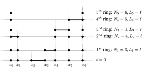
Figure 3: Example of a trajectory in $F_{k}$, with $k=5$.

Due to our previous considerations it holds

$$F_{k}=\bigcup_{\sigma\ \mathrm{admissible}}{\mathcal{B}}(\sigma),$$

where a string $\sigma=(\sigma_{1},\sigma_{2},\ldots,\sigma_{m})$ is called admissible if the following properties are satisfied: [(P2)]

if $L_{1}=\ell$, then $N_{1}\in[2,k+1]$; the numbers $N_{i}$ associated to the letter $\ell$ are all the integers in $[N_{1},k+1]$, and they appear in the string in increasing order; the numbers $N_{i}$ associated to the letter $r$ are all the positive integers in $[1,N_{1}-2]$, and they appear in the string in decreasing order;

if $L_{1}=r$, then $N_{1}\in[1,k]$, the numbers $N_{i}$ associated to the letter $\ell$ are all the integers in $[N_{1}+2,k+1]$, and they appear in the string in increasing order; the numbers $N_{i}$ associated to the letter $r$ are all the integers in $[1,N_{1}]$, and they appear in the string in decreasing order. Observe that an admissible string must have $k$ entries, that is, $m=k$, and that the knowledge of $(L_{i})_{1\leq i\leq k}$ allows to determine uniquely the numbers $(N_{i})_{1\leq i\leq k}$.

Recall that ${\lambda}^{*}_{\ell}(d)={\lambda}_{r}(d)$, ${\lambda}_{r}^{*}(d)={\lambda}_{\ell}(d)$. Writing $d_{i}(0)$ as $d_{i}$ (for simplicity of notation), if $\sigma$ is admissible we get

$${\mathbb{E}}_{\otimes_{k+1}\mu}\bigl{[}e^{-sd_{1}(\infty)};{\mathcal{B}}(\sigma)\bigr{]}={\mathbb{E}}_{\otimes_{k+1}\mu}[F(d_{1},d_{2},\ldots,d_{k+1},\sigma)],$$ (45)

where

$$F(d_{1},d_{2},\ldots,d_{k+1},\sigma)$$

$$\qquad=\Biggl{(}\prod_{i=1}^{k+1}e^{-sd_{i}}\mathbh{1}_{d_{i}\in{\mathcal{A}}}\Biggr{)}\frac{{\lambda}(d_{N_{1}})}{{\lambda}(d_{1})+\cdots+{\lambda}(d_{k+1})}$$

(46)

$$\qquad\quad{}\times\frac{{\lambda}^{*}_{L_{1}}(d_{N_{1}})}{{\lambda}(d_{N_{1}})}\prod_{i=2}^{k}\frac{{\lambda}(d_{N_{i}})}{\sum_{j=i}^{k}{\lambda}(d_{N_{j}})}\frac{{\lambda}^{*}_{L_{i}}(d_{N_{i}})}{{\lambda}(d_{N_{i}})}$$

$$\qquad=\Biggl{(}\prod_{i=1}^{k+1}e^{-sd_{i}}\mathbh{1}_{d_{i}\in{\mathcal{A}}}\Biggr{)}\frac{{\lambda}^{*}_{L_{1}}(d_{N_{1}})}{{\lambda}(d_{1})+\cdots+{\lambda}(d_{k+1})}\prod_{i=2}^{k}\frac{{\lambda}^{*}_{L_{i}}(d_{N_{i}})}{\sum_{j=i}^{k}{\lambda}(d_{N_{j}})}$$

(the last factor is defined as $1$ if $k=1$).

Observe that the law $\otimes_{k+1}\mu$ is exchangeable, that is, it is left invariant by permutations of $d_{1},d_{2},\ldots,d_{k+1}$. This symmetry leads to the identity

$${\mathbb{E}}_{\otimes_{k+1}\mu}[F(d_{1},d_{2},\ldots,d_{k+1},\sigma)]={\mathbb{E}}_{\otimes_{k+1}\mu}[G(d_{1},d_{2},\ldots,d_{k+1},(L_{i})_{1\leq i\leq k})],$$

where

$$G(d_{1},d_{2},\ldots,d_{k+1},(L_{i})_{1\leq i\leq k})$$

$$\qquad=\Biggl{(}\prod_{i=1}^{k+1}e^{-sd_{i}}\mathbh{1}_{d_{i}\in{\mathcal{A}}}\Biggr{)}\frac{{\lambda}^{*}_{L_{1}}(d_{1})}{{\lambda}(d_{1})+\cdots+{\lambda}(d_{k+1})}\prod_{i=2}^{k}\frac{{\lambda}^{*}_{L_{i}}(d_{i})}{\sum_{j=i}^{k}{\lambda}(d_{j})}.$$

Recall that an admissible string $\sigma$ is uniquely determined by its letter string $(L_{i})_{1\leq i\leq k}$, and observe that each string in $\{\ell,r\}^{[1,k]}$ is the letter string $(L_{i})_{1\leq i\leq k}$ for some admissible $\sigma$. Therefore we have

$${\mathbb{E}}_{\otimes_{k+1}\mu}\bigl{[}e^{-sd_{1}(\infty)};F_{k}\bigr{]}$$

$$\qquad=\sum_{\sigma\ \mathrm{admissible}}{\mathbb{E}}_{\otimes_{k+1}\mu}[F(d_{1},d_{2},\ldots,d_{k+1},\sigma)]$$

(47)

$$\qquad=\sum_{L_{1},\ldots,L_{k}\in\{\ell,r\}}{\mathbb{E}}_{\otimes_{k+1}\mu}[G(d_{1},d_{2},\ldots,d_{k+1},(L_{i})_{1\leq i\leq k})]$$

$$\qquad={\mathbb{E}}_{\otimes_{k+1}\mu}[H(d_{1},d_{2},\ldots,d_{k+1})],$$

where

$$H(d_{1},d_{2},\ldots,d_{k+1})=\Biggl{(}\prod_{i=1}^{k+1}e^{-sd_{i}}\mathbh{1}_{d_{i}\in{\mathcal{A}}}\Biggr{)}\frac{{\lambda}(d_{1})}{{\lambda}(d_{1})+\cdots+{\lambda}(d_{k+1})}\prod_{i=2}^{k}\frac{{\lambda}(d_{i})}{\sum_{j=i}^{k}{\lambda}(d_{j})}.$$

Applying Lemma E.1 in Appendix E with $k+1$ instead of $k$, $m=\mu$, $f(x)=e^{-sx}\mathbh{1}_{x\in{\mathcal{A}}}$ and $g(x)={\lambda}(x)$, we end up with

$${\mathbb{E}}_{\otimes_{k+1}\mu}[H(d_{1},\ldots,d_{k+1})]=\frac{1}{(k+1)\cdot(k-1)!}\biggl{[}\int\mu(dx)e^{-sx}\mathbh{1}_{x\in{\mathcal{A}}}\biggr{]}^{k+1}.\vspace*{-2pt}$$ (48)

This ends the proof of Lemma 4.1. Proof of Lemma 4.2 The proof follows the main arguments in the proof of Lemma 4.1, hence we skip some details. As in the proof of Lemma 4.1 we work with the one-epoch coalescence process with law ${\mathbb{P}}_{\otimes_{k+1}\mu}$.

Denoting the jumps of the coalescence process (disregarding the jump times) with the same rule used in the proof of Lemma 4.1, that is, by means of the string $\sigma$, we get that

$$E_{k,j}=\bigcup_{\sigma\ j\mbox{-}\mathrm{admissible}}{\mathcal{B}}(\sigma),\vspace*{-2pt}$$ (49)

where now $j$-admissible means that the numbers $N_{i}$ associated to the letter $\ell$ appear in the string $\sigma$ in increasing order from $j+1$ to $k+1$, while the numbers $N_{i}$ associated to the letter $r$ appear in the string $\sigma$ in decreasing order from $j-1$ to $1$. Note that in particular $\sigma$ contains $j-1$ letters “$r$” and “$k+1-j$” letters $\ell$, and therefore $\sigma$ has length $k$.

As in the previous proof we set $d_{r}=d_{r}(0)$. We then compute the expectation

$${\mathbb{E}}_{\otimes_{k+1}\mu}\bigl{[}e^{-sd_{1}(\infty)};{\mathcal{B}}(\sigma)\bigr{]}$$

$$\qquad={\mathbb{E}}_{\otimes_{k+1}\mu}\Biggl{[}e^{-sd_{j}}\mathbh{1}_{d_{j}\notin{\mathcal{A}}}\prod_{i=1}^{k}\biggl{\{}e^{-sd_{N_{i}}}\mathbh{1}_{d_{N_{i}}\in{\mathcal{A}}}\frac{{\lambda}^{*}_{L_{i}}(d_{N_{i}})}{\sum_{r=i}^{k}{\lambda}(d_{N_{r}})}\biggr{\}}\Biggr{]}$$

(50)

$$\qquad={\mathbb{E}}_{\otimes_{k+1}\mu}\Biggl{[}e^{-sd_{k+1}}\mathbh{1}_{d_{k+1}\notin{\mathcal{A}}}\prod_{i=1}^{k}\biggl{\{}e^{-sd_{i}}\mathbh{1}_{d_{i}\in{\mathcal{A}}}\frac{{\lambda}^{*}_{L_{i}}(d_{i})}{\sum_{r=i}^{k}{\lambda}(d_{r})}\biggr{\}}\Biggr{]}$$

$$\qquad=\biggl{(}\int e^{-sx}\mathbh{1}_{x\notin{\mathcal{A}}}\mu(dx)\biggr{)}{\mathbb{E}}_{\otimes_{k}\mu}\Biggl{[}\prod_{i=1}^{k}\biggl{\{}e^{-sd_{i}}\mathbh{1}_{d_{i}\in{\mathcal{A}}}\frac{{\lambda}^{*}_{L_{i}}(d_{i})}{\sum_{r=i}^{k}{\lambda}(d_{r})}\biggr{\}}\Biggr{]},\vspace*{-2pt}$$

where in the second identity we have used the exchangeability of $\otimes_{k+1}\mu$, and in the third identity we have simply factorized the probability measure.

Summing over $j$ allows us to remove the constraint that $\sigma$ must have $j-1$ letters “$r$” and “$k+1-j$” letters $\ell$, hence

$$\sum_{j=1}^{k+1}{\mathbb{E}}_{\otimes_{k+1}\mu}\bigl{[}e^{-sd_{1}(\infty)};E_{k,j}\bigr{]}$$

$$\qquad=\sum_{L_{1},\ldots,L_{k}\in\{\ell,r\}}\mbox{ r.h.s. of (\ref{fornaciari})}$$

$$\qquad=\biggl{(}\int e^{-sx}\mathbh{1}_{x\notin{\mathcal{A}}}\mu(dx)\biggr{)}{\mathbb{E}}_{\otimes_{k}\mu}\Biggl{[}\prod_{i=1}^{k}\biggl{\{}e^{-sd_{i}}\mathbh{1}_{d_{i}\in{\mathcal{A}}}\frac{{\lambda}(d_{i})}{\sum_{r=i}^{k}{\lambda}(d_{r})}\biggr{\}}\Biggr{]}.$$

Applying point (b) of Lemma E.1 [with $f(x)=e^{-sx}\mathbh{1}_{x\in{\mathcal{A}}}$ and $g(x)={\lambda}(x)$] completes the proof of Lemma 4.2.

4.1 Proof of Theorem 2.14(ii)

The proof of point (ii)(a) is trivial, since ${\lambda}_{r}\equiv 0$, then $x_{0}(t)=x_{0}(0)$ for any time $t\geq 0$. Indeed the first point $x_{0}(t)$ of $\xi(t)$ cannot be erased from the left due the infinite domain, and from the right due to the assumption ${\lambda}_{r}\equiv 0$.

We now concentrate on point (ii)(b). Due to (37), we can write (for $s\in{\mathbb{R}}_{+}\cup i{\mathbb{R}}$)

$$L_{\infty}(s)={\mathbb{P}}_{\operatorname{Ren}({\delta}_{0},\nu)}\bigl{(}0\in\xi(\infty)\bigr{)}L_{0}(s)\sum_{k=0}^{\infty}B_{k}(s),$$ (52)

where $B_{k}(s)={\mathbb{E}}_{\otimes_{k}\mu}(e^{-sx_{k}(0)};\xi(\infty)=\{x_{k}(0)\})$.

Lemma 4.3

$B_{0}(s)=1$ while, for any $k\geq 1$, it holds

$$B_{k}(s)=\mathbb{E}_{\otimes_{k}\mu}\Biggl{(}\prod_{i=1}^{k}e^{-sd_{i}}\frac{{\lambda}_{\ell}^{*}(d_{i})\mathbh{1}_{d_{i}\in\mathcal{A}}}{\sum_{j=i}^{k}{\lambda}(d_{j})}\Biggr{)}.$$ (53)

We work with the one-epoch coalescence process with law ${\mathbb{P}}_{\otimes_{k}\mu}$. The case $k=0$ is trivial. We take $k\geq 1$. Due to the blocking phenomenon, there is only one possible way to realize the event $\{\xi(\infty)=x_{k}(0)\}$: only the points $x_{0}(0),x_{1}(0),\ldots,x_{k-1}(0)$ must disappear, one after the other from the left to the right. Setting $d_{i}=d_{i}(0)$, this implies that $d_{1},\ldots,d_{k}$ belong to ${\mathcal{A}}$. In this case, knowing $\xi(0)$, the above event has probability

$$\frac{{\lambda}_{\ell}^{*}(d_{1})}{\sum_{j=1}^{k}{\lambda}(d_{j})}\times\frac{{\lambda}_{\ell}^{*}(d_{2})}{\sum_{j=2}^{k}{\lambda}(d_{j})}\times\cdots\times\frac{{\lambda}_{\ell}^{*}(d_{k})}{{\lambda}(d_{k})}=\prod_{i=1}^{k}\frac{{\lambda}_{\ell}^{*}(d_{i})}{\sum_{j=i}^{k}{\lambda}(d_{j})}.$$

Since $x_{k}(0)=d_{1}+d_{2}+\cdots+d_{k}$, we get (53).

Since $\lambda_{\ell}=\gamma\lambda_{r}$ we have ${\lambda}_{r}^{*}=\gamma{\lambda}_{\ell}^{*}$. In particular ${\lambda}={\lambda}_{\ell}^{*}+{\lambda}_{r}^{*}=(1+\gamma){\lambda}_{\ell}^{*}$. Hence, due to (52) and Lemma 4.3, we get

$$L_{\infty}(s)=CL_{0}(s)\sum_{k=0}^{\infty}\frac{1}{(1+\gamma)^{k}}{\mathbb{E}}_{\otimes_{k}\mu}\Biggl{(}\prod_{i=1}^{k}e^{-sd_{i}}\frac{\lambda(d_{i})\mathbh{1}_{d_{i}\in\mathcal{A}}}{\sum_{j=i}^{k}{\lambda}(d_{j})}\Biggr{)},$$

where $C:={\mathbb{P}}_{\operatorname{Ren}({\delta}_{0},\nu)}(0\in\xi(\infty))$ and where, in the last series, the addendum with $k=0$ is defined as $1$. Applying point (b) of Lemma E.1 [with $f(x)=e^{-sx}\mathbh{1}_{x\in\mathcal{A}}$ and $g(x)={\lambda}(x)$], and recalling that $H_{0}(s)=\int e^{-sx}\mathbh{1}_{x\in\mathcal{A}}\mu(dx)$, we end up with

$$L_{\infty}(s)=CL_{0}(s)\sum_{k=0}^{\infty}\frac{H_{0}(s)^{k}}{(1+\gamma)^{k}\cdot k!}=CL_{0}(s)\exp\biggl{\{}\frac{H_{0}(s)}{1+\gamma}\biggr{\}}.$$

Since $L_{0}(0)=L_{\infty}(0)=1$, the latter identity applied to $s=0$ leads to $C=\exp\{-\frac{H_{0}(0)}{1+\gamma}\}$ which in turn leads to (12). Then (13) follows immediately by noticing that ${\mathbb{P}}_{\operatorname{Ren}(\nu,\mu)}(x_{0}(0)\in\xi(\infty))={\mathbb{P}}_{\operatorname{Ren}(\delta_{0},\mu)}(0\in\xi(\infty))$ and from the above definition of $C$.

5 Analysis of the recursive identity (11) in OCP

As mentioned in the Introduction, a crucial tool to prove Theorem 2.19 is given by a special integral representation of certain Laplace transforms, which makes identities (11) and (12) finally treatable. We first consider (11), focusing our attention on the one-epoch coalescence process in the same setting of Section 2 (i.e., the active domains have length in $[d_{\min},d_{\max})$). In what follows, we present an overview of the global scheme, postponing proofs to the end of the section. It is convenient to work with rescaled random variables. More precisely, in the same setting of Theorem 2.13, we call $X_{0},X_{\infty}$ some generic random variables with law $\mu,\mu_{\infty}$, respectively. Then we define

$$Z_{0}=X_{0}/d_{\min}\quad\mbox{and}\quad Z_{\infty}=X_{\infty}/d_{\max}$$

as the rescaled random variables. Setting for $s>0$

$$g_{0}(s) = {\mathbb{E}}(e^{-sZ_{0}}),\qquad g_{\infty}(s)={\mathbb{E}}(e^{-sZ_{\infty}}),$$

$$h_{0}(s) = {\mathbb{E}}(e^{-sZ_{0}};Z_{0}<a),\qquad a=\frac{d_{\max}}{d_{\min}},$$

equation (11) becomes equivalent to

$$1-g_{\infty}(as)=\bigl{(}1-g_{0}(s)\bigr{)}e^{h_{0}(s)}.$$ (55)

By definition, and because of assumption (A2), we have $Z_{0}\geq 1$, $Z_{\infty}\geq 1$ and $a\in[1,2]$. These bounds will turn out to be crucial later on.

For later use, we point out some simple identities. We recall the definition of the exponential integral function $\operatorname{Ei}(s)$, $s>0$,

$$\operatorname{Ei}(s)=\int_{s}^{\infty}\frac{e^{-t}}{t}\,dt=\int_{1}^{\infty}\frac{e^{-sx}}{x}\,dx.$$

Given a Radon measure $t$ on $[0,\infty)$ (i.e., a Borel nonnegative measure, giving finite mass to any bounded Borel set), by Fubini’s theorem it is simple to check that

$$\int_{0}^{\infty}\frac{e^{-s(1+x)}}{1+x}t(dx)=\int_{s}^{\infty}du\,e^{-u}\int_{0}^{\infty}e^{-ux}t(dx).$$ (56)

Above and in what follows, we will write $\int_{c}^{\infty}$ instead of $\int_{[c,\infty)}$ for $c\geq 0$. If $t(dx)=c_{0}\,dx$, the quantity in (56) is simply the exponential integral $\operatorname{Ei}(s)$ and the right-hand side of (56) gives an alternative integral representation of $\operatorname{Ei}(s)$. In particular, the limit points in Theorem 2.19 have Laplace transform of the form

$$g_{\infty}^{(c_{0})}(s) = 1-\exp\biggl{\{}-\int_{0}^{\infty}\frac{e^{-s(1+x)}}{1+x}t(dx)\biggr{\}}$$

$$= 1-\exp\biggl{\{}-\int_{s}^{\infty}du\,e^{-u}\int_{0}^{\infty}e^{-ux}t(dx)\biggr{\}},$$

where $t(dx)=c_{0}\,dx$.

This observation suggests to write the Laplace transforms $g_{0}$, $g_{\infty}$ in the form (5) for suitable Radon measures $t_{0}$ and $t_{\infty}$. The following result guarantees that such an integral representation exists.

Lemma 5.1

Let $Z$ be a random variable such that $Z\geq 1$, and define $g(s)={\mathbb{E}}[e^{-sZ}]$, $s\geq 0$. Let $w\dvtx(0,\infty)\rightarrow{\mathbb{R}}$ be the unique function such that

$$g(s)=1-\exp\biggl{\{}-\int_{s}^{\infty}du\,e^{-u}w(u)\biggr{\}},\qquad s>0,$$ (58)

that is,

$$w(s)=-\frac{e^{s}g^{\prime}(s)}{1-g(s)},\qquad s>0.$$ (59)

Then the function $w$ is completely monotone. In particular, there exists a unique Radon measure $t(dx)$ on $[0,\infty)$ (not necessarily of finite total mass) such that

$$w(s)=\int_{0}^{\infty}e^{-sx}t(dx),\qquad s>0,$$ (60)

and therefore

$$g(s)=1-\exp\biggl{\{}-\int_{0}^{\infty}\frac{e^{-s(1+x)}}{1+x}t(dx)\biggr{\}},\qquad s\geq 0.$$ (61)

Moreover,

$$\limsup_{s\downarrow 0}-\frac{sg^{\prime}(s)}{1-g(s)}\in[0,1].$$ (62)

We recall that a function $f\dvtx(0,\infty)\rightarrow{\mathbb{R}}$ is called completely monotone if it possesses derivatives $D^{n}f$ of all orders and

$$(-1)^{n}D^{n}f(x)\geq 0\qquad\forall x>0.$$

Due to the above lemma, there exist two uniquely determined Radon measures $t_{0}$ and $t_{\infty}$ on $[0,\infty)$, such that $g_{0}$ and $g_{\infty}$ admit the integral representation (61) with $t$ replaced by $t_{0}$ and $t_{\infty}$, respectively.

In order to rewrite (55) as identity in terms of $t_{0}$ and $t_{\infty}$, we need to express the function $h_{0}$ in terms of $t_{0}$. The following result gives us the solution:

Lemma 5.2

Let $Z$ be a random variable such that $Z\geq 1$, and let $g(s)$ be its Laplace transform. Let $t$ be the unique Radon measure on $[0,\infty)$ satisfying (61) and call $m(dx)$ the Radon measure with support in $[1,\infty)$ such that

$$m(A)=\int_{0}^{\infty}\frac{\mathbh{1}_{1+x\in A}}{1+x}t(dx).$$ (63)

For each $k\geq 1$, consider the convolution measure $m^{(k)}$ with support in $[k,\infty)$ defined as

$$m^{(k)}(A)=\int_{1}^{\infty}m(dx_{1})\int_{1}^{\infty}m(dx_{2})\cdots\int_{1}^{\infty}m(dx_{k})\mathbh{1}_{x_{1}+x_{2}+\cdots+x_{k}\in A}.$$ (64)

Then the law of $Z$ is given by

$$\sum_{k=1}^{\infty}\frac{(-1)^{k+1}}{k!}m^{(k)}.$$ (65)

In particular

$${\mathbb{E}}[e^{-sZ};Z<a]=\int_{[0,a-1)}\frac{e^{-s(1+x)}}{1+x}t(dx),\qquad s\geq 0.$$ (66)

We point out that, given a bounded Borel set $A$, the series

$$m_{*}(A)=\sum_{k=1}^{\infty}\frac{(-1)^{k+1}}{k!}m^{(k)}(A)$$

is a finite sum, since $m^{(k)}$ has support in $[k,\infty)$. The thesis includes that this sum is a nonnegative number and that the set-function $A\mapsto m_{*}(A)$, defined on bounded Borel sets, extend uniquely to a Radon measure on all Borel sets.

Equation (66) above allows us to write $h_{0}(s)$ in terms of $t_{0}$. Collecting the above observations we get for $s\geq 0$

$$g_{0}(s) = 1-\exp\biggl{\{}-\int_{0}^{\infty}\frac{e^{-s(1+x)}}{1+x}t_{0}(dx)\biggr{\}},$$

$$g_{\infty}(s) = 1-\exp\biggl{\{}-\int_{0}^{\infty}\frac{e^{-s(1+x)}}{1+x}t_{\infty}(dx)\biggr{\}},$$

$$h_{0}(s) = \int_{[0,a-1)}\frac{e^{-s(1+x)}}{1+x}t_{0}(dx).$$

Due to the above identities, (55) is equivalent to

$$\qquad\int_{0}^{\infty}\frac{e^{-as(1+x)}}{1+x}t_{\infty}(dx)=\int_{[a-1,\infty)}\frac{e^{-s(1+x)}}{1+x}t_{0}(dx),\qquad s\geq 0.$$ (67)

It is convenient now to introduce the following notation. Given an increasing function $\phi\dvtx[0,\infty)\rightarrow[0,\infty)$ and a Radon measure $\mathfrak{m}$ on $[0,\infty)$, we denote by $\mathfrak{m}\circ\phi$ the new Radon measure on $[0,\infty)$ defined by

$$\mathfrak{m}\circ\phi(A)=\mathfrak{m}(\phi(A)),\qquad A\subset{\mathbb{R}}\mbox{ Borel}.$$ (68)

Note that $\mathfrak{m}\circ\phi$ is indeed a measure, due to the injectivity of $\phi$. Moreover, it holds

$$\int_{0}^{\infty}f(x)\mathfrak{m}\circ\phi(dx)=\int_{[\phi(0),\infty)}f(\phi^{-1}(x))\mathfrak{m}(dx).$$ (69)

We are finally able to give a simple characterization of (67), which we know to be equivalent to (55):

Theorem 5.3

Consider the linear function $\phi\dvtx[0,\infty)\rightarrow[0,\infty)$ defined as $\phi(x)=a(1+x)-1$. Then, equation (67) [and therefore also (55)] is equivalent to the relation

$$t_{\infty}=(1/a)t_{0}\circ\phi.$$ (70)

5.1 Proof of Lemma 5.1

First we prove that $w$ is a completely monotone function. Since $g(s)<1$ for $s>0$, we can write $w=f\sum_{k=0}^{\infty}g^{k}$ where $f(s)=-e^{s}g^{\prime}(s)$. Trivially, $g$ is a completely monotone function. Since the product of completely monotone functions is again a completely monotone function (see Criterion 1 in Section XIII.4 of Fe2 ), we conclude that $g^{k}$ is a completely monotone function. Since the sum of completely monotone functions is trivially completely monotone, we conclude that $\sum_{k=0}^{\infty}g^{k}$ is completely monotone. It remains to prove that $f$ is completely monotone. To this aim we observe that, by the Leibniz rule,

$$D^{n}f(s) = -\sum_{k=0}^{n}\pmatrix{n\cr k}D^{n-k}(e^{s})D^{k}(g^{\prime}(s))=-e^{s}\sum_{k=0}^{n}\pmatrix{n\cr k}D^{k+1}g(s)$$

$$= -e^{s}\sum_{k=0}^{n}\pmatrix{n\cr k}(-1)^{k+1}{\mathbb{E}}(e^{-sZ}Z^{k+1})=e^{s}{\mathbb{E}}\Biggl{(}e^{-sZ}Z\sum_{k=0}^{n}\pmatrix{n\cr k}(-Z)^{k}\Biggr{)}$$

$$= e^{s}{\mathbb{E}}\bigl{(}e^{-sZ}Z(1-Z)^{n}\bigr{)}.$$

Since $1-Z\leq 0$, the sign of the $n$th derivative $D^{n}f$ is $(-1)^{n}$.

At this point, we can apply Theorem 1a in Section XIII.4 of Fe2 to get that there exists a Radon measure $t(dx)$ on $[0,\infty)$ (not necessarily of finite total mass) satisfying (60). Moreover, the above measure $t$ is uniquely determined due to the inversion formula given in Theorem 2, Section XIII.4 of Fe2 . Finally, we derive (61) for $s>0$ from (56), (58) and (60). The extension to $s=0$ follows from the monotone convergence theorem.

In order to prove (62) we observe that $ye^{-y}\leq 1-e^{-y}$ for all $y\geq 0$, thus implying that

$$-sg^{\prime}(s)={\mathbb{E}}(sZe^{-sZ})\leq 1-{\mathbb{E}}(e^{-sZ})=1-g(s)\qquad\forall s>0.$$

In particular, the ratio in (62) is bounded by $1$. On the other hand $-sg^{\prime}(s)={\mathbb{E}}(sZe^{-sZ})>0$ while $1-g(s)>0$, thus implying that the ratio in (62) is positive.

5.2 Proof of Lemma 5.2

Due to the definition of $m(dx)$, we can write

$$\int_{0}^{\infty}\frac{e^{-s(1+x)}}{1+x}t(dx)=\int_{0}^{\infty}e^{-sx}m(dx).$$ (71)

By (61), since $g(s)<1$ for $s>0$, we get that the above quantities are finite as $s>0$. Using the series expansion of the exponential function we can write

$$\qquad 1-\exp\biggl{\{}-\int_{0}^{\infty}\frac{e^{-s(1+x)}}{1+x}t(dx)\biggr{\}}=\sum_{k=1}^{\infty}\frac{(-1)^{k+1}}{k!}\biggl{(}\int_{0}^{\infty}e^{-sx}m(dx)\biggr{)}^{k}.$$ (72)

Since

$$\biggl{(}\int_{0}^{\infty}e^{-sx}m(dx)\biggr{)}^{k}=\int_{0}^{\infty}e^{-sx}m^{(k)}(dx),$$ (73)

we can rewrite (72) as

$$\sum_{k=1}^{\infty}\frac{(-1)^{k+1}}{k!}\int_{0}^{\infty}e^{-sx}m^{(k)}(dx)=\sum_{k=1}^{\infty}\Biggl{(}\sum_{j=k}^{\infty}a_{k,j}\Biggr{)},$$ (74)

where

$$a_{k,j}=\frac{(-1)^{k+1}}{k!}\int_{I_{j}}e^{-sx}m^{(k)}(dx),\qquad I_{j}=[j,j+1)\qquad\mbox{for }j\geq 1.$$

Using again the series expansion of the exponential function and also (73), we conclude that

$$\sum_{k=1}^{\infty}\sum_{j=1}^{\infty}|a_{j,k}| = \sum_{k=1}^{\infty}\frac{1}{k!}\int_{0}^{\infty}e^{-sx}m^{(k)}(dx)$$

$$= \exp\biggl{\{}\int_{0}^{\infty}e^{-sx}m(dx)\biggr{\}}-1<\infty.$$

In particular, we can arrange arbitrarily the terms in the series given by the right-hand side of (74), getting always the same limit. This fact implies that

$$\qquad\mbox{r.h.s. of }(\ref{tacchi}) = \sum_{j=1}^{\infty}\Biggl{(}\sum_{k=1}^{j}a_{k,j}\mathbh{1}_{k\ \mathrm{odd}}\Biggr{)}+\sum_{j=1}^{\infty}\Biggl{(}\sum_{k=1}^{j}a_{k,j}\mathbh{1}_{k\ \mathrm{even}}\Biggr{)}$$

$$= \int_{0}^{\infty}e^{-sx}\nu_{+}(dx)-\int_{0}^{\infty}e^{-sx}\nu_{-}(dx),$$

where the Radon measures $\nu_{+}$ and $\nu_{-}$ on $[0,\infty)$ are defined as follows:

$$\nu_{+}(A) = \sum_{k=1}^{\infty}\frac{\mathbh{1}_{k\ \mathrm{odd}}}{k!}m^{(k)}(A),$$

$$\nu_{-}(A) = \sum_{k=1}^{\infty}\frac{\mathbh{1}_{k\ \mathrm{even}}}{k!}m^{(k)}(A).$$

We point out that for any bounded Borel subset $A\subset[0,\infty)$ the above series are indeed finite sums since each $m^{(k)}$ has support in $[k,\infty)$. In addition, $\nu_{+}$ and $\nu_{-}$ have support contained in $[1,\infty)$ and $[2,\infty)$, respectively.

Collecting (61), (72), (74) and (5.2), we obtain that

$$g(s)=\int_{0}^{\infty}e^{-sx}\nu_{+}(dx)-\int_{0}^{\infty}e^{-sx}\nu_{-}(dx)$$

for all $s>0$. Writing $p_{Z}$ for the law of $Z$, the above identity implies that the Laplace transforms of the measures $p_{Z}+\nu_{-}$ and $\nu_{+}$ coincide on $(0,\infty)$. Due to Theorem 2 in Section XIII.4 of Fe2 , this implies that $p_{Z}+\nu_{-}=\nu_{+}$. It follows that

$$p_{Z}(A)=\nu_{+}(A)-\nu_{-}(A)\qquad\forall A\subset{\mathbb{R}}\mbox{ bounded and Borel}.$$

Since for $A$ as above we can write $\nu_{+}(A)-\nu_{-}(A)=\sum_{k=1}^{\infty}\frac{(-1)^{k+1}}{k!}m^{(k)}(A)$, we get that the law $p_{Z}$ coincides with (65).

It remains now to prove (66). To this aim we observe that, since $m^{(k)}$ has support contained in $[k,\infty)$, measure (65) equals $m$ on $[1,2)$. Since $a\leq 2$, and using the definition of the measure $m$ given by (63), we obtain that

$${\mathbb{E}}[e^{-sZ};Z<a] = \int_{[1,a)}e^{-sx}p_{Z}(dx)=\int_{[1,a)}e^{-sx}m(dx)$$

$$= \int_{[0,a-1)}\frac{e^{-s(1+x)}}{1+x}t(dx).$$

This concludes the proof of (66).

5.3 Proof of Theorem 5.3

We write $\rho(dx)$ for the measure in the right-hand side of (70). Using that $a[\phi^{-1}(x)+1]=1+x$, we obtain for $s\geq 0$ that

$$\int_{0}^{\infty}\frac{e^{-as(1+x)}}{1+x}\rho(dx) = a^{-1}\int_{[\phi(0),\infty)}\frac{e^{-s(1+x)}}{a^{-1}(1+x)}t_{0}(dx)$$

$$= \int_{[a-1,\infty)}\frac{e^{-s(1+x)}}{1+x}t_{0}(dx).$$

The above identity implies that (67) holds if and only if

$$\int_{0}^{\infty}\frac{e^{-as(1+x)}}{1+x}t_{\infty}(dx)=\int_{0}^{\infty}\frac{e^{-as(1+x)}}{1+x}\rho(dx)\qquad\forall s\geq 0.$$ (77)

We write $m_{\infty}$ and $m^{\prime}$ for the measures on $[1,\infty)$ such that

$$m_{\infty}(A)=\int_{0}^{\infty}\frac{\mathbh{1}_{1+x\in A}}{1+x}t_{\infty}(dx),\qquad m^{\prime}(A)=\int_{0}^{\infty}\frac{\mathbh{1}_{1+x\in A}}{1+x}\rho(dx)$$

for bounded Borel subsets $A\subset[1,\infty)$. Then, by (77), we get that (67) holds if and only if the Laplace transforms of the measures $m_{\infty}$ and $m^{\prime}$ coincide on $(0,\infty)$. By Theorem 2 in Section XIII.4 of Fe2 , this last property is equivalent to the identity $m_{\infty}=m^{\prime}$, which is equivalent to $t_{\infty}=\rho$.

6 Hierarchical Coalescence Process: Proofs

6.1 Application of the recursive identity (11) to the HCP

We begin by collecting some useful formulae for the hierarchical coalescence process that we derive from results obtained for the one-epoch coalescence process in the previous section. These formula will be used throughout the whole section.

We use notation and definitions of Theorem 2.19. In particular $\mu$ and $\nu$ are probability measures on $[1,\infty)$ and $\mathbb{R}$, respectively. We define here $X^{(n)}$, $n\in{\mathbb{N}}_{+}$, as the length of the leftmost domain inside $(0,\infty)$ at the beginning of the $n$th epoch, that is, $X^{(n)}=x^{(n)}_{2}(0)-x^{(n)}_{1}(0)$. Moreover we set $Z^{(n)}=X^{(n)}/d^{(n)}$. Note that $X^{(n)}$ has law $\mu^{(n)}$. Also, $\mathbb{E}$ stands for the expectation with respect to the hierarchical coalescent process starting indifferently from ${\mathcal{Q}}=\operatorname{Ren}(\nu,\mu)$, ${\mathcal{Q}}=\operatorname{Ren}(\mu)$ or ${\mathcal{Q}}=\operatorname{Ren}_{\mathbb{Z}}(\mu)$. For any $n\in\mathbb{N}_{+}$ and any $s\geq 0$ let

$$g^{(n)}(s)=\mathbb{E}\bigl{(}e^{-sZ^{(n)}}\bigr{)},\qquad h^{(n)}(s)=\mathbb{E}\bigl{(}e^{-sZ^{(n)}}\mathbh{1}_{1\leq Z^{(n)}<a_{n}}\bigr{)},$$ (78)

where $a_{n}=d^{(n+1)}/d^{(n)}$. Thanks to Theorem 2.13, [see also (55)], we get a system of recursive identities

$$1-g^{(n)}(sa_{n-1})=\bigl{(}1-g_{n-1}(s)\bigr{)}e^{h^{(n-1)}(s)}\qquad\forall n\geq 2.$$ (79)

These recursive identities will be essential in the subsequent computations. Since $Z^{(n)}\geq 1$, by Lemma 5.1 there exists a unique measure $t^{(n)}$ on $[0,\infty)$ such that

$$g^{(n)}(s)=1-\exp\biggl{\{}-\int_{0}^{\infty}\frac{e^{-s(1+x)}}{1+x}t^{(n)}(dx)\biggr{\}},\qquad n\geq 1.$$ (80)

Invoking now Theorem 5.3 we conclude that

$$t^{(n)}=(1/a_{n-1})t^{(n-1)}\circ\phi_{n-1},\qquad n\geq 2,$$ (81)

where $\phi_{n}(x)=a_{n}(1+x)-1$.

Up to now we have only moved from the system of recursive identities (79) to the new system (81). But while the former is highly nonlinear and complex, the latter is solvable. Indeed if we define

$$\psi_{n}(x):=\phi_{1}\circ\phi_{2}\circ\cdots\circ\phi_{n}(x),$$ (82)

then $\psi_{n}(x)=d^{(n+1)}(1+x)-1$ and (68) together with (81) imply

$$t^{(n)}=\frac{1}{d^{(n)}}t^{(1)}\circ\psi_{n-1},\qquad n\geq 2.$$ (83)

Finally, using (66) and (83), it is simple to check that

$$h^{(n)}(s)=\int_{[d^{(n)}-1,d^{(n+1)}-1)}e^{-s(1+x)/d^{(n)}}(1+x)^{-1}t^{(1)}(dx),\qquad n\geq 1,$$ (84)

where we used the identity $(1+\psi^{-1}_{n-1}(x))=(1+x)/d^{(n)}$.

6.2 Asymptotic of the interval law in the HCP: Proof of Theorem 2.19

Section 6.1 provides us with most of the tools necessary for the proof of Theorem 2.19. In particular our starting point is identity (80):

$$g^{(n)}(s)=1-\exp\biggl{\{}-\int_{0}^{\infty}\frac{e^{-s(1+x)}}{1+x}t^{(n)}(dx)\biggr{\}},\qquad n\geq 1.$$ (85)

Defining

$$U^{(n)}(x)=\cases{t^{(n)}([0,x]),&\quad if $x\geq 0$,\cr 0,&\quad otherwise,}$$ (86)

we get that $U^{(n)}$ is a càdlàg function, $dU^{(n)}=t^{(n)}$ and $U^{(n)}(x)=0$ for $x<0$. By (83) it holds that

$$U^{(n)}(x) = \frac{1}{d^{(n)}}\bigl{[}U^{(1)}(\psi_{n-1}(x))-U^{(1)}(\psi_{n-1}(0)-)\bigr{]},$$

$$= \frac{1}{d^{(n)}}\bigl{[}U^{(1)}\bigl{(}d^{(n)}(1+x)-1\bigr{)}-U^{(1)}\bigl{(}\bigl{(}d^{(n)}-1\bigr{)}-\bigr{)}\bigr{]},\qquad n\geq 1.$$

If we fix $n\geq 2$, integrate by parts and use $U^{(n)}(0-)=0$, we can rewrite the integral in (85) as

$$\int_{0}^{\infty}\frac{e^{-s(1+x)}}{1+x}t^{(n)}(dx) = \int_{0}^{\infty}\frac{e^{-s(1+x)}}{1+x}\,dU^{(n)}(x)$$

$$= \lim_{y\uparrow\infty}\frac{e^{-s(1+y)}}{1+y}U^{(n)}(y)$$

$${}-\int_{0}^{\infty}\biggl{(}\frac{d}{dx}\biggl{(}\frac{e^{-s(1+x)}}{1+x}\biggr{)}\biggr{)}U^{(n)}(x)\,dx.$$

We now use (17), the key hypothesis. Since $g^{(1)}(s)=g(s)$ because $d^{(1)}=1$, if $w^{(1)}$ denotes the Laplace transform of $t^{(1)}$ [i.e., $w^{(1)}(s)=\int_{0}^{\infty}e^{-sx}t^{(1)}(dx)$], then (17) together with (59) implies

$$\lim_{s\downarrow 0}sw^{(1)}(s)=c_{0}.$$ (89)

Finally, Tauberian Theorem 2 in Section XIII.5 of Fe2 shows that (89) gives

$$\lim_{y\uparrow\infty}\frac{U^{(1)}(y)}{y}=c_{0}.$$ (90)

The above limit together with (6.2) implies that there exists a suitable constant $C>0$ such that

$$U^{(n)}(x)\leq C(1+x),\qquad n\geq 1,x\geq 0.$$ (91)

In particular, the limit in the right-hand side of (6.2) is zero and

$$\int_{0}^{\infty}\frac{e^{-s(1+x)}}{1+x}t^{(n)}(dx)=-\int_{0}^{\infty}\biggl{(}\frac{d}{dx}\biggl{(}\frac{e^{-s(1+x)}}{1+x}\biggr{)}\biggr{)}U^{(n)}(x)\,dx,$$ (93)

$$\eqntext{n\geq 2.}$$

By (6.2), (90) and the fact that $c_{n}\to\infty$, $\lim_{n\to\infty}U^{(n)}(x)\to c_{0}x$ for all $x\geq 0$. This limit together with (91) allows us to apply the dominated convergence theorem, to get that

$$\lim_{n\to\infty}\int_{0}^{\infty}\frac{e^{-s(1+x)}}{1+x}t^{(n)}(dx) = -c_{0}\int_{0}^{\infty}\biggl{(}\frac{d}{dx}\biggl{(}\frac{e^{-s(1+x)}}{1+x}\biggr{)}\biggr{)}x\,dx$$

$$= c_{0}\int_{0}^{\infty}\frac{e^{-s(1+x)}}{1+x}\,dx$$

(in the last identity we have simply integrated by parts). In conclusion we have shown that $g^{(n)}$ converges point-wise to the function $g^{(\infty)}_{c_{0}}$ defined as in (18). Since in addition $\lim_{s\downarrow 0}g^{(\infty)}_{c_{0}}(s)=1$, by Theorem 2 in Section XIII.1 of Fe2 , we conclude that $g^{(\infty)}_{c_{0}}$ is the Laplace transform of some nonnegative random variable $Z_{c_{0}}^{(\infty)}$ and that $Z^{(n)}$ weakly converges to $Z_{c_{0}}^{(\infty)}$.

Finally, Lemma 5.2 allows us to determine the law of $Z_{c_{0}}^{(\infty)}$. Indeed, the measure $m$ associated to $t(dx):=c_{0}\,dx$ by means of (63) is simply of the form $m(dx)=(c_{0}/x)\mathbh{1}_{x\geq 1}\,dx$. In particular $m^{(k)}(dx)=c_{0}^{k}\rho_{k}(x)\mathbh{1}_{x\geq k}\,dx$ with $\rho_{k}$ defined in (19). It remains then to apply (65).

Remark 6.1.

It is useful to observe that if the initial scale $d^{(1)}$ was different from one than necessarily $g(s)\neq g^{(1)}(s)$. However, and that is the reason why we could fix $d^{(1)}=1$, the limit (17) is invariant under rescaling the variable $s$ by a constant, that is, (17) for $g$ implies the same limit for $g^{(1)}$.

6.3 Asymptotic of the first point law in the HCP: Proof of Theorem 2.24

We first prove the result for the special case $\nu={\delta}_{0}$. We set

$$\ell^{(n)}(s)={\mathbb{E}}\bigl{[}\exp\bigl{\{}-sX^{(n)}_{0}/d^{(n)}\bigr{\}}\bigr{]},\qquad s\in{\mathbb{R}}_{+}.$$

Recall the notation of Section 6.1 and in particular the definition of the constants $a_{n}=d^{(n+1)}/d^{(n)}$. By applying to each epoch the key identity (12), we get the recursive system,

$$\ell^{(n)}(s)=\ell^{(n-1)}(s/a_{n-1})\exp\biggl{\{}\frac{1}{1+\gamma}\bigl{[}h^{(n-1)}(s/a_{n-1})-h^{(n-1)}(0)\bigr{]}\biggr{\}},\qquad n\geq 2.$$

Since $a_{j}a_{j+1}\cdots a_{n-1}=d^{(n)}/d^{(j)}$, by combining the above recursive identities we get

$$\quad\ell^{(n)}(s)=\ell^{(1)}\bigl{(}s/d^{(n)}\bigr{)}\exp\biggl{\{}\frac{1}{1+\gamma}\sum_{j=1}^{n-1}\bigl{[}h^{(j)}\bigl{(}sd^{(j)}/d^{(n)}\bigr{)}-h^{(j)}(0)\bigr{]}\biggr{\}},$$ (95)

$$\eqntext{n\geq 2.}$$

We now use the integral representation (84) to get

$$\qquad h^{(j)}\bigl{(}sd^{(j)}/d^{(n)}\bigr{)}=\int_{[d^{(j)}-1,d^{(j+1)}-1)}(1+x)^{-1}e^{-({s}/{d^{(n)}})(1+x)}t^{(1)}(dx),$$ (97)

$$\eqntext{j\geq 1.}$$

This allows us to write

$$F^{(n)}(s):\! = \sum_{j=1}^{n-1}h^{(j)}\bigl{(}sd^{(j)}/d^{(n)}\bigr{)}$$

$$= \int_{[0,d^{(n)}-1)}(1+x)^{-1}e^{-s(1+x)/d^{(n)}}t^{(1)}(dx).$$

Setting $U^{(1)}(x)=t^{(1)}([0,x])$, we can use integration by parts and the change of variable $y=(1+x)/d^{(n)}$ to conclude that

$$F^{(n)}(s)=[e^{-s}]\frac{U^{(1)}(d^{(n)}-1)}{d^{(n)}}+\int_{[1/d^{(n)},1)}e^{-sy}\biggl{[}\frac{s}{y}+\frac{1}{y^{2}}\biggr{]}\frac{U^{(1)}(d^{(n)}y-1)}{d^{(n)}}\,dy.$$

In particular, we can write

$$F^{(n)}(s)-F^{(n)}(0) = (e^{-s}-1)\frac{U^{(1)}(d^{(n)}-1)}{d^{(n)}}$$

$${}+\int_{[1/d^{(n)},1)}se^{-sy}\frac{U^{(1)}(d^{(n)}y-1)}{d^{(n)}y}\,dy$$

$${}+\int_{[1/d^{(n)},1)}\frac{e^{-sy}-1}{y}\frac{U^{(1)}(d^{(n)}y-1)}{d^{(n)}y}\,dy.$$

We have already observed that (17) together with a Tauberian theorem implies the limit (90). Since $d^{(n)}\to\infty$, we can then apply the dominated convergence theorem to conclude that

$$\lim_{n\to\infty}F^{(n)}(s)-F^{(n)}(0)$$

(99)

$$\qquad=c_{0}\biggl{(}e^{-s}-1+\int_{(0,1)}se^{-sy}\,dy+\int_{(0,1)}\frac{e^{-sy}-1}{y}\,dy\biggr{)}.$$

Collecting (95), (6.3) and (6.3), we conclude that for any $s\in{\mathbb{R}}_{+}$ the sequence $(\ell^{(n)}(s))_{n\geq 1}$ converges to

$$\exp\biggl{\{}-\frac{c_{0}}{1+\gamma}\int_{(0,1)}\frac{1-e^{-sy}}{y}\,dy\biggr{\}}.$$

Since the latter is continuous at $s=0$ we get the desired weak convergence (cf. Theorem 3.3.6 in D ).

Now we prove the result for a general $\nu$. By translation invariance, for any $x\in{\mathbb{R}}$, $\mathbb{P}_{\operatorname{Ren}(\delta_{x},\mu)}(X^{(n+1)}_{0}=x)=\mathbb{P}_{\operatorname{Ren}(\delta_{0},\mu)}(X^{(n+1)}_{0}=0)$. Hence, for any bounded continuous function $f$,

$$\mathbb{E}_{\operatorname{Ren}(\nu,\mu)}\bigl{(}f\bigl{(}X^{(n)}_{0}/d^{(n)}\bigr{)}\bigr{)} = \int\nu(dx)\mathbb{E}_{\operatorname{Ren}(\delta_{x},\mu)}\bigl{(}f\bigl{(}X^{(n)}_{0}/d^{(n)}\bigr{)}\bigr{)}$$

$$= \int\nu(dx)\mathbb{E}_{\operatorname{Ren}(\delta_{0},\mu)}\bigl{(}f\bigl{(}\bigl{(}X^{(n)}_{0}-x\bigr{)}/d^{(n)}\bigr{)}\bigr{)},$$

and the result follows from the case $\nu=\delta_{0}$ considered above once we use the assumption $\lim_{n\to\infty}d^{(n)}=+\infty$. This completes the proof.

6.4 Asymptotic of the survival probability: Proof of Theorem 2.25

This section is dedicated to the proof of Theorem 2.25. We use the notation and definitions of Section 6.1. We start with point (i).

6.4.1 Proof of (i)

As in the proof of Theorem 2.24 it is enough to consider the case $\nu={\delta}_{0}$. Recall the definition of $\mu^{(n)}$ introduced before Theorem 2.19. By a simple induction argument based on Theorem 2.13(ii), if the initial law ${\mathcal{Q}}$ is $\operatorname{Ren}(\delta_{0},\mu)$, then the law of $\xi^{(j)}(0)$, that is, the SPP at the beginning of the $j$th epoch, conditional to the event $\{0\in\xi^{(j)}(0)\}$ is $\operatorname{Ren}(\delta_{0},\mu^{(j)})$. Hence, by conditioning and by using the Markov property, we get

$$\mathbb{P}_{\mathcal{Q}}\bigl{(}X^{(n+1)}_{0}=0\bigr{)} = \mathbb{P}_{\mathcal{Q}}\bigl{(}X^{(1)}_{0}=0\bigr{)}\prod_{j=1}^{n}\mathbb{P}_{\mathcal{Q}}\bigl{(}X^{(j+1)}_{0}=0\mid X^{(j)}_{0}=0\bigr{)}$$

$$= \prod_{j=1}^{n}\mathbb{P}_{\operatorname{Ren}(\delta_{0},\mu^{(j)})}\bigl{(}X^{(j+1)}_{0}=0\bigr{)}.$$

In the last line, we also used the trivial equality $\mathbb{P}_{\mathcal{Q}}(X^{(1)}_{0}=0)=1$. Theorem 2.14(ii) ensures that

$$\mathbb{P}_{\operatorname{Ren}(\delta_{0},\mu^{(j)})}\bigl{(}X^{(j+1)}_{0}=0\bigr{)}=e^{-{h^{(j)}(0)}/({1+\gamma})}\qquad\forall j\geq 1,$$

where, thanks to (84),

$$h^{(j)}(0)=\mu^{(j)}\bigl{(}\bigl{[}d^{(j)},d^{(j+1)}\bigr{)}\bigr{)}=\int_{[d^{(j)}-1,d^{(j+1)}-1)}(1+x)^{-1}t^{(1)}(dx).$$

It follows that

$$\mathbb{P}_{\mathcal{Q}}\bigl{(}X^{(n+1)}_{0}=0\bigr{)} = \exp\Biggl{\{}-\frac{1}{1+\gamma}\sum_{j=1}^{n}h^{(j)}(0)\Biggr{\}}$$

$$= \exp\biggl{\{}-\frac{1}{1+\gamma}\int_{[0,d^{(n+1)}-1)}\frac{t^{(1)}(dx)}{1+x}\biggr{\}}.$$

If $U^{(1)}(x)=t^{(1)}([0,x])$, and using integration by parts one gets

$$\int_{[0,d^{(n+1)}-1)}\frac{t^{(1)}(dx)}{1+x}=\frac{U^{(1)}(d^{(n+1)}-1)}{d^{(n+1)}}+\int_{[0,d^{(n+1)}-1)}\frac{U^{(1)}(x)}{(1+x)^{2}}\,dx.$$

As in (90) our assumption implies that $\lim_{y\to\infty}\frac{U^{(1)}(y)}{y}=c_{0}$. Since $d^{(n)}\to\infty$ we get immediately that $\frac{U^{(1)}(d^{(n+1)}-1)}{d^{(n+1)}}=c_{0}+o(1)$. On the other hand, if $A=\sqrt{\ln(d^{(n+1)})}$ and using again that $\lim_{y\to\infty}\frac{U^{(1)}(y)}{y}=c_{0}$, we have

$$\int_{[0,d^{(n+1)}-1)}\frac{U^{(1)}(x)}{(1+x)^{2}}\,dx = \int_{[0,A)}\frac{U^{(1)}(x)}{(1+x)^{2}}\,dx+\int_{[A,d^{(n+1)}-1)}\frac{U^{(1)}(x)}{c_{0}(1+x)}\frac{c_{0}}{1+x}\,dx$$

$$\leq U^{(1)}(A)+\bigl{(}1+o(1)\bigr{)}\int_{[A,d^{(n+1)}-1)}\frac{c_{0}}{1+x}\,dx$$

$$= \bigl{(}1+o(1)\bigr{)}c_{0}\ln\bigl{(}d^{(n+1)}\bigr{)}.$$

Similarly,

$$\int_{[0,d^{(n+1)}-1)}\frac{U^{(1)}(x)}{(1+x)^{2}}\,dx \geq \int_{[A,d^{(n+1)}-1)}\frac{U^{(1)}(x)}{c_{0}(1+x)}\frac{c_{0}}{1+x}\,dx$$

$$= \bigl{(}1+o(1)\bigr{)}c_{0}\ln\bigl{(}d^{(n+1)}\bigr{)}.$$

In conclusion $\int_{[0,d^{(n+1)}-1)}\frac{t^{(1)}(dx)}{1+x}=(1+o(1))c_{0}\ln(d^{(n+1)})$. Result (i) of Theorem 2.25 follows from (6.4.1).

6.4.2 Proof of (ii)

The second part of Theorem 2.25 follows from part (i) using the universal coupling introduced in Section 3.1.

We distinguish between two cases. Assume first that $\gamma=0$. This implies ${\lambda}_{\ell}=0$. In turn, site $0$ cannot be erased from any ring of its left domain. Hence, the event $\{0\in\xi^{(n)}(\infty)\}$ depends only on the rings of the domains on the right of $0$. Therefore

$$\mathbb{P}_{\operatorname{Ren}(\mu\mid 0)}\bigl{(}0\in\xi^{(n)}(\infty)\bigr{)}=\mathbb{P}_{\operatorname{Ren}(\delta_{0},\mu)}\bigl{(}X^{(n+1)}_{0}=0\bigr{)}$$

and the expected result follows at once from point (i) (with $\gamma=0$).

Now assume that $\gamma>0$. Then, by Lemma 3.1 we can write

$$\mathbb{P}_{\operatorname{Ren}(\mu\mid 0)}\bigl{(}0\in\xi^{(n)}(\infty)\bigr{)}=\mathbb{P}^{*}_{\operatorname{Ren}(\delta_{0},\mu)}\bigl{(}X^{(n+1)}_{0}=0\bigr{)}\times\mathbb{P}_{\operatorname{Ren}(\delta_{0},\mu)}\bigl{(}0\in\xi^{(n)}(\infty)\bigr{)},$$

where $\mathbb{P}^{*}$ denotes the probability measure with respect to the hierarchical coalescent process built with ${\lambda}^{(n,*)}_{r}={\lambda}^{(n)}_{\ell}$ and ${\lambda}^{(n,*)}_{\ell}={\lambda}^{(n)}_{r}$ (i.e., the mirror with respect to the origin of the hierarchical coalescence process built with ${\lambda}^{(n)}_{r}$ and ${\lambda}^{(n)}_{\ell}$). The identity ${\lambda}^{(n)}_{\ell}=\gamma{\lambda}^{(n)}_{r}$ implies ${\lambda}^{(n,*)}_{\ell}=\frac{1}{\gamma}{\lambda}^{(n,*)}_{r}$. Hence, by applying twice the result of part (i), we get

$$\mathbb{P}_{\operatorname{Ren}(\mu\mid 0)}\bigl{(}0\in\xi^{(n)}(\infty)\bigr{)} = \bigl{(}1/d^{(n+1)}\bigr{)}^{({c_{0}}/({1+{1}/{\gamma}}))(1+o(1))}\bigl{(}1/d^{(n+1)}\bigr{)}^{({c_{0}}/({1+\gamma}))(1+o(1))}$$

$$= \bigl{(}1/d^{(n+1)}\bigr{)}^{c_{0}(1+o(1))},$$

and the proof is complete.

6.5 Convergence of moments in the HCP: Proof of Proposition 2.22

The proof of Proposition 2.22 will be divided in various steps. First we will prove the result for $f(x)=x^{k}$, and then for a generic function $f$ satisfying $|f(x)|\leq c(1+x^{k})$. The parameter $k\geq 1$ is fixed once for all.

In what follows, we will use the notation and the definitions of Theorem 2.19. In particular $\mu$ and $\nu$ are probability measures on $[1,\infty)$ and $\mathbb{R}$, respectively, $X^{(n)}$ is a random variable with law $\mu^{(n)}$ chosen here as $X^{(n)}=x^{(n)}_{2}(0)-x^{(n)}_{1}(0)$, $Z^{(n)}=X^{(n)}/a^{n-1}$ and, $Z^{(\infty)}=Z_{1}^{(\infty)}$ is the weak limit of $Z^{(n)}$ proven in Theorem 2.19. Recall that $d^{(n)}=a^{n-1}$ and in particular $d^{(1)}=1$. Also, $\mathbb{E}$ stands for the expectation with respect to the hierarchical coalescent process starting indifferently from ${\mathcal{Q}}=\operatorname{Ren}(\nu,\mu)$, ${\mathcal{Q}}=\operatorname{Ren}(\mu)$ or ${\mathcal{Q}}=\operatorname{Ren}_{\mathbb{Z}}(\mu)$. Following Section 6.2, for any $n\geq 1$ and any $s\geq 0$ we introduce $g^{(n)}(s)=\mathbb{E}(e^{-sZ^{(n)}})$, the Laplace transform of $Z^{(n)}$, and $h^{(n)}(s)=\mathbb{E}(e^{-sZ^{(n)}}\mathbh{1}_{1\leq Z^{(n)}<a})$. Thanks to Theorem 2.13 [see also (79)] we have

$$1-g^{(n)}(as)=\bigl{(}1-g^{(n-1)}(s)\bigr{)}e^{h^{(n-1)}(s)}\qquad\forall s\geq 0,\forall n\geq 2.$$ (101)

Notation warning. In the sequel for any pair of $C^{\infty}$ functions $f,g$ the symbol $D^{k}f(x)$ will stand for the $k$th derivative of $f$ computed at the point $x$ while the symbol $D_{x}^{k}f(g(x))$ will denote the $k$th derivative w.r.t $x$ of $f(g(x))$.

The above recursive identity will be very useful in our computations. Note that by Lebesgue’s theorem, for any $n$ and any $k$, $\mathbb{E}([Z^{(n)}]^{k})=\lim_{s\to 0}(-1)^{k}D^{k}\times g^{(n)}(s)\in[0,\infty]$. We shall write, for simplicity, $D^{k}g^{(n)}(0):=\lim_{s\to 0}D^{k}g^{(n)}(s)$. It is not difficult to prove by induction on $n$ that $|D^{k}g^{(n)}(0)|<\infty$, by taking the $k$th derivative of both sides of (101), using the Leibniz rule and the fact that ${\mathbb{E}}([Z^{(1)}]^{k})<\infty$. In turn

$$\mathbb{E}\bigl{(}\bigl{[}Z^{(n)}\bigr{]}^{k}\bigr{)}<\infty\qquad\forall n\geq 1.$$ (102)

As a technical preliminary we prove that the above bound holds uniformly in $n$.

Lemma 6.2

Assume that $\mu$ as finite $k$th moment, that is, $\mathbb{E}([Z^{(1)}]^{k})<\infty$. Then

$$\sup_{n\geq 1}\mathbb{E}\bigl{(}\bigl{[}Z^{(n)}\bigr{]}^{k}\bigr{)}<\infty.$$

It is not restrictive to take $n\geq 2$. By (102), $\mathbb{E}([Z^{(n)}]^{k})$ is well defined. Moreover, $\mathbb{E}([Z^{(n)}]^{k})=(-1)^{k}D^{k}g^{(n)}(0)$. Hence, since $x^{k}e^{-x}\leq B:=k^{k}e^{-k}$ for $x\geq 0$, we have

$$\mathbb{E}\bigl{(}\bigl{[}Z^{(n)}\bigr{]}^{k}\bigr{)} = \mathbb{E}\bigl{(}\bigl{[}Z^{(n)}\bigr{]}^{k}e^{-Z^{(n)}}\bigr{)}+(-1)^{k}\bigl{(}D^{k}g^{(n)}(0)-D^{k}g^{(n)}(1)\bigr{)}$$

$$\leq B+\int_{0}^{1}\bigl{|}D^{k+1}g^{(n)}(u)\bigr{|}\,du.$$

The above bound and Lemma 6.3 below imply that

$$\mathbb{E}\bigl{(}\bigl{[}Z^{(n)}\bigr{]}^{k}\bigr{)}\leq\frac{3}{2}A+B+\frac{2ea}{(a-1)a^{n-1}}\int_{0}^{1}\biggl{|}D^{k+1}g^{(1)}\biggl{(}\frac{u}{a^{n-1}}\biggr{)}\biggr{|}\,du$$

for some constant $A$ that depends on $k$ and on $\mathbb{E}([Z^{(1)}]^{k})$. Now by definition of $g^{(1)}$ and Fubini’s theorem, we get that

$$\int_{0}^{1}\biggl{|}D^{k+1}g^{(1)}\biggl{(}\frac{u}{a^{n-1}}\biggr{)}\biggr{|}\,du = \mathbb{E}\biggl{(}\int_{0}^{1}[Z^{(1)}]^{k+1}\exp\biggl{\{}-\frac{uZ^{(1)}}{a^{n-1}}\biggr{\}}\,du\biggr{)}$$

$$= a^{n-1}\mathbb{E}\biggl{(}\bigl{[}Z^{(1)}\bigr{]}^{k}\biggl{(}1-\exp\biggl{\{}-\frac{Z^{(1)}}{a^{n-1}}\biggr{\}}\biggr{)}\biggr{)}$$

$$\leq a^{n-1}\mathbb{E}\bigl{(}\bigl{[}Z^{(1)}\bigr{]}^{k}\bigr{)}.$$

Therefore,

$$\mathbb{E}\bigl{(}\bigl{[}Z^{(n)}\bigr{]}^{k}\bigr{)}\leq\frac{3}{2}A+B+\frac{2ea}{a-1}\mathbb{E}\bigl{(}\bigl{[}Z^{(1)}\bigr{]}^{k}\bigr{)},$$

and the expected result follows.

Lemma 6.3

Assume that $\mu$ has finite $k$th moment. Then there exists a positive constant $A$ (that depends on $k$ and $\mathbb{E}([Z^{(1)}]^{k})$ but does not depend on $n$) such that

$$\bigl{|}D^{k+1}g^{(n+1)}(u)\bigr{|}\leq A(1+u)+\frac{2ea}{(a-1)a^{n}}\biggl{|}D^{k+1}g^{(1)}\biggl{(}\frac{u}{a^{n}}\biggr{)}\biggr{|}\qquad\forall n\geq 1,\forall u>0.$$

Iterating (101) we get

$$1-g^{(n+1)}(s)$$

(103)

$$\qquad=\biggl{(}1-g^{(1)}\biggl{(}\frac{s}{a^{n}}\biggr{)}\biggr{)}\exp\Biggl{\{}\sum_{j=0}^{n-1}h^{(j+1)}\biggl{(}\frac{s}{a^{n-j}}\biggr{)}\Biggr{\}}\qquad\forall s\geq 0,\forall n\geq 1.$$

Hence, by the Leibniz formula,

$$D^{k+1}g^{(n+1)}(s)$$

$$\qquad=\sum_{\ell=0}^{k+1}\pmatrix{k+1\cr\ell}\biggl{[}D_{s}^{k+1-\ell}\biggl{(}g^{(1)}\biggl{(}\frac{s}{a^{n}}\biggr{)}-1\biggr{)}\biggr{]}$$

$$\qquad\quad\hskip 15.1pt{}\times\Biggl{[}D_{s}^{\ell}\Biggl{(}\exp\Biggl{\{}\sum_{j=0}^{n-1}h^{(j+1)}\biggl{(}\frac{s}{a^{n-j}}\biggr{)}\Biggr{\}}\Biggr{)}\Biggr{]}$$

$$\qquad=\frac{1}{a^{n(k+1)}}D^{k+1}g^{(1)}\biggl{(}\frac{s}{a^{n}}\biggr{)}\exp\Biggl{\{}\sum_{j=0}^{n-1}h^{(j+1)}\biggl{(}\frac{s}{a^{n-j}}\biggr{)}\Biggr{\}}$$ (104)

$$\qquad\quad{}+\sum_{\ell=1}^{k}\pmatrix{k+1\cr\ell}\frac{1}{a^{n(k+1-\ell)}}\biggl{[}D^{k+1-\ell}g^{(1)}\biggl{(}\frac{s}{a^{n}}\biggr{)}\biggr{]}$$

$$\hskip 27.8pt\qquad\quad{}\times\Biggl{[}D_{s}^{\ell}\Biggl{(}\exp\Biggl{\{}\sum_{j=0}^{n-1}h^{(j+1)}\biggl{(}\frac{s}{a^{n-j}}\biggr{)}\Biggr{\}}\Biggr{)}\Biggr{]}$$

$$\qquad\quad{}+\biggl{(}g^{(1)}\biggl{(}\frac{s}{a^{n}}\biggr{)}-1\biggr{)}D_{s}^{k+1}\Biggl{(}\exp\Biggl{\{}\sum_{j=0}^{n-1}h^{(j+1)}\biggl{(}\frac{s}{a^{n-j}}\biggr{)}\Biggr{\}}\Biggr{)}.$$

In order to bound $D_{s}^{\ell}(\exp\{\sum_{j=0}^{n-1}h^{(j+1)}(\frac{s}{a^{n-j}})\})$, one has to deal with

$$\sum_{j=0}^{n-1}D_{s}^{\ell}h^{(j+1)}\biggl{(}\frac{s}{a^{n-j}}\biggr{)}=\sum_{j=0}^{n-1}\frac{1}{a^{\ell(n-j)}}D^{\ell}h^{(j+1)}\biggl{(}\frac{s}{a^{n-j}}\biggr{)}.$$

By definition of $h^{(j+1)}$, we have

$$\bigl{|}D^{\ell}h^{(j+1)}(s)\bigr{|}=\mathbb{E}\bigl{(}\bigl{[}Z^{(j+1)}\bigr{]}^{\ell}e^{-sZ^{(j+1)}}\mathbh{1}_{1\leq Z^{(j+1)}<a}\bigr{)}\leq a^{\ell}.$$

Therefore

$$\Biggl{|}\sum_{j=0}^{n-1}D_{s}^{\ell}h^{(j+1)}\biggl{(}\frac{s}{a^{n-j}}\biggr{)}\Biggr{|}\leq\sum_{j=0}^{n-1}\biggl{(}\frac{a}{a^{n-j}}\biggr{)}^{\ell}=\sum_{j=0}^{n-1}(a^{-\ell})^{j}\leq\frac{a^{\ell}}{a^{\ell}-1}\qquad\forall\ell\geq 1.$$

In turn, for any $\ell=1,2,\ldots,k+1$, since $h^{(j+1)}(u)\leq h^{(j+1)}(0)$ for any $u$ and any $j$,

$$\Biggl{|}D_{s}^{(\ell)}\Biggl{(}\exp\Biggl{\{}\sum_{j=0}^{n-1}h^{(j+1)}\biggl{(}\frac{s}{a^{n-j}}\biggr{)}\Biggr{\}}\Biggr{)}\Biggr{|} \leq C\exp\Biggl{\{}\sum_{j=0}^{n-1}h^{(j+1)}\biggl{(}\frac{s}{a^{n-j}}\biggr{)}\Biggr{\}}$$

$$\leq C\exp\Biggl{\{}\sum_{j=0}^{n-1}h^{(j+1)}(0)\Biggr{\}}$$

for some constant $C$ depending only on $k$, where we used the fact that for any $F$ smooth enough and any $\ell\geq 1$, it holds

$$D_{x}^{\ell}e^{F(x)}=P_{\ell}(DF(x),D^{2}F(x),\ldots,D^{\ell}F(x))e^{F(x)},$$

where $P_{\ell}$ is a polynomial in the variables $X_{1},\ldots,X_{\ell}$ of total degree $\ell$, whose coefficients belong to $\{0,1,\ldots,(\ell+1)!\}$.

Now observe that, for any $\ell=1,2,\ldots,k$, by definition of $g^{(1)}$ and since $Z^{(1)}\geq 1$,

$$\bigl{|}D^{k+1-\ell}g^{(1)}(u)\bigr{|}=\mathbb{E}\bigl{(}\bigl{[}Z^{(1)}\bigr{]}^{k+1-\ell}e^{-uZ^{(1)}}\bigr{)}\leq\mathbb{E}\bigl{(}\bigl{[}Z^{(1)}\bigr{]}^{k}\bigr{)}\qquad\forall u\geq 0.$$ (106)

On the other hand, since $1-e^{-x}\leq x$ for $x\geq 0$ and since $Z^{(1)}\geq 1$, one has

$$\biggl{|}g^{(1)}\biggl{(}\frac{s}{a^{n}}\biggr{)}-1\biggr{|}\leq\frac{s}{a^{n}}\mathbb{E}\bigl{(}Z^{(1)}\bigr{)}.$$ (107)

Hence, by (6.5), (6.5), (106), (107) and using the facts that $a>1$ and $h^{(j+1)}(u)\leq h^{(j+1)}(0)$ for any $u$ and any $j$, we end up with

$$\bigl{|}D^{k+1}g^{(n+1)}(s)\bigr{|}\leq\biggl{(}C^{\prime}(1+s)+\frac{1}{a^{n}}\biggl{|}D^{k+1}g^{(1)}\biggl{(}\frac{s}{a^{n}}\biggr{)}\biggr{|}\biggr{)}\frac{1}{a^{n}}\exp\Biggl{\{}\sum_{j=0}^{n-1}h^{(j+1)}(0)\Biggr{\}}$$

for some constant $C^{\prime}$ depending only on $k$ and $\mathbb{E}([Z^{(1)}]^{k})$. The expected result of Lemma 6.3 follows from Claim 6.4 below.

Claim 6.4.

For any $n\geq 1$ it holds

$$\frac{1}{a^{n}}\exp\Biggl{\{}\sum_{j=0}^{n-1}h^{(j+1)}(0)\Biggr{\}}\leq\frac{2ea}{a-1}.$$

Fix $s\in[0,1]$. Since $Z^{(1)}\geq 1$ and $s\in[0,1]$, we have

$$1-g^{(1)}\biggl{(}\frac{s}{a^{n}}\biggr{)}=1-\mathbb{E}\bigl{(}e^{-({s}/{a^{n}})Z^{(1)}}\bigr{)}\geq 1-e^{-{s}/{a^{n}}}\geq\frac{s}{2a^{n}},$$

where in the last line we used that $1-e^{-x}\geq\frac{x}{2}$ for $x\in[0,1]$. Hence, we deduce from (6.5) that

$$1 \geq 1-g^{(n+1)}(s)=\biggl{(}1-g^{(1)}\biggl{(}\frac{s}{a^{n}}\biggr{)}\biggr{)}\exp\Biggl{\{}\sum_{j=0}^{n-1}h_{j+1}\biggl{(}\frac{s}{a^{n-j}}\biggr{)}\Biggr{\}}$$

$$\geq \frac{s}{2a^{n}}\exp\Biggl{\{}\sum_{j=0}^{n-1}h^{(j+1)}\biggl{(}\frac{s}{a^{n-j}}\biggr{)}\Biggr{\}}.$$

Now, by definition of $h^{(j)}$ and since $e^{-x}-1\geq-x$ for any $x\geq 0$,

$$\sum_{j=0}^{n-1}h^{(j+1)}\biggl{(}\frac{s}{a^{n-j}}\biggr{)}$$

$$\qquad=\sum_{j=0}^{n-1}\mathbb{E}\bigl{(}\bigl{[}e^{-({s}/{a^{n-j}})Z^{(j+1)}}-1\bigr{]}\mathbh{1}_{1\leq Z^{(j+1)}<a}\bigr{)}+\sum_{j=0}^{n-1}h^{(j+1)}(0)$$

$$\qquad\geq-\sum_{j=0}^{n-1}\frac{s}{a^{n-j}}\mathbb{E}\bigl{(}Z^{(j+1)}\mathbh{1}_{1\leq Z^{(j+1)}<a}\bigr{)}+\sum_{j=0}^{n-1}h^{(j+1)}(0)$$

$$\qquad\geq-\sum_{j=0}^{n-1}\frac{s}{a^{n-j-1}}+\sum_{j=0}^{n-1}h^{(j+1)}(0)$$

$$\qquad=-\frac{s(a^{n}-1)}{a^{n-1}(a-1)}+\sum_{j=0}^{n-1}h^{(j+1)}(0).$$

We deduce that

$$\frac{1}{a^{n}}\exp\Biggl{\{}\sum_{j=0}^{n-1}h^{(j+1)}(0)\Biggr{\}}\leq\frac{2}{s}\exp\biggl{\{}\frac{s(a^{n}-1)}{a^{n-1}(a-1)}\biggr{\}}.$$

Optimizing over $s\in[0,1]$ (choose $s=\frac{a^{n-1}(a-1)}{a^{n}-1}$) finally leads to

$$\frac{1}{a^{n}}\exp\Biggl{\{}\sum_{j=0}^{n-1}h^{(j+1)}(0)\Biggr{\}}\leq\frac{2e(a^{n}-1)}{a^{n-1}(a-1)}\leq\frac{2ea}{a-1}.$$

The claim follows.

The proof of Lemma 6.3 is complete.

We can now prove Proposition 2.22 for the special choice $f(x)=x^{k}$.

Proposition 6.5

Assume that $\mu$ as finite $k$th moment, that is,$\mathbb{E}([Z^{(1)}]^{k})<\infty$. Then, in the same setting of Proposition 2.22, $Z^{(\infty)}$ has also finite $k$th moment. Moreover,

$$\lim_{n\to\infty}\mathbb{E}\bigl{(}\bigl{[}Z^{(n)}\bigr{]}^{k}\bigr{)}=\mathbb{E}\bigl{(}\bigl{[}Z^{(\infty)}\bigr{]}^{k}\bigr{)}.$$

Thanks to Lemma 6.2 $\sup_{n\in\mathbb{N}_{+}}\mathbb{E}([Z^{(n)}]^{k})<\infty$. Fix a decreasing sequence of positive numbers $(s_{m})_{m\in\mathbb{N}}$ that converges to $0$. Since $x^{k}e^{-s_{m}x}$ is a continuous bounded function on $\mathbb{R}_{+}$, Theorem 2.19 implies that$\lim_{n\to\infty}\mathbb{E}([Z^{(n)}]^{k}\times e^{-s_{m}Z_{n}})=\mathbb{E}([Z^{(\infty)}]^{k}e^{-s_{m}Z^{(\infty)}})$. Hence, by Levi’s theorem,

$$\mathbb{E}\bigl{(}\bigl{[}Z^{(\infty)}\bigr{]}^{k}\bigr{)}=\lim_{m\to\infty}\mathbb{E}\bigl{(}\bigl{[}Z^{(\infty)}\bigr{]}^{k}e^{-s_{m}Z^{(\infty)}}\bigr{)}=\lim_{m\to\infty}\lim_{n\to\infty}\mathbb{E}\bigl{(}\bigl{[}Z^{(n)}\bigr{]}^{k}e^{-s_{m}Z^{(n)}}\bigr{)}<\infty.$$

Hence $Z^{(\infty)}$ has finite $k$th moment.

Next, for any $s>0$, we write

$$\mathbb{E}\bigl{(}\bigl{[}Z^{(n)}\bigr{]}^{k}\bigr{)} = \mathbb{E}\bigl{(}\bigl{[}Z^{(n)}\bigr{]}^{k}e^{-sZ^{(n)}}\bigr{)}+(-1)^{k}\bigl{(}D^{k}g^{(n)}(0)-D^{k}g^{(n)}(s)\bigr{)}$$

$$= \mathbb{E}\bigl{(}\bigl{[}Z^{(n)}\bigr{]}^{k}e^{-sZ^{(n)}}\bigr{)}+(-1)^{k+1}\int_{0}^{s}D^{k+1}g^{(n)}(u)\,du.$$

Hence, thanks to Lemma 6.3,

$$\bigl{|}\mathbb{E}\bigl{(}\bigl{[}Z^{(n)}\bigr{]}^{k}\bigr{)}-\mathbb{E}\bigl{(}\bigl{[}Z^{(\infty)}\bigr{]}^{k}\bigr{)}\bigr{|}$$

$$\qquad\leq\bigl{|}\mathbb{E}\bigl{(}\bigl{[}Z^{(n)}\bigr{]}^{k}e^{-sZ^{(n)}}\bigr{)}-\mathbb{E}\bigl{(}\bigl{[}Z^{(\infty)}\bigr{]}^{k}\bigr{)}\bigr{|}+\int_{0}^{s}\bigl{|}D^{k+1}g^{(n)}(u)\bigr{|}\,du$$

$$\qquad\leq\bigl{|}\mathbb{E}\bigl{(}\bigl{[}Z^{(n)}\bigr{]}^{k}e^{-sZ^{(n)}}\bigr{)}-\mathbb{E}\bigl{(}\bigl{[}Z^{(\infty)}\bigr{]}^{k}\bigr{)}\bigr{|}+As(1+s)$$

$$\qquad\quad{}+\frac{2ea}{(a-1)a^{n-1}}\int_{0}^{s}\biggl{|}D^{k+1}g^{(1)}\biggl{(}\frac{u}{a^{n-1}}\biggr{)}\biggr{|}\,du,$$

where $A$ is a positive constant that depends on $k$ and $\mathbb{E}([Z^{(1)}]^{k})$ but does not depend on $n$. Note that, by definition of $g^{(1)}$, Fubini’s theorem and then the dominated convergence theorem,

$$\frac{1}{a^{n-1}}\int_{0}^{s}\biggl{|}D^{k+1}g^{(1)}\biggl{(}\frac{u}{a^{n-1}}\biggr{)}\biggr{|}\,du$$

$$\qquad=\frac{1}{a^{n-1}}\mathbb{E}\biggl{(}\int_{0}^{s}\bigl{[}Z^{(1)}\bigr{]}^{k+1}e^{-(uZ^{(1)})/a^{n-1}}\,du\biggr{)}$$

$$\qquad=\mathbb{E}\bigl{(}\bigl{[}Z^{(1)}\bigr{]}^{k}\bigl{[}1-e^{-(sZ^{(1)})/a^{n-1}}\bigr{]}\bigr{)}\mathop{\hbox to28.45274pt{\rightarrowfill}}_{n\to\infty}0.$$

By applying Theorem 2.19 $\mathbb{E}([Z^{(n)}]^{k}e^{-sZ^{(n)}})\to\mathbb{E}([Z^{(\infty)}]^{k}e^{-sZ^{(\infty)}})$ when $n$ tends to infinity. Therefore,

$$\lim_{n\to\infty}\bigl{|}\mathbb{E}\bigl{(}\bigl{[}Z^{(n)}\bigr{]}^{k}\bigr{)}-\mathbb{E}\bigl{(}\bigl{[}Z^{(\infty)}\bigr{]}^{k}\bigr{)}\bigr{|}$$

$$\qquad\leq\bigl{|}\mathbb{E}\bigl{(}\bigl{[}Z^{(\infty)}\bigr{]}^{k}e^{-sZ^{(\infty)}}\bigr{)}-\mathbb{E}\bigl{(}\bigl{[}Z^{(\infty)}\bigr{]}^{k}\bigr{)}\bigr{|}+As(1+s)\qquad\forall s>0.$$

The proof is completed by taking the limit as $s\downarrow 0$. Proof of Proposition 2.22 Let $f$ be such that $|f(x)|\leq C+Cx^{k}$. For any $L\geq 0$ we define $f_{L}(x)=f(x)$ if $|x|\leq L$, and $f_{L}(x)=f(L)$ if $|x|\geq L$. Note that by Proposition 6.5 $\mathbb{E}(f(Z^{(\infty)}))<\infty$. Also, $|f(x)-f_{L}(x)|\leq 2C(1+x^{k})\mathbh{1}_{|x|\geq L}$, and $f_{L}$ is bounded by construction. It follows that

$$\bigl{|}\mathbb{E}\bigl{(}f\bigl{(}Z^{(n)}\bigr{)}\bigr{)}-\mathbb{E}\bigl{(}f\bigl{(}Z^{(\infty)}\bigr{)}\bigr{)}\bigr{|}$$

$$\qquad\leq\bigl{|}\mathbb{E}\bigl{(}f\bigl{(}Z^{(n)}\bigr{)}\bigr{)}-\mathbb{E}\bigl{(}f_{L}\bigl{(}Z^{(n)}\bigr{)}\bigr{)}\bigr{|}+\bigl{|}\mathbb{E}\bigl{(}f_{L}\bigl{(}Z^{(n)}\bigr{)}\bigr{)}-\mathbb{E}\bigl{(}f_{L}\bigl{(}Z^{(\infty)}\bigr{)}\bigr{)}\bigr{|}$$

$$\qquad\quad{}+\bigl{|}\mathbb{E}\bigl{(}f_{L}\bigl{(}Z^{(\infty)}\bigr{)}\bigr{)}-\mathbb{E}\bigl{(}f\bigl{(}Z^{(\infty)}\bigr{)}\bigr{)}\bigr{|}$$

$$\qquad\leq 2C\mathbb{E}\bigl{(}\bigl{(}1+\bigl{[}Z^{(n)}\bigr{]}^{k}\bigr{)}\mathbh{1}_{Z^{(n)}\geq L}\bigr{)}+\bigl{|}\mathbb{E}\bigl{(}f_{L}\bigl{(}Z^{(n)}\bigr{)}\bigr{)}-\mathbb{E}\bigl{(}f_{L}\bigl{(}Z^{(\infty)}\bigr{)}\bigr{)}\bigr{|}$$

$$\qquad\quad{}+2C\mathbb{E}\bigl{(}\bigl{(}1+\bigl{[}Z^{(\infty)}\bigr{]}^{k}\bigr{)}\mathbh{1}_{Z^{(\infty)}\geq L}\bigr{)}.$$

Since $f_{L}$ is bounded and continuous, $\lim_{n\to\infty}|\mathbb{E}(f_{L}(Z^{(n)}))-\mathbb{E}(f_{L}(Z^{(\infty)}))|=0$. On the other hand, taking $L$ among the points of continuity of the distribution function of $Z^{(\infty)}$, using that $x\mapsto x^{k}\mathbh{1}_{x<L}$ and $x\mapsto\mathbh{1}_{x<L}$ are bounded and Proposition 6.5, we have

$$\lim_{n\to\infty}\mathbb{E}\bigl{(}\bigl{(}1+\bigl{[}Z^{(n)}\bigr{]}^{k}\bigr{)}\mathbh{1}_{Z^{(n)}\geq L}\bigr{)}$$

$$\qquad=\lim_{n\to\infty}\bigl{\{}1-\mathbb{E}\bigl{(}\mathbh{1}_{Z^{(n)}<L}\bigr{)}+\mathbb{E}\bigl{(}\bigl{[}Z^{(n)}\bigr{]}^{k}\bigr{)}-\mathbb{E}\bigl{(}\bigl{[}Z^{(n)}\bigr{]}^{k}\mathbh{1}_{Z^{(n)}<L}\bigr{)}\bigr{\}}$$

$$\qquad=1-\mathbb{E}\bigl{(}\mathbh{1}_{Z^{(\infty)}<L}\bigr{)}+\mathbb{E}\bigl{(}\bigl{[}Z^{(\infty)}\bigr{]}^{k}\bigr{)}-\mathbb{E}\bigl{(}\bigl{[}Z^{(\infty)}\bigr{]}^{k}\mathbh{1}_{Z^{(\infty)}<L}\bigr{)}$$

$$\qquad=\mathbb{E}\bigl{(}\bigl{(}1+\bigl{[}Z^{(\infty)}\bigr{]}^{k}\bigr{)}\mathbh{1}_{Z^{(\infty)}\geq L}\bigr{)}.$$

Therefore,

$$\lim_{n\to\infty}\bigl{|}\mathbb{E}\bigl{(}f\bigl{(}Z^{(n)}\bigr{)}\bigr{)}-\mathbb{E}\bigl{(}f\bigl{(}Z^{(\infty)}\bigr{)}\bigr{)}\bigr{|}\leq 4C\mathbb{E}\bigl{(}\bigl{(}1+\bigl{[}Z^{(\infty)}\bigr{]}^{k}\bigr{)}\mathbh{1}_{Z^{(\infty)}\geq L}\bigr{)}.$$

Now, since $\mathbb{E}([Z^{(\infty)}]^{k})<\infty$ and by Lebesgue’s theorem, the right-hand side of the latter tends to $0$ when $L$ tends to infinity. This achieves the proof.

Appendix A Proof of Lemma 2.17

We provide the proof of Lemma 2.17. Part (i) follows immediately from Lemma 5.1.

As far as part (ii) is concerned, if the mean of $\mu$ is finite, it is trivial to check that limit (17) holds with $c_{0}=1$. Indeed, by the Dominated Convergence theorem, both $-g^{\prime}(s)$ and $(1-g(s))/s$ converge to the mean as $s\downarrow 0$. Let us now assume that the mean is infinite and that for some ${\alpha}\in[0,1]$ $\bar{F}(x):=\mu((x,\infty))=x^{-{\alpha}}L(x)$ for some slowly varying function $L$. Notice that $\bar{F}(1-)=1$. Let

$$Z_{A}(s) = \int_{[As,\infty)}(e^{-y}-ye^{-y})y^{-{\alpha}}L(y/s)\,dy,$$

$$W_{A}(s) = \int_{[As,\infty)}e^{-y}y^{-{\alpha}}L(y/s)\,dy.$$

Using integration by parts and the change of variables $y=sx$, given $A>1$ we can write

$$-sg^{\prime}(s) = -\int_{[1,\infty)}sxe^{-sx}\,d\bar{F}(x)$$

$$= -\int_{[1,A)}sxe^{-sx}\,d\bar{F}(x)-sxe^{-sx}\bar{F}(x)\bigg{|}_{A-}^{\infty}$$

$${}+\int_{[A,\infty)}(e^{-sx}-sxe^{-sx})\bar{F}(x)s\,dx$$

$$= -\int_{[1,A)}sxe^{-sx}\,d\bar{F}(x)+sAe^{-sA}\bar{F}(A-)+s^{\alpha}Z_{A}(s)$$

$$= {\mathcal{E}}+s^{\alpha}Z_{A}(s),$$

where the error term ${\mathcal{E}}$ satisfies $|{\mathcal{E}}|\leq sA$. Similarly, we can write

$$1-g(s) = 1+\int_{[1,\infty)}e^{-sx}\,d\bar{F}(x)$$

$$= 1+\int_{[1,A)}e^{-sx}\,d\bar{F}(x)-e^{-sA}\bar{F}(A-)+s^{\alpha}W_{A}(s)$$

$$= {\mathcal{E}}^{\prime}+s^{\alpha}W_{A}(s)$$

and via a Taylor expansion we get $|{\mathcal{E}}^{\prime}|\leq C(A)s$ for a suitable positive constant $C(A)$ depending only on $A$. Since the mean is infinite, the monotone convergence theorem and De l’Hopital rule imply that

$$\lim_{s\downarrow 0}\bigl{(}1-g(s)\bigr{)}/s=\lim_{s\downarrow 0}-g^{\prime}(s)=\infty.$$ (110)

Comparing the above limits with (A) and (A) we deduce that both $s^{\alpha}Z_{A}(s)$ and $s^{\alpha}W_{A}(s)$ must diverge as $s$ goes to zero. In particular, limit (17) is equivalent to the limit

$$\lim_{A\uparrow\infty}\lim_{s\downarrow 0}\frac{Z_{A}(s)}{W_{A}(s)}={\alpha}.$$ (111)

As proved in Fe2 (see Section VIII.9 there), $L$ is slowly varying at $\infty$ if and only if it is of the form

$$L(x)=a(x)\exp\biggl{\{}\int_{1}^{x}\frac{\varepsilon(y)}{y}\,dy\biggr{\}},$$ (112)

where $\varepsilon(x)\to 0$ and $a(x)\to c<\infty$ as $x\to\infty$. In particular, given ${\delta}>0$, for any $x$ large enough $x^{-{\delta}}\leq L(x)\leq x^{{\delta}}$. Since in (112) $\varepsilon(x)\to 0$ and $a(x)\to c<\infty$, for any ${\delta}>0$ there exists $A>0$ such that $c/2\leq a(x)\leq 2c$ and $|\varepsilon(x)|\leq{\delta}$ for $x\geq A$. Thus, for any $s<1/A$ the integral representation (112) implies that

$$\frac{1}{4}(y^{-{\delta}}\wedge y^{{\delta}})\leq\frac{L(y/s)}{L(1/s)}\leq 4(y^{-{\delta}}\lor y^{\delta}),\qquad y\geq As.$$ (113)

We now distinguish two cases:

$\bullet$ Case ${\alpha}\in[0,1)$. Choose ${\delta}>0$ such that ${\alpha}+{\delta}<1$, $A>1$ and $s\geq 1/A$. The Dominated Convergence theorem together with (113) implies that

$$\lim_{s\downarrow 0}Z_{A}(s)/L(1/s) = \int_{0}^{\infty}(e^{-y}-ye^{-y})y^{-{\alpha}}dy,$$ (114)

$$\lim_{s\downarrow 0}W_{A}(s)/L(1/s) = \int_{0}^{\infty}e^{-y}y^{-{\alpha}}dy.$$ (115)

At this point, (111) follows from (114), (115) and a trivial calculation.

$\bullet$ Case ${\alpha}=1$. It is convenient to write

$$Z_{A}(s)=W_{A}(s)-T_{A}(s),\qquad T_{A}(s):=\int_{[As,\infty)}e^{-y}L(y/s)\,dy.$$

Then, (111) follows if we can prove that

$$\lim_{A\uparrow\infty}\limsup_{s\downarrow 0}\frac{T_{A}(s)}{W_{A}(s)}=0.$$ (116)

Given ${\delta}>0$ we take $A>1$ and $s\leq 1/A$ assuring (113). Then we can bound

$$\frac{T_{A}(s)}{W_{A}(s)}\leq\frac{4\int_{0}^{\infty}e^{-y}(y^{{\delta}}\lor y^{-{\delta}})\,dy}{(1/4e)\int_{As}^{1}({1}/{y})(y^{-{\delta}}\wedge y^{{\delta}})}=\frac{C}{\int_{As}^{1}y^{{\delta}-1}\,dy}=\frac{{\delta}{C}}{(1-(As)^{\delta})}.$$

The above bound trivially implies (116).

Appendix B An example of interval law not satisfying (17)

We provide here an example of a law which does not satisfy (17) and therefore does not fulfill the hypothesis under which our main Theorem 2.19 holds. Furthermore we have numerically analyzed the set of identities (83) with $t^{(1)}$ corresponding to this choice for the initial distribution. The results for the corresponding function $U^{(n)}$, displayed in Figure 4,

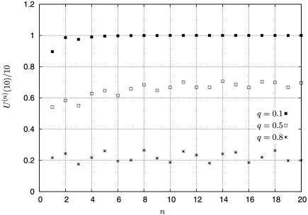
Figure 4: We consider an HCP with $d^{(n)}=2^{n-1}$ (the relevant choice to describe East model) with initial law specified in Proposition B.1 and parameter $q:=1-p=0.1,0.5,0.8$. In the first case the limit (17) exists with $c_{0}=1$. Instead, for $q=0.5,0.8$ as proven in Proposition B.1 the limit (17) does not exists. We plot here $U^{(n)}(x)/x$ for $x=10$ as a function of $n$. The data indicate clearly that for $p=0.1$ $U^{(n)}(10)/10$ converges to $1$ as we have proven [see Theorem 2.19 and especially the comment below formula (93)]. Instead of the other two choices of the parameters, $U^{(n)}(10)/10$ has an oscillating behavior which strongly indicates the nonexistence of the limit for $U^{(n)}(x)$, hence for $g^{(n)}(s)$. We have checked that an analogous behavior occurs for different choices of $x$. Note that if we were instead considering for the same initial distribution but a different choice of $d^{(n)}$ (satisfying the basic hypothesis $d^{(n)}\to\infty$ for $n\to\infty$) we would get the same behavior. Indeed if we consider for example the choice relevant for the Paste-all model, $d^{(n)}=n$, then the plot of $U^{(n)}(10)/10$ would exactly be the same as above but with $n$ replaced by $\log_{2}(n)$ in the $x$-axis (and in this case our data would cover $2^{20}$ epochs).

strongly suggest that in this case the measure $\mu^{(n)}$ does not have a well-defined limiting behavior as $n\to\infty$.

Proposition B.1

Let $G$ be a geometric random variable with parameter $p=1-e^{-\lambda}$, $\lambda\in(0,1)$. Define $X=e^{G}$ and $g(s)=\mathbb{E}(e^{-sX})$, $s\geq 0$. Then, $\lim_{s\to 0}\frac{sg^{\prime}(s)}{1-g(s)}$ does not exist. More precisely, for any $\alpha\in[0,1)$ and any $n\in\mathbb{N}$, set $s_{n}=e^{-n-\alpha}$. Then $\lim_{n\to\infty}\frac{s_{n}g^{\prime}(s_{n})}{1-g(s_{n})}=:L_{\alpha}$ exists, and ${\alpha}\rightarrow L_{\alpha}$ is a nonconstant function.

Note that the constraint ${\lambda}\in(0,1)$ is equivalent to the fact that $X$ has infinite mean. Proof of Proposition B.1 Fix $\alpha\in[0,1)$ and set $s_{n}=e^{-n-\alpha}$. Since $\mathbb{P}(G=k)=p(1-p)^{k-1}$ for $k\geq 1$, we have $\bar{F}(x)=\mathbb{P}(X\geq x)=e^{-\lambda\lceil\ln x\rceil+\lambda}=x^{-\lambda}e^{\lambda\{\ln x\}}$ where $\lceil z\rceil=z+1-\{z\}$ is the ceiling function of $z$ (i.e., the smallest integer greater than or equal to $z$), and $\{z\}\in(0,1]$ is the fractional part of $z$. Note that $\bar{F}(e)=1$.

Then, using an integration by parts and the change of variables $u=sx$, we have

$$-g^{\prime}(s) = \mathbb{E}(Xe^{-sX})=-\int_{[e,\infty)}xe^{-sx}\,d\bar{F}(x)$$

$$= e^{1-se}+\int_{[e,\infty)}(1-sx)e^{-sx}\bar{F}(x)\,dx$$

$$= e^{1-se}+\frac{1}{s}\int_{[es,\infty)}(1-u)e^{-u}\bar{F}\biggl{(}\frac{u}{s}\biggr{)}\,du$$

$$= e^{1-se}+s^{\lambda-1}\int_{[es,\infty)}(1-u)u^{-\lambda}e^{-u}e^{\lambda\{\ln u-\ln s\}}\,du.$$

Similarly

$$1-g(s)=1+\int_{[e,\infty)}e^{-sx}\,d\bar{F}(x)=1-e^{-se}+s^{\lambda}\int_{[es,\infty)}u^{-\lambda}e^{-u}e^{\lambda\{\ln u-\ln s\}}\,du.$$

Since $\{\ln u-\ln s_{n}\}=\{\ln u+\alpha\}$ for any $n$, it follows that [recall that $\lambda\in(0,1)$]

$$\lim_{n\to\infty}\frac{-s_{n}g^{\prime}(s_{n})}{1-g(s_{n})} = \lim_{n\to\infty}\frac{s_{n}e^{1-s_{n}e}+s_{n}^{\lambda}\int_{[es_{n},\infty)}(1-u)u^{-\lambda}e^{-u}e^{\lambda\{\ln u+\alpha\}}\,du}{1-e^{-s_{n}e}+s_{n}^{\lambda}\int_{[es_{n},\infty)}u^{-\lambda}e^{-u}e^{\lambda\{\ln u+\alpha\}}\,du}$$

$$= \frac{\int_{(0,\infty)}(1-u)u^{-\lambda}e^{-u}e^{\lambda\{\ln u+\alpha\}}\,du}{\int_{(0,\infty)}u^{-\lambda}e^{-u}e^{\lambda\{\ln u+\alpha\}}\,du}=:L_{\alpha}.$$

Suppose $L_{\alpha}$ to be equal to $1-C$ for all ${\alpha}$. Then, by the change of variable $v=u/{\beta}$ where ${\beta}=e^{-{\alpha}}$, we can write

$$1-L_{\alpha} = \frac{{\beta}\int_{0}^{\infty}v^{-{\lambda}+1}e^{-{\beta}{v}}e^{{\lambda}\{\ln v\}}\,dv}{\int_{0}^{\infty}v^{-{\lambda}}e^{-{\beta}{v}}e^{{\lambda}\{\ln v\}}\,dv}$$

$$= \frac{(B+1)\int_{0}^{\infty}v^{-{\lambda}+1}e^{-v}e^{-Bv}e^{{\lambda}\{\ln v\}}\,dv}{\int_{0}^{\infty}v^{-{\lambda}}e^{-Bv}e^{-v}e^{{\lambda}\{\ln v\}}\,dv}=C,$$

where $B={\beta}-1$. Consider now the functions $f$ and $g$ on ${\mathbb{D}}=\{z\in{\mathbb{C}}\dvtx|z|<1\}$ defined as

$$f(z) = \int_{0}^{\infty}v^{-{\lambda}+1}e^{-v}e^{-zv}e^{{\lambda}\{\ln v\}}\,dv,$$

$$g(z) = \int_{0}^{\infty}v^{-{\lambda}}e^{-zv}e^{-v}e^{{\lambda}\{\ln v\}}\,dv.$$

By Fubini’s theorem and the series expansion of the exponential function, one gets that $f$ and $g$ are holomorphic functions on ${\mathbb{D}}$. Hence, the same holds for the function $H(z)=(1+z)f(z)-Cg(z)$. Due to the last identity in (B) we get that $H$ is zero on a subinterval of the real line. Due to a theorem of complex analysis, the zeros of a nonconstant holomorphic function are isolated points. As a byproduct, we get that $H(z)=0$ for all $z\in{\mathbb{D}}$.

Writing the power expansion of $H(z)$ around $z=0$ and using that $H\equiv 0$, we get

$$\int_{0}^{\infty}v^{-{\lambda}+1+n}e^{-v}e^{{\lambda}\{\ln v\}}\,dv=(C-1)\int_{0}^{\infty}v^{-{\lambda}+n}e^{-v}e^{{\lambda}\{\ln v\}}\,dv\qquad\forall n\geq 0.$$

Note that it must be $C>1$. By iteration we get

$$\int_{0}^{\infty}v^{-{\lambda}+n}e^{-v}e^{{\lambda}\{\ln v\}}\,dv\leq(C-1)^{n},\qquad n\geq 0.$$ (118)

On the other hand the above left-hand side is larger than $\Gamma(n+1-{\lambda}):=\int_{0}^{\infty}v^{-{\lambda}+n}e^{-v}\,dv$. Iterating the identity $\Gamma(z+1)=z\Gamma(z)$ we get that

$$\Gamma(n+1-{\lambda})=(n-{\lambda})(n-{\lambda}-1)\cdots(1-{\lambda})\Gamma(1-{\lambda}),$$

which leads to a contradiction with (118).

Appendix C ${\mathbb{Z}}$-stationary SPPs

${\mathbb{Z}}$-stationary SPPs and stationary SPPs have many common features. In this Appendix we point out some properties of ${\mathbb{Z}}$-stationary SPPs, whose proof (only sketched here) follows by suitably adapting the arguments used in the continuous case.

Let us suppose that ${\mathcal{Q}}$ is the law of a ${\mathbb{Z}}$-stationary SPP, nonempty a.s. We derive here some identities relating ${\mathcal{Q}}$ to the conditional probability measure ${\mathcal{Q}}_{0}:={\mathcal{Q}}(\cdot|0\in\xi)$. These identities are similar to the ones relating the law of a stationary SPP to its Palm distribution DV , FKAS . Since all random sets are included in ${\mathbb{Z}}$ it is more natural to work with the subspaces of ${\mathcal{N}}$ defined as

$${\mathcal{N}}^{{\mathbb{Z}}} = \{\xi\in{\mathcal{N}}\dvtx\xi\subset{\mathbb{Z}}\},$$ (119)

$${\mathcal{N}}^{{\mathbb{Z}}}_{0} = \{\xi\in{\mathcal{N}}^{\mathbb{Z}}\dvtx 0\in\xi\}.$$ (120)

Moreover, we prefer to write ${\tau}_{x}\xi$ instead of $\xi-x$.

Similarly to (4) we get a simple relation characterizing ${\mathcal{Q}}$ by means of ${\mathcal{Q}}_{0}$:

Lemma C.1

Given a nonnegative measurable function $f$ on ${\mathcal{N}}^{\mathbb{Z}}$ it holds

$$\int{\mathcal{Q}}(d\xi)f(\xi)={\mathcal{Q}}(0\in\xi)\int{\mathcal{Q}}_{0}(d\xi)\sum_{x=0}^{x_{1}(\xi)-1}f({\tau}_{x}\xi).$$ (121)

From the ${\mathbb{Z}}$-stationarity of ${\mathcal{Q}}$ it is simple to derive for all measurable functions $g\dvtx{\mathcal{N}}^{{\mathbb{Z}}}_{0}\to[0,\infty)$ and $t\in{\mathbb{N}}_{+}$ that

$$\int{\mathcal{Q}}_{0}(d\xi)g(\xi)=\frac{1}{t{\mathcal{Q}}(0\in\xi)}\int{\mathcal{Q}}(d\xi)\sum_{y\in\xi\cap(0,t]}g({\tau}_{y}\xi).$$ (122)

Given a measurable map $v\dvtx{\mathbb{Z}}\times{\mathcal{N}}^{\mathbb{Z}}_{0}\to[0,\infty)$, setting $g(\xi)=\sum_{x\in{\mathbb{Z}}}v(x,\xi)$ in the above identity, we get

$$\qquad\sum_{x\in{\mathbb{Z}}}\int{\mathcal{Q}}_{0}(d\xi)v(x,\xi)=\frac{1}{t{\mathcal{Q}}(0\in\xi)}\int{\mathcal{Q}}(d\xi)\sum_{x\in{\mathbb{Z}}}\sum_{y\in\xi\cap(0,t]}v(x,{\tau}_{y}\xi).$$ (123)

Reasoning as in the proof of (1.2.10) in FKAS , for any measurable function $w\dvtx{\mathbb{Z}}\times{\mathbb{Z}}\times{\mathcal{N}}^{\mathbb{Z}}\to[0,\infty)$ we get

$$\sum_{x\in{\mathbb{Z}}}\sum_{y\in{\mathbb{Z}}}\int{\mathcal{Q}}(d\xi)w(x,y,{\tau}_{y}\xi)\mathbh{1}(y\in\xi)$$

(124)

$$\qquad=\sum_{x\in{\mathbb{Z}}}\sum_{y\in{\mathbb{Z}}}\int{\mathcal{Q}}(d\xi)w(y,x,{\tau}_{y}\xi)\mathbh{1}(y\in\xi).$$

Combining (123) with (C) where $w(x,y,\xi)=v(x,\xi)\mathbh{1}(y\in(0,t])/t$ we get

$$\quad\sum_{x\in{\mathbb{Z}}}\int{\mathcal{Q}}_{0}(d\xi)v(x,\xi)=\frac{1}{{\mathcal{Q}}(0\in\xi)}\sum_{x\in{\mathbb{Z}}}\int{\mathcal{Q}}(d\xi)v(x,{\tau}_{x}\xi)\mathbh{1}(x\in\xi).$$ (125)

At this point, we take

$$v(x,\xi):=\mathbh{1}\bigl{(}x=x_{0}({\tau}_{-x}\xi)\bigr{)}f({\tau}_{-x}\xi)$$

[if $\xi=\varnothing$ we set $v(x,\xi)=0$]. Note that $v(x,{\tau}_{x}\xi)=\mathbh{1}(x=x_{0}(\xi))f(\xi)$, thus implying together with (125) that

$$\int{\mathcal{Q}}(d\xi)f(\xi) = \sum_{x\in{\mathbb{Z}}}\int{\mathcal{Q}}(d\xi)v(x,{\tau}_{x}\xi)\mathbh{1}(x\in\xi)$$

$$= {\mathcal{Q}}(0\in\xi)\sum_{x\in{\mathbb{Z}}}\int{\mathcal{Q}}_{0}(d\xi)v(x,\xi).$$

In order to understand the last integral, take $\xi\in{\mathcal{N}}^{{\mathbb{Z}}}_{0}$. Then $x=x_{0}({\tau}_{-x}\xi)$ if and only if $0\leq-x<x_{1}(\xi)$. Therefore, changing at the end $x$ into $-x$, we get

$$\qquad\sum_{x\in{\mathbb{Z}}}v(x,\xi)=\mathop{\sum_{x\in{\mathbb{Z}}:}}_{0\leq-x<x_{1}(\xi)}f({\tau}_{-x}\xi)=\sum_{x=0}^{x_{1}(\xi)-1}f({\tau}_{x}\xi)\qquad\forall\xi\in{\mathcal{N}}^{{\mathbb{Z}}}_{0}.$$ (127)

Combining (C) and (127) we get the thesis.

Taking $f=1$ in (121) we deduce that $x_{1}(\xi)$ must have finite mean w.r.t. ${\mathcal{Q}}_{0}$. In particular, if ${\mathcal{Q}}_{0}$ is the law of the renewal SPP on ${\mathbb{Z}}$ containing the origin and with domain length $\mu$ [i.e., ${\mathcal{Q}}_{0}$ is the law of $\operatorname{Ren}_{0}(\mu)$], then $\mu$ must have finite mean. On the other hand, given $\mu$ probability measure on ${\mathbb{N}}_{+}$ with finite mean, identity (121) uniquely determines the probability measure ${\mathcal{Q}}$ if ${\mathcal{Q}}_{0}$ is defined as the law of $\operatorname{Ren}(\mu\mid 0)$. One can then prove that the so-defined ${\mathcal{Q}}$ is the law of a ${\mathbb{Z}}$-stationary SPP and that ${\mathcal{Q}}_{0}={\mathcal{Q}}(\cdot|0\in\xi)$. Finally, as in the continuous case, relation (121) allows us to derive a simple description of ${\mathbb{Z}}$-stationary renewal SPPs similar to the one mentioned after Definition 2.7. We leave the details to the interested reader.

Appendix D Exchangeable SPPs

We endow the space ${\Omega}=(0,\infty)^{{\mathbb{N}}_{+}}$ of sequences of positive numbers with the product topology, and we denote by ${\mathcal{B}}$ its Borel $\sigma$-field. We write a generic element of ${\Omega}$ as ${\omega}=({\omega}_{n}\dvtx n\in{\mathbb{N}}_{+})$. Let ${\mathcal{E}}_{n}$ be the $\sigma$-subfield generated by the events that are invariant under permutations of ${\mathbb{Z}}$ fixing all points $x\in{\mathbb{N}}_{+}$ with $x>n$. Let ${\mathcal{E}}:=\bigcap_{n=1}^{\infty}{\mathcal{E}}_{n}$ be the exchangeable $\sigma$-field. Since ${\Omega}$ is a standard Borel set, given a probability measure $Q$ on ${\Omega}$ there exists a regular conditional probability associated to ${\mathcal{E}}$, that is, a measurable map $\rho_{Q}\dvtx{\Omega}\times{\mathcal{B}}\to[0,1]$ satisfying the following properties:

for each $A\in{\mathcal{B}}$, $\rho_{Q}(\cdot,A)$ is a version of $P(A|{\mathcal{E}})$;

for $Q$-a.e. ${\omega}\in{\Omega}$, $\rho_{Q}({\omega},\cdot)$ is a probability measure on $({\Omega},{\mathcal{B}})$.

Due to de Finetti’s theorem, if $Q$ is an exchangeable probability measure on ${\Omega}$, then for $Q$-a.e. ${\omega}$ the measure $\rho_{Q}({\omega},\cdot)$ is a product probability measure on ${\Omega}$. The inverse implication is trivially true; hence de Finetti’s theorem provides a characterization of the exchangeable probability measures on ${\Omega}$.

Suppose that ${\mathcal{Q}}$ is a left-bounded exchangeable SPP containing the origin (see Definition 2.9). By definition, ${\mathcal{Q}}$ has support on the subspace $\Xi\subset{\mathcal{N}}$ given by the configurations $\xi\in{\mathcal{N}}$ empty on $(-\infty,0)$, containing the origin and given by a sequence of points $x_{k}(\xi)$, $k\in{\mathbb{N}}$, diverging to $+\infty$. We can define the measurable injective map $\Psi\dvtx\Xi\to{\Omega}$, with $\Psi(\xi)={\omega}$ and ${\omega}_{n}=x_{n}(\xi)-x_{n-1}(\xi)$. We call $Q$ the measure ${\mathcal{Q}}\circ\Psi^{-1}$. Trivially, $Q$ is an exchangeable measure on ${\Omega}$; hence we can apply de Finetti’s theorem and get $Q(A)=\int_{\Omega}Q(d{\omega})\rho_{Q}({\omega},A)$ for all $A\in{\mathcal{B}}$, where $\rho_{Q}({\omega},\cdot)$ is a product probability measure. Since trivially $\rho_{Q}({\omega},\cdot)$ has support on $\Psi(\Xi)$, the pull-back of $\rho_{Q}({\omega},\cdot)$ is a well-defined probability measure on $\Xi$ corresponding to the law of $\operatorname{Ren}({\delta}_{0},\mu_{\omega})$. As byproduct, we get

$${\mathcal{Q}}({\mathcal{A}})=\int_{\Omega}Q(d{\omega})\operatorname{Ren}({\delta}_{0},\mu_{\omega})[{\mathcal{A}}],\qquad{\mathcal{A}}\subset{\mathcal{N}}\mbox{ measurable}.$$ (128)

The above decomposition allows us to extend our results stated in Section 2 to right exchangeable SPPs containing the origin. We give only some comments, leaving the details to the interested reader. Consider, for example, the HCP starting from ${\mathcal{Q}}$, that is, $\xi^{(1)}(0)$ has law ${\mathcal{Q}}$. By applying inductively Theorem 2.13 we get that, given $n\geq 1$ and $t\in[0,\infty]$, the law of $\xi^{(n)}(t)$ conditioned to the fact that $0\in\xi^{(n)}(t)$ has the integral representation

$$\int_{{\Omega}}Q(d{\omega})\operatorname{Ren}\bigl{(}{\delta}_{0},[\mu_{\omega}]^{(n)}_{t}\bigr{)}$$

for a suitable probability measure $[\mu_{\omega}]^{(n)}_{t}$ on $(0,\infty)$.

In particular, if each $\mu_{\omega}$ satisfies the limit (17) for some constant $c_{0}({\omega})$, we get the following: fixed $k\geq 1$, the rescaled random variable $[x_{k}^{(n)}(0)-x_{k-1}^{(n)}(0)]/d_{\min}^{(n)}$, defined for the HCP starting with law ${\mathcal{Q}}$ and conditioned to the event $\{0\in\xi^{(n)}(0)\}$, weakly converges to a random variable whose Laplace transform $g^{(\infty)}$ is given by

$$g^{(\infty)}(s)=\int_{{\Omega}}Q(d{\omega})g^{\infty}_{c_{0}({\omega})}(s),$$

where $g^{\infty}_{(c_{0})}$ has been defined in (18). Note that new limit laws emerge in this way.

Let us now pass to stationary exchangeable SPPs. One can formulate de Finetti’s theorem also for exchangeable laws on the space ${\Omega}^{\prime}=(0,\infty)^{\mathbb{Z}}$ of two-sided sequences of positive numbers. At the end we get that a stationary SPP, nonempty a.s. and with finite intensity, is exchangeable if and only if its Palm distribution ${\mathcal{Q}}_{0}$ satisfies

$${\mathcal{Q}}_{0}({\mathcal{A}})=\int_{{\Omega}^{\prime}}Q(d{\omega})\operatorname{Ren}_{0}(\mu_{\omega})[{\mathcal{A}}],\qquad{\mathcal{A}}\subset{\mathcal{N}}\mbox{ measurable},$$ (129)

where (i) $\mu_{\omega}$ is a probability measure on $(0,\infty)$; (ii) for any ${\mathcal{A}}\subset{\mathcal{N}}$ measurable the map ${\Omega}^{\prime}\ni{\omega}\to\operatorname{Ren}_{0}(\mu_{\omega})[{\mathcal{A}}]$ is measurable (thus implying that the map ${\omega}\to\mu_{\omega}$ is measurable); (iii) $Q$ is the image of the law ${\mathcal{Q}}$ of the SPP under the map ${\mathcal{N}}^{\infty}_{0}\to(0,\infty)^{\mathbb{Z}}$, mapping $\xi$ in $(x_{k}(\xi)-x_{k-1}(\xi)\dvtx k\in{\mathbb{Z}})$ [recall (3)].

Using (129) and (4) we conclude that

$${\mathcal{Q}}({\mathcal{A}})=\int_{{\Omega}^{\prime}}Q(d{\omega})\operatorname{Ren}(\mu_{\omega})[{\mathcal{A}}],\qquad{\mathcal{A}}\subset{\mathcal{N}}\mbox{ measurable}.$$ (130)

The above decomposition of ${\mathcal{Q}}$ allows us to extend our limit theorems to the HCP starting with law ${\mathcal{Q}}$, that is, from a stationary exchangeable SPPs. In particular, $\xi^{(n)}(t)$ will be a stationary exchangeable SPP for all $n\geq 1$ and all $t\in[0,\infty]$. In addition, for $k\not=1$, as $n\to\infty$ the rescaled random variable $[x_{k}^{(n)}(0)-x_{k-1}^{(n)}(0)]/d_{\min}^{(n)}$ weakly converges to the random variable $Z^{(\infty)}_{1}$ introduced in Theorem 2.19.

Appendix E A combinatorial lemma on exchangeable probability measures

The next combinatorial lemma has been used in Section 3.

Lemma E.1

Let $m_{k}$ be an exchangeable probability measure on $S^{k}$, $S=(0,\infty)$; that is, $m_{k}$ is left invariant by any permutation of the coordinates $(s_{1},\ldots,s_{k})\in S^{k}$. Call $m$ the marginal of $m_{k}$ along a coordinate (it does not depend on the coordinate). Then, for any bounded function $f\dvtx S\to\mathbb{R}$, and any bounded function $g\dvtx S\to(0,\infty)$, it holds

$$\mbox{{(a)}}\quad\mathbb{E}_{m_{k}}\Biggl{(}\frac{g(s_{1})}{g(s_{1})+\cdots+g(s_{k})}\prod_{i=2}^{k-1}\frac{g(s_{i})}{\sum_{j=i}^{k-1}g(s_{j})}\prod_{i=1}^{k}f(s_{i})\Biggr{)}=\frac{\mathbb{E}_{m}(f)^{k}}{k\cdot(k-2)!},$$

$$\mbox{{(b)}}\quad\hskip 130.3pt\mathbb{E}_{m_{k}}\Biggl{(}\prod_{i=1}^{k}\frac{g(s_{i})f(s_{i})}{\sum_{j=i}^{k}g(s_{j})}\Biggr{)}=\frac{\mathbb{E}_{m}(f)^{k}}{k!}.$$

We will give only the proof of point (a) which is a bit harder. The proof of point (b) follows essentially the same lines; details are left to the reader.

Since the law $m_{k}$ is left invariant by any permutations of the coordinates $(s_{1},\ldots,s_{k})\in S^{k}$, we have

$$\mathbb{E}_{m_{k}}\Biggl{(}\frac{g(s_{1})}{g(s_{1})+\cdots+g(s_{k})}\prod_{i=2}^{k-1}\frac{g(s_{i})}{\sum_{j=i}^{k-1}g(s_{j})}\prod_{i=1}^{k}f(s_{i})\Biggr{)}$$

$$\qquad=\frac{1}{k!}\sum_{\sigma\in\mathcal{S}_{k}}\mathbb{E}_{m_{k}}\Biggl{(}\frac{g(s_{\sigma(1)})}{g(s_{\sigma(1)})+\cdots+g(s_{\sigma(k)})}\prod_{i=2}^{k-1}\frac{g(s_{\sigma(i)})}{\sum_{j=i}^{k-1}g(s_{\sigma(j)})}\prod_{i=1}^{k}f\bigl{(}s_{\sigma(i)}\bigr{)}\Biggr{)}$$

$$\qquad=\frac{1}{k!}\mathbb{E}_{m_{k}}\Biggl{(}f(s_{1})\cdots f(s_{k})\sum_{\sigma\in\mathcal{S}_{k}}\frac{g(s_{\sigma(1)})}{g(s_{1})+\cdots+g(s_{k})}\prod_{i=2}^{k-1}\frac{g(s_{\sigma(i)})}{\sum_{j=i}^{k-1}g(s_{\sigma(j)})}\Biggr{)},$$

where $\mathcal{S}_{k}$ stands for the symmetric group of $\{1,\ldots,k\}$. Hence the result will follow from the identity

$$\sum_{\sigma\in\mathcal{S}_{k}}\frac{g(s_{\sigma(1)})}{g(s_{1})+\cdots+g(s_{k})}\prod_{i=2}^{k-1}\frac{g(s_{\sigma(i)})}{\sum_{j=i}^{k-1}g(s_{\sigma(j)})}=k-1$$ (131)

and the product structure of $m_{k}$. Now we prove (131). Divide the sum in (131) depending on the value of $\sigma(1)$ and $\sigma(k)$

$$\mbox{l.h.s. of (\ref{eqidentity})}=\sum_{i_{1}=1}^{k}\frac{g(s_{i_{1}})}{g(s_{1})+\cdots+g(s_{k})}\mathop{\sum_{i_{k}=1}}_{i_{k}\neq i_{1}}^{k}\mathop{\mathop{\sum_{\sigma\in\mathcal{S}_{k}:}}_{\sigma(1)=i_{1}}}_{\sigma(k)=i_{k}}\prod_{i=2}^{k-1}\frac{g(s_{\sigma(i)})}{\sum_{j=i}^{k-1}g(s_{\sigma(j)})}.$$

The thesis will follow from the fact that, for any $i_{1},i_{k}$, the last sum in the latter is equal to 1. Equivalently, we need to prove that, for any $n$,

$$\sum_{\sigma\in\mathcal{S}_{n}}\prod_{i=1}^{n}\frac{g(s_{\sigma(i)})}{\sum_{j=i}^{n}g(s_{\sigma(j)})}=1.$$ (132)

This is done by induction. Indeed, the thesis is trivial for $n=1$. Assume that (132) holds at rank $n-1$. Then,

$$\sum_{\sigma\in\mathcal{S}_{n}}\prod_{i=1}^{n}\frac{g(s_{\sigma(i)})}{\sum_{j=i}^{n}g(s_{\sigma(j)})}$$

$$\qquad=\sum_{i_{1}=1}^{n}\mathop{\sum_{\sigma\in\mathcal{S}_{n}:}}_{\sigma(1)=i_{1}}\prod_{i=1}^{n}\frac{g(s_{\sigma(i)})}{\sum_{j=i}^{n}g(s_{\sigma(j)})}$$

$$\qquad=\sum_{i_{1}=1}^{n}\frac{g(s_{i_{1}})}{g(s_{1})+g(s_{2})+\cdots+g(s_{n})}\mathop{\sum_{\sigma\in\mathcal{S}_{n}:}}_{\sigma(1)=i_{1}}\prod_{i=2}^{n}\frac{g(s_{\sigma(i)})}{\sum_{j=i}^{n}g(s_{\sigma(j)})}.$$

Note that, by the induction hypothesis, the second sum is equal to $1$ (for any $i_{1}$). Hence,

$$\sum_{\sigma\in\mathcal{S}_{n}}\prod_{i=1}^{n}\frac{g(s_{\sigma(i)})}{\sum_{j=i}^{n}g(s_{\sigma(j)})}=\sum_{i_{1}=1}^{n}\frac{g(s_{i_{1}})}{g(s_{1})+g(s_{2})+\cdots+g(s_{n})}=1.$$

This ends the proof of (132) and thus of point (a). As already mentioned the proof of point (b) is easier [only (132) has to be used]; details are left to the reader.

References

- (1) {barticle}[mr] \bauthor\bsnmAldous, \bfnmDavid J.\binitsD. J. (\byear1999). \btitleDeterministic and stochastic models for coalescence (aggregation and coagulation): A review of the mean-field theory for probabilists. \bjournalBernoulli \bvolume5 \bpages3–48. \biddoi=10.2307/3318611, issn=1350-7265, mr=1673235 \endbibitem
- (2) {barticle}[mr] \bauthor\bsnmBertoin, \bfnmJean\binitsJ. (\byear2001). \btitleEternal additive coalescents and certain bridges with exchangeable increments. \bjournalAnn. Probab. \bvolume29 \bpages344–360. \biddoi=10.1214/aop/1008956333, issn=0091-1798, mr=1825153 \endbibitem
- (3) {bbook}[mr] \bauthor\bsnmBertoin, \bfnmJean\binitsJ. (\byear2006). \btitleRandom Fragmentation and Coagulation Processes. \bseriesCambridge Studies in Advanced Mathematics \bvolume102. \bpublisherCambridge Univ. Press, \baddressCambridge. \biddoi=10.1017/CBO9780511617768, mr=2253162 \endbibitem
- (4) {bbook}[mr] \bauthor\bsnmBillingsley, \bfnmPatrick\binitsP. (\byear1968). \btitleConvergence of Probability Measures. \bpublisherWiley, \baddressNew York. \bidmr=0233396 \endbibitem
- (5) {barticle}[auto:STB—2011-03-03—12:04:44] \bauthor\bsnmBray, \bfnmA. J.\binitsA. J., \bauthor\bsnmDerrida, \bfnmB.\binitsB. and \bauthor\bsnmGordrèche, \bfnmC.\binitsC. (\byear1994). \btitleNon-trivial algebraic decay in a soluble model of coarsening. \bjournalEurophys. Lett. \bvolume27 \bpages175–180. \endbibitem
- (6) {bbook}[mr] \bauthor\bsnmDaley, \bfnmD. J.\binitsD. J. and \bauthor\bsnmVere-Jones, \bfnmD.\binitsD. (\byear1988). \btitleAn Introduction to the Theory of Point Processes. \bpublisherSpringer, \baddressNew York. \bidmr=0950166 \endbibitem
- (7) {barticle}[auto:STB—2011-03-03—12:04:44] \bauthor\bsnmDerrida, \bfnmB.\binitsB., \bauthor\bsnmBray, \bfnmA. J.\binitsA. J. and \bauthor\bsnmGodrèche, \bfnmC.\binitsC. (\byear1994). \btitleNon-trivial exponents in the zero temperature dynamics of the 1d Ising and Potts model. \bjournalJ. Phys. A \bvolume27 \bpagesL357–L361. \endbibitem
- (8) {barticle}[auto:STB—2011-03-03—12:04:44] \bauthor\bsnmDerrida, \bfnmB.\binitsB., \bauthor\bsnmGodrèche, \bfnmC.\binitsC. and \bauthor\bsnmYekutieli, \bfnmI.\binitsI. (\byear1990). \btitleStable distributions of growing and coalescing droplets. \bjournalEurophys. Lett. \bvolume12 \bpages385–390. \endbibitem
- (9) {barticle}[auto:STB—2011-03-03—12:04:44] \bauthor\bsnmDerrida, \bfnmB.\binitsB., \bauthor\bsnmGodrèche, \bfnmC.\binitsC. and \bauthor\bsnmYekutieli, \bfnmI.\binitsI. (\byear1991). \btitleScale invariant regime in the one dimensional models of growing and coalescing droplets. \bjournalPhys. Rev. A \bvolume44 \bpages6241–6251. \endbibitem
- (10) {bbook}[mr] \bauthor\bsnmDurrett, \bfnmRichard\binitsR. (\byear1996). \btitleProbability: Theory and Examples, \bedition2nd ed. \bpublisherDuxbury Press, \baddressBelmont, CA. \bidmr=1609153 \endbibitem
- (11) {barticle}[auto:STB—2011-03-03—12:04:44] \bauthor\bsnmEisinger, \bfnmS.\binitsS. and \bauthor\bsnmJackle, \bfnmJ.\binitsJ. (\byear1991). \btitleA hierarchically constrained kinetic ising model. \bjournalZ. Phys. B \bvolume84 \bpages115–124. \endbibitem
- (12) {bmisc}[auto:STB—2011-03-03—12:04:44] \bauthor\bsnmFaggionato, \bfnmA.\binitsA., \bauthor\bsnmMartinelli, \bfnmF.\binitsF., \bauthor\bsnmRoberto, \bfnmC.\binitsC. and \bauthor\bsnmToninelli, \bfnmC.\binitsC. (\byear2010). \bhowpublishedAging through hierarchical coalescence in the East model. Preprint. Available at arXiv:1012.4912. \endbibitem
- (13) {bmisc}[auto:STB—2011-03-03—12:04:44] \bauthor\bsnmFaggionato, \bfnmA.\binitsA., \bauthor\bsnmMartinelli, \bfnmF.\binitsF., \bauthor\bsnmRoberto, \bfnmC.\binitsC. and \bauthor\bsnmToninelli, \bfnmC.\binitsC. (\byear2011). \bhowpublishedUnpublished manuscript. \endbibitem
- (14) {bbook}[mr] \bauthor\bsnmFeller, \bfnmWilliam\binitsW. (\byear1971). \btitleAn Introduction to Probability Theory and Its Applications. Vol. II, \bedition2nd ed. \bpublisherWiley, \baddressNew York. \bidmr=0270403 \endbibitem
- (15) {bbook}[mr] \bauthor\bsnmFranken, \bfnmPeter\binitsP., \bauthor\bsnmKönig, \bfnmDieter\binitsD., \bauthor\bsnmArndt, \bfnmUrsula\binitsU. and \bauthor\bsnmSchmidt, \bfnmVolker\binitsV. (\byear1982). \btitleQueues and Point Processes. \bpublisherWiley, \baddressChichester. \bidmr=0691670 \endbibitem
- (16) {barticle}[mr] \bauthor\bsnmGallay, \bfnmT.\binitsT. and \bauthor\bsnmMielke, \bfnmA.\binitsA. (\byear2003). \btitleConvergence results for a coarsening model using global linearization. \bjournalJ. Nonlinear Sci. \bvolume13 \bpages311–346. \biddoi=10.1007/s00332-002-0543-8, issn=0938-8974, mr=1982018 \endbibitem
- (17) {bbook}[mr] \bauthor\bsnmKallenberg, \bfnmOlav\binitsO. (\byear2005). \btitleProbabilistic Symmetries and Invariance Principles. \bpublisherSpringer, \baddressNew York. \bidmr=2161313 \endbibitem
- (18) {barticle}[mr] \bauthor\bsnmLimic, \bfnmVlada\binitsV. and \bauthor\bsnmSturm, \bfnmAnja\binitsA. (\byear2006). \btitleThe spatial -coalescent. \bjournalElectron. J. Probab. \bvolume11 \bpages363–393 (electronic). \bidissn=1083-6489, mr=2223040 \endbibitem
- (19) {bbook}[mr] \bauthor\bsnmMatthes, \bfnmKlaus\binitsK., \bauthor\bsnmKerstan, \bfnmJohannes\binitsJ. and \bauthor\bsnmMecke, \bfnmJoseph\binitsJ. (\byear1978). \btitleInfinitely Divisible Point Processes. \bpublisherWiley, \baddressNew York. \bidmr=0517931 \endbibitem
- (20) {bincollection}[mr] \bauthor\bsnmPego, \bfnmRobert L.\binitsR. L. (\byear2007). \btitleLectures on dynamics in models of coarsening and coagulation. In \bbooktitleDynamics in Models of Coarsening, Coagulation, Condensation and Quantization. \bseriesLect. Notes Ser. Inst. Math. Sci. Natl. Univ. Singap. \bvolume9 \bpages1–61. \bpublisherWorld Scientific, \baddressHackensack, NJ. \biddoi=10.1142/9789812770226_0001, mr=2395779 \endbibitem
- (21) {bbook}[auto:STB—2011-03-03—12:04:44] \beditor\bsnmPrivman, \bfnmV.\binitsV., ed. (\byear1997). \btitleNon Equilibrium Statistical Mechanics in One Dimension. \bpublisherCambridge Univ. Press, \baddressNew York. \endbibitem
- (22) {barticle}[auto:STB—2011-03-03—12:04:44] \bauthor\bsnmSollich, \bfnmP.\binitsP. and \bauthor\bsnmEvans, \bfnmM. R.\binitsM. R. (\byear2003). \btitleGlassy dynamics in the asymmetrically constrained kinetic Ising chain. \bjournalPhys. Rev. E \bvolume68 \bpages031504. \endbibitem