Unstable-particles pair production in modified perturbation theory in NNLO

Abstract:

We consider pair production and decay of fundamental unstable particles in the framework of a modified perturbation theory (MPT), which treats resonant contributions of unstable particles in the sense of distributions. The cross-section of the process is calculated within the NNLO of the MPT in a model that admits exact solution. Universal massless-particles contributions are taken into consideration. The calculations are carried out by means of FORTRAN code with double precision, which ensures per mille accuracy of computations. A comparison of the outcomes with the exact solution reveals an excellent convergence of the MPT series at the energies close to and above the maximum of the cross-section. Near the maximum of the cross-section the discrepancy of the NNLO approximation makes up a few per mille.

A description of processes of production and decays of fundamental unstable particles for colliders subsequent to LHC should be made generally with the NNLO accuracy. This implies that the calculations must provide gauge cancellations and unitarity, and enough high accuracy of computation of resonant contributions. The existing methods, such as the DPA successfully applied at LEP2 [1] or the complex-mass scheme (CMS) [2] intended mainly to ILC [3], provide only the NLO precision of the description. The pinch-technique method [4], another for a long time developed approach, in principle can provide the NNLO precision, but for the maintenance of the gauge cancellations it requires a lot of calculations of extra contributions that become apparent formally at the next level of the precision, which is impractical [5]. So alternative approaches are required. A modified perturbation theory (MPT) [6, 7, 8] is such an approach. Its main feature is the direct expansion of the probability instead of amplitude in powers of the coupling constant with the aid of distribution-theory methods. As the expansion is made in powers of the coupling constant and the object to be expanded is gauge invariant, the gauge cancellations in the MPT should be automatically maintained. However, the accuracy of the description remains unknown. To clear up this question numerical simulations are required. In this report I present results of the appropriate calculations and, simultaneously, do a brief introduction to the MPT method.

Actually I will discuss the case of pair production of unstable particles. The most crucial in this case are the double-resonant contributions. The corresponding total cross-section, for example in $e^{+}e^{-}$ annihilation, has the form of a convolution of the hard-scattering cross-section with the flux function,

$$\sigma(s)=\int_{s_{\mbox{\tiny min}}}^{s}\frac{\mbox{d}s^{\prime}}{s}\>\phi(s^{\prime}/s;s)\>\hat{\sigma}(s^{\prime})\,.$$ (1)

(In fact the angular distributions may be described in the MPT, as well, but I do not discuss this option below.) The hard-scattering cross-section has the form of an integral over the virtualities of unstable particles,

$$\hat{\sigma}(s)=\int\!\!\!\!\int\mbox{d}s_{1}\,\mbox{d}s_{2}\;\theta(\!\sqrt{s}-\!\sqrt{s_{1}}-\!\sqrt{s_{2}}\,)\sqrt{\lambda(s,s_{1},s_{2})}\;\Phi(s;s_{1},s_{2})\left(1\!+\!\delta_{c}\right)\,\rho(s_{1})\>\rho(s_{2})\,.$$ (2)

Here the first two multipliers in the integrand are kinematic factors, $\rho(s_{i})$ are Breit-Wigner (BW) factors, $(1\!+\!\delta_{c})$ stands for soft massless-particles contributions, and function $\Phi$ is the rest of the amplitude squared. Generally $\Phi$ corresponds to one-particle irreducible contributions, and hence $\Phi$ has no singularities on the mass-shell of unstable particles. On the contrary, the kinematic factors have singularities due to the theta function and the square root of the kinematic function $\lambda$. The BW factors if to naively expand them in powers of the coupling constant $\alpha$ generate nonintegrable singularities. Actually this constitutes a serious problem since integrals in (2) become senseless.

The singularities, nevertheless, become integrable if to expand the BW factors in the sense of distributions. In this case the expansion of a separately taken BW factor is beginning with the $\delta$-function which corresponds to the narrow-width approximation. The contributions of the naive Taylor expansion are supplied with the principal-value prescription for the poles. The nontrivial contributions are the delta-function and its derivatives with coefficients $c_{n}$, which are polynomials in $\alpha$ determined by the self-energy of the unstable particle [6]. Within the NNLO, the expansion has the form

$$\displaystyle\rho(s)\;\;\equiv\;\;\frac{M\Gamma_{0}}{\pi}\;{|s-M^{2}+\Sigma(s)|^{-2}}\;\;=$$ (3)

$$\displaystyle\quad\;\;\delta(s\!-\!M^{2})\,+\,\frac{M\Gamma_{0}}{\pi}\,PV\!\left[\,\frac{1}{(s-M^{2})^{2}}-\,\frac{2\alpha\,\mbox{Re}\Sigma_{1}(s)}{(s\!-\!M^{2})^{3}}\,\right]\;+\;\sum\limits_{n\,=\,0}^{2}c_{n}(\alpha)\,\frac{\mbox{\small($-$)}^{n}}{n!}\,\delta^{(n)}(s\!-\!M^{2})+O(\alpha^{3})\,.$$

Here $M$ is the renormalized mass, $\Gamma_{0}$ is the Born width, $\Sigma(s)$ is the self-energy of the unstable particle. Coefficients $c_{n}$ within the NNLO include 3-loop self-energy contributions and their derivatives, determined on-shell. The structure of the contributions is such that in the OMS-type schemes of the UV renormalization the real self-energy contributions enter into the coefficients either without the derivatives or with the first derivative only. This implies that the relevant real self-energy contributions are determined by the renormalization conditions. Unfortunately, the conventional OMS scheme is not convenient, since it does not maintain the gauge independence of the renormalized masses of unstable particles. So it is reasonable to proceed to the particular version of the OMS scheme, namely to the $\overline{\mbox{OMS}}$ or pole scheme [9, 10], where the renormalized masses of unstable particles by definition coincide with the real parts of the poles of the propagators and thereby coincide with the observable masses. The coefficients $c_{n}$ in this scheme are determined as follows [8]:

$$c_{0}=-\,\alpha\,\frac{I_{2}}{I_{1}}+\alpha^{2}\left[\frac{I_{2}^{2}}{I^{2}_{1}}-\frac{I_{3}}{I_{1}}-(I_{1}^{\,\prime})^{2}\right],\qquad c_{1}=0,\qquad c_{2}=-\,\alpha^{2}I^{2}_{1}\,.$$ (4)

Here $I_{k}=\mbox{Im}\,\Sigma_{k}(M^{2})$, $\Sigma=\alpha\,\Sigma_{1}+\alpha^{2}\,\Sigma_{2}+\alpha^{3}\,\Sigma_{3}$, and $I_{1}^{\,\prime}=\mbox{Im}\,\Sigma^{\,\prime}_{1}(M^{2})$. Simultaneously in the $\overline{\mbox{OMS}}$ scheme the $\mbox{Im}\,\Sigma(M^{2})$ coincides with the imaginary part of the pole of the propagator. This allows one to connect $I_{k}$ order-by-order with the width of the unstable particle via the unitarity relations $\alpha I_{1}=M\Gamma_{0}$,  $\alpha^{2}I_{2}=M\alpha\Gamma_{1}$,  and  $\alpha^{3}I_{3}=M\alpha^{2}\Gamma_{2}+\Gamma_{0}^{3}/(8M)$ [9].

In fact, expansion (3) has sense only if the weight in the integral is a regular enough function. In our case, however, the kinematic factor is not regular, and this leads to the divergence of integrals (2) after the substitution of the expansions. At first glance this closes a possibility of application of the expansions for the BW factors. Nevertheless, the kinematic factor may be analytically regularized via the substitution $[\lambda(s,s_{1},s_{2})]^{1/2}\to[\lambda(s,s_{1},s_{2})]^{\nu}$. With large enough $\lambda$ this imparts enough smoothness to the weight, and the singular integrals become integrable. Moreover, after the calculation of the integrals and removing the regularization the outcomes remain finite and the expansion remains asymptotic [8]. In principle, this salvages the applicability of the approach.

However, the singular integrals must be analytically calculated. The scheme of their calculation is as follows. At first one should proceed to dimensionless energy variables $x$, $x_{i}$ (i = 1,2) counted off from thresholds, $\sqrt{s}=2M(1+x/4)$, $\sqrt{s_{i}}=M(1+x_{i}/2)$. Formula (2) for the hard-scattering cross-section (with the analytically regularized kinematic factor) then takes the form

$$\widetilde{\sigma}(x)=\int\!\!\!\!\int\!\mbox{d}x_{1}\,\mbox{d}x_{2}\;(x\!-\!x_{1}\!-\!x_{2})_{+}^{\nu}\;\widetilde{\Phi}(x\,;x_{1},x_{2})\;\widetilde{\rho}(x_{1})\widetilde{\rho}(x_{2})\,.$$ (5)

Here $(x\!-\!x_{1}\!-\!x_{2})_{+}^{\nu}=\theta(x\!-\!x_{1}\!-\!x_{2})(x\!-\!x_{1}\!-\!x_{2})^{\nu}$ and tilde marks the dimensionless functions. (For convenience, factor $(1\!+\!\delta_{c})$ is included into the definition of the test function $\widetilde{\Phi}$.) Further, I substitute asymptotic expansions for $\widetilde{\rho}(x_{i})$ and consider at every $n_{i}$ in the product of the expansions the contributions of the $PVx_{i}^{-n_{i}}$ and $\delta^{(n_{i}-1)}(x_{i})$. Simultaneously, in each case, I represent the test function in the form of double Taylor expansion truncated at $x_{1}^{(n_{1}-1)}$ and $x_{2}^{(n_{2}-1)}$ plus a remainder,

$${\widetilde{\Phi}(x\,;x_{1},x_{2})}\;=\sum_{k_{1}=0}^{n_{1}-1}\sum_{k_{2}=0}^{n_{2}-1}\frac{x_{1}^{k_{1}}}{k_{1}!}\;\frac{x_{2}^{k_{2}}}{k_{2}!}\>\;\widetilde{\Phi}^{(k_{1},\,k_{2})}(x\,;0,0)\;+\;\Delta\widetilde{\Phi}(x\,;x_{1},x_{2})\,.$$ (6)

The higher powers of $x_{1}$ and $x_{2}$ in the Taylor expansion will zero the $\delta^{(n_{i}-1)}(x_{i})$ and cancel the $PVx_{i}^{-n_{i}}$. The remainder $\Delta\widetilde{\Phi}$ is determined as the difference between $\widetilde{\Phi}$ and the Taylor expansion. In fact $\Delta\widetilde{\Phi}$ is to be further expanded with respect to separately $x_{1}$ and $x_{2}$, but for brevity I do not consider this procedure explicitly (see details in [8]). I mention only that the final remainder produces a regular contribution to the integrand in formula (5), and the integrals of this contribution can be numerically calculated. At the same time, the contributions of the Taylor expansions are singular, and the integrals of them are analytically calculable. After the analytic integrating and putting $\nu\to 1/2$, a sum of regular and singular contributions appears with the singular contributions being products of regular factors and the power distributions of the type $x^{5/2\,-\,n}_{+}$ with integer $n$.

The convolution integral (1) of above contributions can be numerically calculated. In particular, the integral of singular power distributions may be calculated by means of the formula

$$\int\mbox{d}x\;\;x_{+}^{\nu}\,\phi(x)=\int\limits_{0}^{\infty}\mbox{d}x\;\;x^{\nu}\left\{\phi(x)-\sum_{k=0}^{N-1}\frac{x^{k}}{k!}\,\phi^{(k)}(0)\right\}\,,\vspace*{-0.2\baselineskip}$$ (7)

where $\phi$ is a weight and $N$ is a positive integer such that $-N\!-\!1<\mbox{Re}\,\nu<-N$. The test function $\widetilde{\Phi}$ at this stage is considered determined in the conventional perturbation theory.

For carrying out the above mentioned calculations rather general FORTRAN code with the double precision is written. The calculation of regular integrals in this code is fulfilled by Simpson method. Numerous indeterminate forms of the type $0/0$ that emerge in the integrand due to the difference structures are resolved through the introduction of linear patches. The patches diminish the errors that arise because of the loss of decimals near the indeterminacy points, and manifest themselves, in particular, in numerical instability. Of course, the patches generate the errors, too. However the latter errors are under control and are estimated as $\epsilon^{2}\varphi^{\prime\prime}_{0}/(3\varphi_{0})$, where $\epsilon$ is the size of the patch, $\varphi_{0}$ and $\varphi^{\prime\prime}_{0}$ is the integrand and its second derivative at the center of the patch. This estimate has sense of a relative error of the calculation of integral inside the patch. The sizes of the patches are so determined that the singular components of indeterminate forms take a constant value on the boundaries of the patches. So, for instance, in the case of an indeterminate form of the type $x^{n}/x^{n}$ the size $\epsilon$ should be so chosen that $\epsilon^{n}$ would be a constant, say, $10^{-N}$ with some fixed $N$.

Unfortunately, the errors caused by the loss of decimals near the indeterminacy points but outside of the patches, cannot be explicitly estimated. What is possible to formulate is only the dependence of these errors on the basic parameters. So, in the case of indeterminacy $[f(x)-f(0)]/x$ the appropriate error has a behavior $\sim 10^{-(D-N)}f_{0}/f^{\,\prime}_{0}$, where $D$ is the number of digits in the representation of real numbers (in our computations $D=15$), and $N$ is the above mentioned parameter of smallness of $\varepsilon$. In the case of $[f(x)-f(0)-xf^{\,\prime}(x)]/x^{2}$, the analogous estimate is $\sim 10^{-(D-N)}\,f_{0}/f^{\,\prime\prime}_{0}$, where $N$ is the order of smallness of $\varepsilon^{2}$ etc.

Nevertheless, the total error of the computations can be estimated. The crucial point is that the errors because of the patches are increasing with increasing the sizes of the patches, while the errors because of the loss of decimals are decreasing. This implies that there should be an optimum size of the patches when the sum of all the errors is minimized. The point of the minimization must possess extremum properties, so that the result of the computation at this point must be stable with respect to varying the sizes of the patches. Moreover, at the extremum point, the sums of the errors of different kinds must be approximately equal each other (up to a coefficient of order one). So the order of the total error of the computation may be estimated by the order of the sum of errors because of the patches. However, the latter sum can be numerically estimated. By this means the total error of the computations can be estimated. In particular, in the case of the model discussed below, the optimum size of the patches is found established by $N\approx 8$ (at $D=15$). The corresponding estimate of the relative error of the computation of the NNLO approximation constitutes $10^{-3}$.

Now I proceed to the physical model in the framework of which I do computation. First I recall that my aim is to verify whether the MPT calculations are practicable in principle, and then my aim is to test the convergence properties of the MPT expansion. The existing experience [11] shows that the convergence properties are determined mainly by the BW factors, but not by particular form of the test function. So without loss of generality I can determine the test function $\widetilde{\Phi}$ in the framework of a model. As such a model, I consider the Born approximation for the process $e^{+}e^{-}\to\gamma,Z\to t\bar{t}\to W^{+}b\>W^{-}\bar{b}$. Simultaneously, I consider the self-energies in the denominators of the top quark propagators with the 3-loop contributions [11]. Since soft massless particles generally can make considerable contributions, I take into consideration also the universal soft massless-particles contributions. Actually they are collected in the flux function and in the Coulomb factor. The flux function, I consider in the leading-log approximation. In the Coulomb factor determined mainly by gluons, the multi-gluon contributions, generally, are important. However, at least at a distance from the threshold a qualitative picture may well be simulated by the one-gluon contributions. So, in the framework of a model I consider Coulomb factor in the one-gluon approximation. In addition, I imply the standard resummation in the Coulomb factor [12], which does not affect the BW factors.

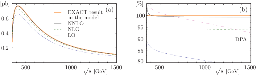
Figure 1: The total cross-section: the exact result in the model and the results of computations in MPT.

$\quad\sqrt{s}$ (TeV)	$\qquad\sigma_{\,\mbox{\tiny EXACT}}\qquad$	$\qquad\sigma_{LO}\qquad$	$\qquad\sigma_{NLO}\qquad$	$\quad\sigma_{NNLO}\qquad$
0.5	0.6724	0.5687	0.6344	0.6698(7)
	100%	84.6%	94.3%	99.6(1)%
1	0.2255	0.1821	0.2124	0.2240(2)
	100%	80.8%	94.2%	99.3(1)%

The outcomes of the computations are presented in the Figure and in the Table. In the Figure in the panel (a) the thick curve shows the behavior of the total cross-section in the model. The dotted, dashed, and continuous thin curves show the results of the MPT computations in the LO, NLO, and NNLO approximations, respectively. It is worth noting that the NNLO result almost coincides with the exact result in the model. The distinction is visible in the panel (b) where the percentages with respect to the exact result are presented. In the Table the outcomes are represented in the numerical form at the characteristic energies planned at the ILC [3]. In the last column the numbers in parenthesis represent the uncertainties in the last digit. In other columns the uncertainties are omitted as they appear beyond the precision of the presentation of data.

In conclusion, first of all the above results show in practice the existence of the MPT expansion in the case of pair production and decay of fundamental unstable particles. Secondly, the NLO and NNLO approximations in the MPT have very stable behavior at the energies near the maximum of the cross-section and at higher energies (and this result to a large extent is model-independent [11]). Thirdly, at the ILC energies the NNLO approximation in the MPT in the case of the top-quark pair production provides approximately a half-percent accuracy of the description of the cross-section. In fact this is what is needed at the ILC. However, the higher precision of the MPT description, when needed, may be achieved by the proceeding to the NNNLO, or by the using of the NNLO for the calculation of the loop contributions only—on the analogy of actual practice of application of DPA [1]. The higher precision of the actual computations in the NNLO of MPT may be achieved at the proceeding to the representation of real numbers with higher precision (higher than with the double precision).

The author is grateful to A.L.Kataev for encouragement and suggestion to make a report at the ACAT Workshop.

References

- [1] W. Beenakker et al., Physics at LEP2 (eds. G.Altarelli et. al., Geneva, 1996) CERN 96-01, Vol. 1, p. 79, hep-ph/9602351; M. Grunewald et al. Four-fermion production in electron-positron collisions. Four-Fermion Working Group (The LEP2-MC workshop 1999/2000), hep-ph/0005309.
-
[2]
A. Denner, S. Dittmaier, M. Roth, L.H. Wieders, Phys. Lett. B612 (2005) 223;
A. Denner, S. Dittmaier, M. Roth, L.H. Wieders, Nucl. Phys. B724 (2005) 247. - [3] J. Brau et al., arXive:0712.1950.
- [4] J. Papavassiliou, A. Pilaftsis, Phys. Rev. Lett. 75 (1995) 3060; D. Binosi, J. Papavassiliou, Phys. Rev. D66 (2002) 111901.
- [5] S. Dittmaier, Proc. of International Europhysics Conference on High-Energy Physics (Jerusalem 1997) p. 709 [hep-ph/9710542].
- [6] F.V. Tkachov, Proc. of the 32nd PNPI Winter School on Nuclear and Particle Physics, St.Petersburg, St.Petersburg, PNPI, 1999, p. 166 [hep-ph/9802307].
- [7] M.L. Nekrasov, Eur. Phys. J. C19 (2001) 441.
- [8] M.L. Nekrasov, Int. Mod. Phys. A24 (2009) 6071.
- [9] M.L. Nekrasov, Plys. Lett. B531 (2002) 225.
- [10] B.A. Kniehl, A. Sirlin, Phys. Lett. B530 (2002) 129.
- [11] M.L. Nekrasov, arXiv:0912.1025.
-
[12]
V.S. Fadin, V.A. Khoze, Proc. of 24th Winter School of LNPI,
Leningrad, LNPI, 1989, vol. I, p. 3;
D. Bardin, W. Beenakker, and A. Denner, Phys. Lett. B317 (1993) 213;
V.S. Fadin, V.A. Khoze, A.D. Martin and A.Chapovsky, Phys. Rev. D52 (1995) 1377.