Semiclassical study of edge states and transverse electron focusing for strong spin-orbit coupling

Abstract

We studied the edge states and transverse electron focusing in the presence of spin-orbit interaction in a two dimensional electron gas. Assuming strong spin-orbit coupling we derived semiclassical quantization conditions to describe the dispersion of the edge states. Using the disprsion relation we then make predictions about certain properties of the focusing spectrum. Comparison of our analytical results with quantum mechanical transport calculations reveals that certain features of the focusing spectrum can be quite well understood in terms of the interference of the edge states while the explanation of other features seems to require a different approach.

I Introduction

Semiclassical approximations are often very practical for understanding certain physical phenomena. Beyond their practicality, they also provide a rather general framework to treat quantum systems of interest. A good example to illustrate the merits of semiclassical approach is the transverse electron focusing (TEF). The geometry of electron focusing is shown in Fig.1. The current is injected into the sample at a quantum point contact called injector (I) in perpendicular magnetic field $\mathcal{B}$. If the magnetic field is an integer multiple of a focusing field $B_{focus}$, electrons injected within a small angle around the perpendicular direction to the edge of the sample can be focused onto a collector quantum point contact (denoted by $C$ in Fig. 1) which acts as a voltage probe. Therefore, if the collector voltage is plotted as a function of magnetic field one can observe equidistant peaks at magnetic fields $B=p*B_{focus}$ ($p=1,2,3,\dots$) corresponding to cases where the cyclotron diameter $2R_{c}(\mathcal{B})$ is an integer multiple of the distance $L$ between the injector and the collector.

TEF is a versatile experimental technique (for a review of the various problems where it has been used see Ref. tsoi, ). In the case of quantum wells containing two dimensional electron gas (2DEG), the accessibility of the quantum ballistic transport regime opened up the way to the experimental demonstration of coherent electron focusingHouten_Carlo ; lu as well. Recently, several experiments investigated the effect of spin-split bands in semiconductors on magnetic focusingpotok ; ref:rokhinson ; dedigama . Of special interest are for us the experiments of Refs. ref:rokhinson, ; dedigama, in which evidence of spin-orbit interaction (SOI) dependent focusing have been found. These experiments sparked considerable theoretical interestusaj ; reynoso-2 ; zulicke ; schliemann as well. Refs. usaj, ; reynoso-2, ; zulicke, ; schliemann, have in common that they consider the properties of bulk Landau levels in the presence of SOI to explain the experimental results on focusing. While using the bulk Landau levels as a starting point is certainly justified when discussing magneto-oscillationskeppeler-1 ; lagenbuch , for the geometry shown in Fig. 1 one expects that the edge states should play a central role in the transport phenomena. Indeed, this was the approach adopted in Ref. Houten_Carlo, to discuss coherent electron focusing. The rich physics brought about by the interplay of SOI and the confinement due to external magnetic field and electrostatic potential has also attracted significant theoretical attentionwang ; pala ; reynoso-1 ; debald ; yun-juan ; grigoryan but implications on electron focusing have not been considered.

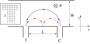
Figure 1: (color online) Schematic geometry of the transverse electron focusing setup. The 2DEG is contacted by an injector (I) and a collector (C) probe and perpendicular magnetic field is applied. Classical quasiparticle trajectories leaving from the injector at normal direction, depending on the strenght of the magnetic field, can be focused onto the collector. The inset shows the details of the tight-binding model used to describe the the probes (c.f. the inset of Fig. 1 in Ref. usaj, ).

Here we aim to investigate whether the electron focusing spectrum in 2DEG with strong SOI can be explained in terms of edge states formed as a combined effect of SOI, magnetic field and (an assumed) hard wall confinement potential. To this end we first derive semiclassical quantization conditions which describe the dispersion relation of the edge states in the limit of strong SOI and weak magnetic fields. These results shed new light on and help to better understand the exact quantum solution of this problem, published very recently in Ref. grigoryan, . We then study how the properties of the edge states are manifested in the transport phenomena of the focusing setup shown in Fig. 1. We expect that our results should be relevant in the case of e.g. InSb quantum wells, where theoretical predictionsgilbertson-2 and recent experimentshong ; dedigama ; khodaparast ; gilbertson-1 indicate that it is possible to fabricate samples with strong (compared to GaAs/AlGaAs heterostructures) spin orbit interaction and ballistic quasiparticle propagation over distances of the order of $1\mu{\rm m}$ at low temperatures.

The rest of the paper is organized in the following way: in the next section we briefly introduce the semiclassical framework that we will be using. In Section III we derive a pair of semiclassical quantization conditions for the edge states and compare the obtained band structure to the results of exact numerical calculations. We also discuss how our semiclassical results are related to other approximation methods found in the literature. The semiclassical quantization conditions then allows us in Section IV to make prediction about the focusing spectrum. We end our paper by a comparison of these predictions to numerical transport calculations and a short summary in Section V.

II Semiclassical theory with spin degrees of freedom

Generally, the non-relativistic single-particle Hamiltonian of spin $1/2$ particles can be written asamand

$$\hat{H}=\hat{H}_{0}+\hat{H}_{1},\quad\hat{H}_{0}=\frac{\hat{\mathbf{p}}^{2}}{2m^{*}}+V(\mathbf{r})$$ (1)

where $\mathbf{r}$ and $\hat{\mathbf{p}}$ denotes the position and momentum operators, respectively, $m^{*}$ is the effective mass of the particles and we assume that the spin dependent part have the following form:

$$\hat{H}_{1}=\hbar\,\kappa\,\widehat{C}(\mathbf{r},\hat{\mathbf{p}})\cdot\boldsymbol{\sigma}.$$ (2)

Here $\boldsymbol{\sigma}=(\sigma_{x},\sigma_{y},\sigma_{z})$ is a vector of Pauli matrices and the $\hbar$ comes from the spin operator $\hat{\mathbf{s}}=\frac{1}{2}\hbar\boldsymbol{\sigma}$. The constant $\kappa$ gives the spin orbit coupling.

The application of semiclassical methods developed for systems that can be described by scalar Hamiltoniansbrackkonyv is not straightforward if one has to consider the spin degree of freedom as well. Namely, as a first step one would have to define a classical Hamiltonian which is not a trivial task since there is no classical analogue of the spin. Various semiclassical schemes have been proposed, see Refs. littlejohn, ; bolte, ; pletyukov, ; keppeler-2, , and we refer to these original papers for most of the details. A short overview of the different approaches can also be found in Refs. amand, ; zulicke, .

Here we will follow the approach first used by Yabana and Horiuchiyabana and later generalized and further developed in Refs. littlejohn, ; bolte, ; keppeler-2, ; gyorffy, ; samokhin, . It is often called the “strong coupling limit” because it corresponds to a double limit $\hbar\rightarrow 0$ and $\kappa\rightarrow\infty$ while $\bar{\kappa}=\hbar\kappa$ is kept constantamand . For spin $1/2$ particles this approximation scheme leads to two classical Hamiltonians

$$\mathcal{H}^{\pm}=\mathcal{H}_{0}\pm\bar{\kappa}|\mathcal{C}(\mathbf{r},\mathbf{p})|$$ (3)

where the vector $\mathcal{C}(\mathbf{r},\mathbf{p})$ is the phase-space symbol of the operator $\widehat{C}(\mathbf{r},\hat{\mathbf{p}})$littlejohn ; keppeler-2 and represents an effective magnetic field which depends on the classical variables $\mathbf{r},\mathbf{p}$. This approximation introduces semiclassical phase corrections to the orbital motionyabana ; littlejohn . It is restricted however to the case of $|\mathcal{C}(\mathbf{r},\mathbf{p})|>0$ because at phase-space points where $|\mathcal{C}(\mathbf{r},\mathbf{p})|$ vanishes and therefore $\mathcal{H}^{\pm}$ becomes degenerate, mode conversion between trajectories described by $\mathcal{H}^{\pm}$ occurs, posing a serious difficulty to the theory.

For a two dimensional electron gas (2DEG) in perpendicular magnetic field and assuming that $\hat{H}_{1}$ describes Rashba-type spin-orbit coupling, which will be our main interest in the rest of the paper, the “strong coupling” approach results in the following semiclassical Landau-level spectrumamand ; reynoso-1 :

$$E_{n}^{s}=\hbar\omega_{c}\left[n\pm\sqrt{2\,n}\,k_{so}l_{B}\right],\,\,\,n=1,2,\dots$$ (4)

where $\omega_{c}=\frac{e\mathcal{B}}{m^{*}}$ is the classical cyclotron frequency, $l_{B}=\sqrt{\hbar/e\mathcal{B}}$ is the magnetic length, and by using the notation $\alpha_{R}$ for the coupling constant $\bar{\kappa}$ in this particular case, $k_{so}$ is given by $k_{so}=m^{*}\alpha_{R}/\hbar$. Comparing this to the exact resultref:bychkov

$$E_{0} = \hbar\omega_{c}/2;$$

$$E_{n} = \hbar\omega_{c}\left[n\pm\sqrt{2\,n\,(k_{so}l_{B})^{2}+\frac{1}{4}}\,\right]$$ (5)

we see that the semiclassical Landau levels are good approximations of the exact ones if $2n(k_{so}l_{B})^{2}\gg 1/4$. This requires large quantum numbers $n$ (i.e. large Fermi energy) and/or strong spin-orbit coupling $\alpha_{R}$ and not too strong magnetic field (i.e. $l_{B}\sim 1/\sqrt{\mathcal{B}}$ is not too small). We expect therefore that the strong coupling method should be adequate if these conditions are met. An estimate of the appropriate magnetic field range assuming InSb quantum well material parameters will be given after Eq. (21b).

III Semiclassical theory of edge states

We assume that the 2DEG, formed e.g. in the quantum well of an InSb heterostructure, is in a perpendicular homogeneous magnetic field. The motion of electrons is confined by a hard-wall potential, $V(y)=\infty$ for $y<0$ (see Fig.1 for the geometry). The quantum mechanical description of the system can be obtained using the Hamiltonian (1) where $\hat{H}_{0}=\frac{\hat{\boldsymbol{\pi}}^{2}}{2m^{*}}$ corresponds to the kinetic energy of particles and the operator $\hat{\boldsymbol{\pi}}$ is defined as $\hat{\boldsymbol{\pi}}=(\hat{\pi}_{x},\hat{\pi}_{y})=\hat{\mathbf{p}}+e\mathbf{A}$, where $\hat{\mathbf{p}}=-i\hbar\boldsymbol{\nabla}$ is the canonical momentum operator and $\mathbf{A}$ is the vector potential. Furthermore, $H_{1}=\alpha_{R}(\hat{\pi}_{x}\sigma_{y}-\hat{\pi}_{y}\sigma_{x})$ describes the Rashba spin-orbit (RSO) coupling in the system, $\sigma_{x}$, $\sigma_{y}$ are Pauli matrices acting in the spin space. We assume that $\alpha_{R}$ is constant in space and neglect its possible random variaton due to nanosize domainssherman .

To preserve the translational invariance of the system, we choose the Landau gauge $\mathbf{A}=(\mathcal{B}y,0,0)^{T}$. Using the ansatz $\Psi(\mathbf{r})=e^{ikx}\Phi(y)$ we can simplify the problem to an effectively one dimensional (1D) one, which we will solve in semiclassical approximation. The discussion goes along the lines of Refs. yabana, ; keppeler-2, ; gyorffy, [for a recent application see also Refs. carmiere, ; sajat2, ]. We seek the solutions of the 1D Schrödinger equation $\hat{H}\Phi(y)=E\Phi(y)$ in the following form keppeler-2 :

$$\Phi(y)=\sum_{q\geq 0}\left(\frac{\hbar}{i}\right)^{q}\mathbf{a}_{q}(y)e^{\frac{i}{\hbar}S(y)},$$ (6)

where $\mathbf{a}_{q}(y)$ are spinors and $S(y)$ is the classical action. Performing the unitary transformation $\Phi\rightarrow e^{-\frac{i}{\hbar}S(y)}\Phi(y)$, $\hat{H}\rightarrow e^{-\frac{i}{\hbar}S(y)}\hat{H}\,e^{\frac{i}{\hbar}S(y)}$ the Schrödinger equation can be rewritten as

$$\begin{split}\left(\begin{array}[]{cc}\frac{\hat{\Pi}_{x}^{2}+\hat{\Pi}_{y}^{2}}{2m^{*}}-{E}&i\alpha_{R}(\hat{\Pi}_{x}-i\hat{\Pi}_{y})\\ -i\alpha_{R}(\hat{\Pi}_{x}+i\hat{\Pi}_{y})&\frac{\hat{\Pi}_{x}^{2}+\hat{\Pi}_{y}^{2}}{2m^{*}}-{E}\end{array}\right)\left(\mathbf{a}_{0}(y)\right.+\\ \left.\frac{\hbar}{i}\mathbf{a}_{1}(y)+\dots\right)=0.\end{split}$$ (7)

Here $\hat{\Pi}_{x}\equiv\Pi^{0}_{x}=p_{x}+eA_{x}(\mathbf{r})$, $p_{x}$ being $p_{x}=\hbar k$, and $\hat{\Pi}_{y}=\hat{p}_{y}+\Pi^{0}_{y}$, where $\Pi^{0}_{y}=\frac{\partial S(y)}{\partial y}$. The WKB strategybrackkonyv is to satisfy Eq. (7) separately order by order in $\hbar$.

At $\mathcal{O}(\hbar^{0})$ order we obtain

$$\left(\begin{array}[]{cc}\frac{(\Pi_{x}^{0})^{2}+(\Pi_{y}^{0})^{2}}{2m^{*}}-{E}&i\alpha_{R}({\Pi}_{x}^{0}-i{\Pi}_{y}^{0})\\ -i\alpha_{R}({\Pi}_{x}^{0}+i{\Pi}_{y}^{0})&\frac{(\Pi_{x}^{0})^{2}+(\Pi_{y}^{0})^{2}}{2m^{*}}-{E}\end{array}\right)\mathbf{a}_{0}(y)=0.$$ (8)

Nontrivial zeroth order eigenvectors $\mathbf{a}_{0}(y)$ exist if

$$E=\frac{Q^{2}}{2m^{*}}\pm\alpha_{R}\,Q$$ (9)

where $Q=\sqrt{(\Pi_{x}^{0})^{2}+(\Pi_{y}^{0})^{2}}$. This means that $Q$ is a constant of motion for a given energy $E$ and the two branches of Eq. (9) define

$$Q_{-}=\sqrt{p_{so}^{2}+2m^{*}E}-p_{so}$$ (10a)

$$Q_{+}=p_{so}+\sqrt{p_{so}^{2}+2m^{*}E}$$ (10b)

where we used the notation $p_{so}=m^{*}\alpha_{R}$. We find therefore that the classical equations of motion that can be derived from Eqs. (9) and (10b) represent two harmonic oscillators. The corresponding zeroth order eigenvectors of Eq. (8) are

$$\mathbf{V}_{\pm}=\frac{1}{\sqrt{2}}\left(\begin{array}[]{c}e^{-\frac{i}{2}(\theta(y)\mp\pi/2)}\\ e^{\frac{i}{2}(\theta(y)\mp\pi/2)}\end{array}\right)$$ (11)

where $\theta(y)$ is the phase of $\Pi_{x}^{0}(y)-i\Pi_{y}^{0}(y)$. However, the eigenspinor $\mathbf{a}_{0}(y)^{\pm}$ can more generally be sought as $\mathbf{a}_{0}^{\pm}=\mathcal{A}_{\pm}(y)e^{i\gamma_{\pm}(y)}\mathbf{V}_{\pm}$ where $\mathcal{A}_{\pm}(y)$ is a real amplitude and $\gamma_{\pm}(y)$ is a phase. Equations for $\mathcal{A}_{\pm}(y)$ and $\gamma_{\pm}(y)$ can be obtained from the $\mathcal{O}(\hbar^{1})$ order of Eq. (7). Using Eq. (11) we find that the $\mathcal{O}(\hbar^{1})$ order equation can be cast into the following form:

$$\overrightarrow{\nabla}\left(\frac{\mathcal{A}_{\pm}^{2}}{2}\left[\frac{1}{m^{*}}\left(\begin{array}[]{c}\Pi_{x}^{0}\\ \Pi_{y}^{0}\end{array}\right)\pm\alpha_{R}\left(\begin{array}[]{c}\cos\theta(y)\\ \sin\theta(y)\end{array}\right)\right]\right)=0.$$ (12)

This equation does not depend on $\gamma_{\pm}$, which means that with the choice of the eigenvectors shown in Eq. (11), the phase $\gamma_{\pm}(y)$ is already determined up to an unimportant constant factor. Moreover, by rewriting Eq. (12) as

$$\overrightarrow{\nabla}\left(\frac{\mathcal{A}_{\pm}^{2}}{2}\frac{\partial\mathcal{H}^{\pm}}{\partial\mathbf{p}}\right)=0$$ (13)

where $\mathcal{H}^{\pm}=Q^{2}/2m^{2}\pm\alpha_{R}\,Q$, it is easy to see that it expresses probability current conservation and it can be solved for $\mathcal{A}_{\pm}$ using standard methodsbrackkonyv . From these results one finds that $\Phi(y)$ in semiclassical approximation is given by

$$\Phi^{\pm}(y)=\frac{1}{\sqrt{2|\Pi_{y}^{0,\pm}|}}\left(\begin{array}[]{c}e^{-\frac{i}{2}(\theta^{\pm}(y)\mp\pi/2)}\\ e^{\frac{i}{2}(\theta^{\pm}(y)\mp\pi/2))}\end{array}\right)e^{\frac{i}{\hbar}S(y,y_{0}^{\pm})}$$ (14)

where $|\Pi_{y}^{0,\pm}|=\sqrt{Q_{\pm}^{2}-(\Pi_{x}^{0})^{2}}.$ However, as the momentum $\Pi_{y}^{0,\pm}$ is a multi-valued function, we need to introduce the index $j=+1,-1$ do distinguish the different branches. The corresponding classical actions $S_{j}^{\pm}(y,y_{0}^{\pm})$ read

$$S_{j}^{\pm}(y,y_{0}^{\pm})=j\int_{y_{0}^{\pm}}^{y}\sqrt{Q_{\pm}^{2}-[\Pi_{x}^{0}(y^{\prime})]^{2}}\,{\rm d}y^{\prime}$$ (15)

where as usually, we have chosen the classical turning points as the phase reference points for the action. Similarly, the phase $\theta^{\pm}(y)=\theta_{j}^{\pm}(y)$ is multivalued as well.

We now have to take into account the confinement potential $V(y)$. The transverse wavefunctions $\Phi(y)$ shown in Eq. (14) would not satisfy the boundary condition at $y=0$. In order that the transverse wavefunction does satisfy the boundary condition we make a linear combination of the functions $\Phi_{j}^{\pm}(y)$ defined above. We try the following ansatz for the transverse semiclassical wavefunction:

$$\begin{split}\tilde{\Phi}(y)=&\frac{\mathcal{C}_{+}}{\sqrt{|\Pi_{y}^{0,+}(y)|}}\left(\begin{array}[]{c}e^{i\frac{\pi}{4}}\cos\left(\frac{S_{0}^{+}(y,y_{0}^{+})}{\hbar}-\frac{\theta^{+}(y)}{2}+\frac{\pi}{4}\right)\\ e^{-i\frac{\pi}{4}}\cos\left(\frac{S_{0}^{+}(y,y_{0}^{+})}{\hbar}+\frac{\theta^{+}(y)}{2}+\frac{\pi}{4}\right)\end{array}\right)+\\ &\frac{\mathcal{C}_{-}}{\sqrt{|\Pi_{y}^{0,-}(y)|}}\left(\begin{array}[]{c}e^{-i\frac{\pi}{4}}\cos\left(\frac{S_{0}^{-}(y,y_{0}^{-})}{\hbar}-\frac{\theta^{-}(y)}{2}+\frac{\pi}{4}\right)\\ e^{+i\frac{\pi}{4}}\cos\left(\frac{S_{0}^{-}(y,y_{0}^{-})}{\hbar}+\frac{\theta^{-}(y)}{2}+\frac{\pi}{4}\right)\end{array}\right)\end{split}$$ (16)

where $\mathcal{C}_{+}$, $\mathcal{C}_{-}$ are constants and the $\pi/4$ factor in the argument of the cosine functions takes into account the effect of the classical turning points at $y_{0}^{\pm}$ which appear due to the magnetic field. The turning points are given by the physically acceptable zeros of the equation $Q_{\pm}^{2}-[\Pi_{x}^{0}(y^{\prime})]^{2}=0$. Note that $\tilde{\Phi}(y)$ also depends on $k$ through $S_{0}^{\pm}$ and $\theta^{\pm}$ but in order to keep the notations uncluttered we did not write this out explicitly. The dispersion relation for the edge states can be obtained by demanding that the wave function vanishes at the boundary, i.e. $\tilde{\Phi}(y=0)=0$. This is a homogeneous system of equations and nontrivial solutions can only be found if the respective determinant is zero. This results in the following implicit dispersion relation:

$$\begin{array}[]{c}\cos\left(\frac{S_{0}^{+}(0,y_{0}^{+})}{\hbar}-\frac{\theta^{+}(0)}{2}+\frac{\pi}{4}\right)\cos\left(\frac{S_{0}^{-}(0,y_{0}^{-})}{\hbar}+\frac{\theta^{-}(0)}{2}+\frac{\pi}{4}\right)+\\ \cos\left(\frac{S_{0}^{-}(0,y_{0}^{-})}{\hbar}-\frac{\theta^{-}(0)}{2}+\frac{\pi}{4}\right)\cos\left(\frac{S_{0}^{+}(0,y_{0}^{+})}{\hbar}+\frac{\theta^{+}(0)}{2}+\frac{\pi}{4}\right)=0.\end{array}$$ (17)

Hence, if we denote by $\tilde{\Phi}^{+}(y)$ and $\tilde{\Phi}^{-}(y)$ the first and second spinors appearing in Eq. (16), respectively, the transverse wave function can be written, apart from a normalization factor, as $\tilde{\Phi}(y)\sim\tilde{\Phi}^{+}(y)+r_{so}\,\tilde{\Phi}^{-}(y)$ where $r_{so}$ is given by

$$r_{so}=-e^{i\frac{\pi}{2}}\sqrt{\frac{|\Pi_{y}^{0,-}(0)|}{|\Pi_{y}^{0,+}(0)|}}\frac{\cos\left(\frac{S_{0}^{+}(0,y_{0}^{+})}{\hbar}-\frac{\theta^{+}(0)}{2}+\frac{\pi}{4}\right)}{\cos\left(\frac{S_{0}^{-}(0,y_{0}^{-})}{\hbar}-\frac{\theta^{-}(0)}{2}+\frac{\pi}{4}\right)}.$$ (18)

For $k\approx 0$ the reflection amplitude is $r_{so}\approx-e^{i\pi/2}$.

Furthermore, with the help of trigonometric identities and assuming that

$$\begin{array}[]{c}\cos\left(\frac{S_{0}^{+}(0,y_{0}^{+})}{\hbar}-\frac{S_{0}^{-}(0,y_{0}^{-})}{\hbar}\right)\approx\cos\left(\frac{\theta^{+}(0)}{2}-\frac{\theta^{-}(0)}{2}\right)\approx 1\end{array}$$ (19)

we find from Eq. (17) the following quantization condition:

$$\begin{array}[]{c}\cos\left(\frac{\Lambda_{+}+\Lambda_{-}+\varphi_{+}+\varphi_{-}}{2}\right)\cos\left(\frac{\Lambda_{+}+\Lambda_{-}-\varphi_{+}-\varphi_{-}}{2}\right)=0\end{array}$$ (20)

where for brevity we introduced the notations $\Lambda_{\pm}=\frac{S_{0}^{\pm}(0,y_{0}^{\pm})}{\hbar}+\pi/4$ and $\varphi_{\pm}=\frac{\theta^{\pm}(0)}{2}$. Here we pause for a moment to interpret Eq. (19). From the discussion below Eq. (10b) and from Eq. (15) it is clear that if we consider the two branches of Eq. (9) as classical Hamiltonians for two different quasiparticles then $S_{0}^{\pm}(0,y_{0}^{\pm})$ gives (half of the) enclosed flux by the quasiparticle trajectories with the wall between two subsequent collisions and $\theta^{\pm}(0)$ is the deflection angle of the momentum between the collisions. Therefore Eq. (19) means that we neglect the second and higher powers of the difference between the enclosed flux and momentum deflection.

It is clear that Eq. (20) defines a pair of quantization conditions: $\Lambda_{+}+\Lambda_{-}+\varphi_{+}+\varphi_{-}=(2m+1)\pi$ and $\Lambda_{+}+\Lambda_{-}-\varphi_{+}-\varphi_{-}=(2l+1)\pi$ with $l,m=0,1,2,\dots$. By introducing the angle $\beta_{\pm}=\arcsin\left(\frac{X}{R_{\pm}}\right)$, where $X=kl_{B}^{2}$ is the guiding center coordinate and $R_{\pm}=Q_{\pm}/(e\mathcal{B})$ is the radius of the cyclotron motion for the two quasiparticle branch, we finally arrive at the following two quantization conditions:

$$\begin{split}\frac{R_{+}^{2}}{l_{B}^{2}}\left(\frac{1}{2}\sin 2\beta_{+}+\beta_{+}+\frac{\pi}{2}\right)+\frac{R_{-}^{2}}{l_{B}^{2}}\left(\frac{1}{2}\sin 2\beta_{-}+\beta_{-}+\frac{\pi}{2}\right)+\\ \left(\beta_{+}+\beta_{-}\right)=4\pi m,\quad m=0,1,\dots m_{max}\end{split}$$ (21a)

and

$$\begin{split}\frac{R_{+}^{2}}{l_{B}^{2}}\left(\frac{1}{2}\sin 2\beta_{+}+\beta_{+}+\frac{\pi}{2}\right)+\frac{R_{-}^{2}}{l_{B}^{2}}\left(\frac{1}{2}\sin 2\beta_{-}+\beta_{-}+\frac{\pi}{2}\right)+\\ (\pi-\beta_{+})+(\pi-\beta_{-})=4\pi l,\quad l=0,1,\dots l_{max}\end{split}$$ (21b)

These equations are the first important results of our paper. They do not lend themselves to a simple semiclassical interpretation but a possible classical picture could be the following: the classical skipping orbits whose quantization would be described by these equations consist of two segments, each of them having slightly different radii given by $R_{\pm}$ but the same guiding center coordinate. Besides the orbital motion, the quantization conditions also depend on the change of the phase of the spinor part of the wavefunction which is described by the $(\beta_{+}+\beta_{-})$, $(\pi-\beta_{+})+(\pi-\beta_{-})$ terms in Eqs. (21b).

We note that analogous calculations to the ones outlined above can be carried out if the dominant term in the SOI is the $k$-linear Dresselhaus term. Therefore this approach can be relevant e.g. in the case of heterostructure studied in Ref. akabori, .

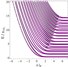
Figure 2: (color online) Comparison of the dispersion of the bands as a function of the wavenumber $k$ obtained from tight-binding numerical calculations (dots), and using the theoretical prediction given by Eqs. (21b) (solid lines) for magnetic field $\mathcal{B}=0.15{\rm T}$ and $k_{so}l_{B}=0.256$ (other parameters are given in the text). The dashed line at the leftmost band shows the result of Eq. (22) for $m=0$.

To see the accuracy of the semiclassical quantization we have performed numerical calculations for the dispersion of the edge states using the tight-binding version of the Hamiltonian (1) [see e.g. Ref. reynoso-2, for the explicit form of the tight-binding Hamiltonian]. The results for $k_{so}l_{B}=0.256$ at a relatively weak magnetic field of $\mathcal{B}=0.15{\rm T}$ and using typical parameters of 2DEG in InSb quantum well at higher electron densitiesgilbertson-2 ($m^{*}=0.021\,m_{e}$, where $m_{e}$ is the bare electron mass and $\alpha_{R}=1.4*10^{-11}\,{\rm eVm}$) are shown in Fig. 2. As one can see Eqs. (21b) describe quite well the dispersion of the subbands, even at low energies, except for the $k$ values where the guiding center $X\approx R_{\pm}$, i.e. in the transition region to the bulk Landau levels. We have found that although Eqs. (21b) have solutions even for $m=0$ and $l=0$, the leftmost band in Fig. 2, which is related to the zeroth Landau level, is poorly approximated by any of the $m=0$ or $l=0$ curves that can be obtained from Eq. (21a) or Eq. (21b), respectively. Nevertheless, the approximation works quite well for rest of the subbands, i.e. for $m,l\geq 1$. For a stronger magnetic field of $\mathcal{B}=0.6{\rm T}$ ($k_{so}l_{B}=0.128$) shown in Fig. 3, the approximation for the $m=1$ and $l=1$ bands deteriorated as well, while higher subbands are still well described by Eq. (21b).

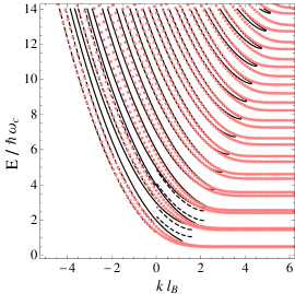
Figure 3: (color online) Comparison of the dispersion of the bands as a function of the wavenumber $k$ obtained from tight-binding numerical calculations (dots), and using the theoretical prediction given by Eqs. (21b) (solid lines) for magnetic field $\mathcal{B}=0.6{\rm T}$ and $k_{so}l_{B}=0.128$ (other parameters are given in the text). Dashed lines at the leftmost bands show the result of Eqs. (22) for $m=0,1$.

It is interesting to note that we find that the bands for $0\ll|X|\lesssim R_{\pm}$ are quite well approximated by the following simple formulae:

$$\frac{R_{\pm}^{2}}{l_{B}^{2}}\left(\frac{1}{2}\sin 2\beta_{\pm}+\beta_{\pm}+\frac{\pi}{2}\right)-\pi\Theta(X)=2\pi(m+3/4)$$ (22)

where $\Theta(x)=1$ for $x>0$ and zero otherwise. Note that in contrast to Eqs. (21b) these equations give a semiclassical quantization of the orbital motion of two independent systems whose classical motion is described by the Hamiltonians $\mathcal{H}^{\pm}$ given by the left-hand side of Eq. (9). The spinor nature of the quasiparticles enters the quantization only through a $-\pi$ phase shift for large positive $X$ values. The origin of this phase shift can be understood by looking at Fig. 4. For $-R_{\pm}\lesssim X\ll 0$ the phase contribution coming from the $\pm\exp(i\theta(y)/2)$ factors of the wavefunction (see Eq. (11) is zero over one full period of the classical motion [ Fig. 4(a)]. This happens because the phase change accumulated during the orbital motion $\theta_{out}-\theta_{i}=-2\gamma$ is canceled by the phase change $2\gamma$ upon reflection when the sign of the $\Pi_{y}^{0}$ is negated. However, as it is explained in Fig. 4(b), for orbits with $0\ll X\lesssim R_{\pm}$ the total phase change is $-2\pi/2=-\pi$. We find that the leftmost band in Fig. 2 which is related to the zeroth bulk Landau level (see Eq. 5) can be quite well approximated by the $-$ branch of Eq. 22 for $m=0$. For stronger magnetic fields, such as shown in Fig. 3, the left-most bands are better approximated by the quantization (22) than by Eqs. (21b). We note that for $X<0$ the quantization in Eq. (22) basically corresponds to the “longitudinal SO approximation” studied in Ref. pala, .

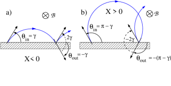
Figure 4: (color online) Explanation of the phase shift $-\pi$ for $X>0$ in Eq. (22). Solid (blue) lines show the bent quasiparticle trajectories. The direction of the momentum at the start of a full period and at the subsequent collision with the wall is indicated by arrows. Also shown are the angles that the momentum encloses with the wall. The phase shift contribution coming from the spinor part of the semiclassical wavefunction is $\frac{1}{2}(\theta_{out}-\theta_{in}+2\gamma)$ in (a) and $\frac{1}{2}(\theta_{out}-\theta_{in}-2\gamma)$ in (b).

Another interesting and important comparison of the quantization shown in Eqs. (21b) can be made to the closely related results of Ref. reynoso-2, , where the authors used a different semiclassical approachpletyukov to describe the edge states in the presence of RSO. Firstly, we find the same result for the $k=0$ energy levels as in Ref. reynoso-2, :

$$E_{m}(k=0)=\hbar\omega_{c}(n-(k_{so}l_{B})^{2})$$ (23)

and a comparison with the numerical calculations show that it is a good approximation of the exact results. However, we obtained a pair of quantization conditions, not just one [see Eq. (27) in Ref. reynoso-2, ]. Furthermore, for the parameter range we consider our results give a good approximation of the numerically calculated bands not only close to $k=0$ but for the whole dispersion relation. Finally, an important difference in the semiclassical interpretation of the skipping orbits is the following: in the classical picture put forward in Ref. reynoso-2, the skipping orbits consist of two different type of arcs, having radii $R_{\pm}$ and guiding center coordinates $X_{\pm}$. Moreover, the guiding center changes upon each reflection at the wall (see Fig.6 in Ref. reynoso-2, ). In contrast, our approach tells that the guiding center remains the same throughout the motion. We think that this is physically plausible because the guiding center is a constant of motion. It is instead the reflection angle that slightly changes at each collision with the wall as a consequence of having two Fermi surfaces with different radii.

IV Magnetic focusing

Having obtained the quantization condition for edge states in Eqs. (21b), the calculation of the focusing magnetic fields $B_{focus}$ goes along the lines of the discussion of Ref. Houten_Carlo, . We expect that the ballistic transport in a mesoscopic wire in the magnetic field regime where the cyclotron diameter is smaller then the wire width can be understood in terms of the edge states described in Section III because they are the propagating modes of this problem. If the injector is narrow, i.e. it is only a few Fermi wavelength wide, one can assume that it excites these modes coherently. Therefore, as long as the distance between the injector and the collector is smaller than the mean free path (and phase coherence lenght), the interference of the edge states can be important. Since the total wave function of the system can be written as a sum of all populated edge states $|k_{m}\rangle$, $|k_{l}\rangle$ at a given Fermi energy, i.e. $\Psi(\mathbf{r})\sim\sum_{l}\mathcal{C}_{l}\tilde{\Phi}(y,k_{l})e^{ik_{l}x}+\sum_{m}\mathcal{C}_{m}\tilde{\Phi}(y,k_{m})e^{ik_{m}x}$ (here $\mathcal{C}_{l}$, $\mathcal{C}_{m}$ are normalization constants), interference along the confinement potential is determined by the phase factors $\exp(ik_{m}x)$, $\exp(ik_{l}x)$. Here the wave numbers $k_{m}$, $k_{l}$ are determined by requiring that they satisfy Eqs. (21a) and (21b) respectively, for a given Fermi energy $E_{F}$ and quantum numbers $m$ and $l$. As in Ref. Houten_Carlo, , we assume that the current at the collector is determined by the unperturbed probability density and therefore the focusing peaks are the results of the constructive interference of edges states with $k_{l,m}\approx 0$ at a distance $x=L$ from the injector. This corresponds to the assumption that only electrons injected close to perpendicular direction can be focused onto the collector. It is convenient to introduce the following notation: $\tilde{R}=R_{+}-R_{-}$, $\tilde{E}_{F}=E_{F}/\hbar\omega_{c}$ and we denote by $k_{F}^{\pm}=Q_{\pm}(E_{F})/\hbar$ the radii of the two Fermi surfaces (circles) in the wavenumber space. Then for $k\ll k_{F}^{\pm}$ we have $1\gg\beta_{\pm}\approx k/k_{F}^{\pm}$ and expanding Eq. (21a) in this small parameter we find that in lowest order

$$k_{m}=\frac{1}{4\tilde{R}\left(1+\frac{1}{\tilde{E}_{F}}\right)}\left(4\pi m-\frac{\pi}{2}[k_{F}^{+}R_{+}+k_{F}^{-}R_{-}]\right).$$ (24a)

Similarly, expanding Eq. (21b) we obtain

$$k_{l}=\frac{1}{4\tilde{R}\left(1-\frac{1}{\tilde{E}_{F}}\right)}\left(2\pi(2l+1)-\frac{\pi}{2}[k_{F}^{+}R_{+}+k_{F}^{-}R_{-}]\right).$$ (24b)

In the semiclassical regime, where $E_{F}\gg\hbar\omega_{c}$ and hence $\tilde{E}_{F}\gg 1$ we can take $\left(1+\frac{1}{\tilde{E}_{F}}\right)\approx\left(1-\frac{1}{\tilde{E}_{F}}\right)\approx 1$. Therefore the phase difference $k_{l}L-k_{m}L$ at distance $L$ from the injector between two edge states whose wavenumbers $k_{m}$ and $k_{l}$ are given by Eq. (24a) and Eq. (24b), respectively, reads

$$k_{l}L-k_{m}L=2\pi(l-m)\frac{L}{2\tilde{R}}+\pi\frac{L}{2\tilde{R}}$$ (25)

and we remind that $\tilde{R}(\mathcal{B})=\sqrt{p_{so}^{2}+2m^{*}E_{F}}/{e\mathcal{B}}$. We see that if for a given magnetic field e.g. $L=2\tilde{R}(\mathcal{B})$ then the phase difference $k_{l}L-k_{m}L$ will be an odd multiple of $\pi$. This means that the spinor part of the wave function of these two edge states, $\tilde{\Phi}(y,k_{l})$ and $\tilde{\Phi}(y,k_{m})$ [see Eq. (16)] will appear with opposite signs in the total wave function, which may lead to a near cancellation of $|k_{m}\rangle$ and $|k_{l}\rangle$.

In general, whenever $L$ is an odd multiple of $2\tilde{R}$, the phase difference will be an odd multiple of $\pi$ meaning that there may be a near cancellation between $|k_{l}\rangle$ and $|k_{m}\rangle$. On the other hand, the phase difference between edge states $|k_{m}\rangle$ and $|k_{m^{{}^{\prime}}}\rangle$, both belonging to the same semiclassical quantization branch given in Eq. (21a) is

$$k_{m}L-k_{m^{{}^{\prime}}}L=2\pi\frac{m-m^{{}^{\prime}}}{\left(1+\frac{1}{4\tilde{E}}\right)}\frac{L}{2\tilde{R}}$$ (26)

and a similar expression can be derived for the phase difference $k_{l}L-k_{l^{{}^{\prime}}}L$ between edge states $|k_{l}\rangle$ and $|k_{l^{{}^{\prime}}}\rangle$ of the other quantization branch [Eq. (21b)]. As long as $\tilde{E}\gg 1$, edge states given by the same quantization branch can interfere constructively at distances $L=q\,2\tilde{R}(\mathcal{B})$, $q=1,2,3,...$ i.e. regardless of whether $L$ is an even or odd multiple of the cyclotron diameter $2\tilde{R}(\mathcal{B})$. By constructive interference we mean that wave function of $|k_{m}\rangle$ and $|k_{m}^{\prime}\rangle$ have the same global sign. (Note however that the $\tilde{E}\gg 1$, i.e. $E_{F}\gg\hbar\omega_{c}$ condition gives an upper limit for the $q$ values for which this reasoning is applicable).

In contrast, if $L$ is an even multiple of $2\tilde{R}$ (e.g. $L=4\tilde{R}$) we find from Eq. (25) that the phase difference $k_{l}L-k_{m}L$ will be an integer multiple of $2\pi$. This means that in this case not only edge states belonging to the same quantization branch but also those belonging to different quantization branches can interfere constructively. Following the reasoning of Ref. Houten_Carlo, therefore we expect that there will be peaks in the focusing spectra for magnetic fields $\mathcal{B}$ where $L$ is even multiple of $2\tilde{R}(\mathcal{B})$ while we might not see peaks at magnetic fields corresponding to $L$ being odd multiple of $2\tilde{R}(\mathcal{B})$. This simple analysis then suggests that the focusing fields are given by integer multiples of $B_{focus}=4\sqrt{2m^{*}E_{F}+p_{so}^{2}}/eL$.

It is interesting to compare these predictions on the focusing spectra to exact numerical transport calculations. Using the tight binding versionreynoso-2 of the Hamiltonian (1), the transmission probability $T_{ic}(\mathcal{B})$ between the injector and collector was calculated by employing the Green’s function technique of Ref. sanvito, . The scattering region was of finite width $W$tightbind-params and was assumed to be perfectly ballistic and infinitely long (see Fig. 1). This means that the left and right ends of it act as drains which absorb any particles exiting to the left of right. The spin orbit coupling had a finite value in the scattering region but was set to zero in the injector and collector. To simulate the effect of finite temperatures we used a simple energy averaging procedure in the calculation of the transmission curves: $T_{ci}(\mathcal{B})=\int T_{ci}(\mathcal{B},E)\left(-\frac{\partial f_{0}(E)}{\partial E}\right)dE$ where $f_{0}(E)$ was the Fermi function. The actual results shown in Fig. 5 were calculated at $T=1K$ temperature. As it can be expected, higher temperatures tend to smear the curves while at lower ones an additional fine structure appears. Our calculations are very similar to those in Ref. usaj, except that we used slightly different contacts (see the inset of Fig. 1). The contacts were always of a finite width (typically five-nine sites wide) and could in principle accommodate more than one (spin-degenerate) open channels.

Figure 5: (color online) a) The transmission from the injector to the collector as a function of the magnetic field. The right inset shows the close-up of the first focusing peak. The left inset shows that if one neglects the Zeeman interaction then the third peak is not split. b) the partial transmissions $T_{c+,i+}$ (solid line) and $T_{c-,i-}$ (dashed line). c) the partial transmissions $T_{c-,i+}$ (solid line) and $T_{c+,i-}$ (dashed line) - in this scale $T_{c-,i+}$ cannot be distinguished from $T_{c+,i-}$. Note the different vertical scale with respect to Fig. 5(b).

Figure. 5(a) shows the transmission $T_{ci}$ a function of the magnetic field $\mathcal{B}$. We used parameter values that approximately correspond to the measurements of Ref. gilbertson-2, on InSb quantum wells: electron density $n_{e}=3.25*10^{15}/m^{2}$, effective mass $m^{*}=0.02\,m_{e}$ and Rashba coefficient $\alpha_{R}=1.4*10^{-11}{\rm eVm}$. It has been shownnedniyom that the effective giromagnetic factor ${\rm g}_{eff}$ of InSb is quite large and therefore the Zeeman spin splitting can be noticeable already at relatively weak magnetic fields. Therefore in our numerical calculation we took into account the Zeeman term as well and assumed ${\rm g}_{eff}=-22$. The distance $L$ was $945{\rm nm}$ and both contacts were tuned to accommodate one (spin-degenerate) open channel. We find that for these parameters the first focusing peak is split [see the right inset of Fig. 5(a)]. That for strong enough $\alpha_{R}$ the first peak is split was first noticed in Ref. usaj, . The peak splitting in good approximation corresponds to $\Delta\mathcal{B}=\frac{4\hbar k_{so}}{eL}\approx 10\,{\rm mT}$. Comparing now the numerical result on the first focusing peak to our analytical prediction, we see that the dip between the peaks is at the magnetic field value where the analytics predicts that destructive interference may take place for $L=2\tilde{R}$ (corresponding to $\mathcal{B}\approx 0.2{\rm T}$) but that the presence of the twin peaks at $\mathcal{B}_{-}=-0.196\,{\rm T}$ and $\mathcal{B}_{+}=-0.206\,{\rm T}$ is not explained by our approach. It appears that the most straightforward way to understand them is to assume spin-split cyclotron orbits, as in Refs. usaj, ; reynoso-1, ; zulicke, . Looking at the second focusing peak, one observes that it is located at $L=4\tilde{R}$ (which happens for $\mathcal{B}=0.4\,{\rm T}$) quite accurately, in accordance with our edge-state based theory. The fact that its amplitude is significantly larger than the amplitude of the first peaks seems to corroborate the theoretical prediction that in this case edge states belonging to different quantization branches [Eq. (21a) and Eq. (21b)] can constructively interfere with each other. Whether this enhancement of the amplitude could be observed in an actual experimental situation, however, depends on how specular the reflection at the confinement potential is. (Note that in the classical picture the second focusing peak correspond to trajectories which bounce off the boundary between the injector and collector once, see the dashed line in Fig. 1.) A small amount of diffuse scattering at the boundary may render the observation of this enhancement difficult. Finally, we find that close to $L=6\tilde{R}$ ($\mathcal{B}=0.597{\rm T}$), where our calculations predict that the wave functions of the edge states may cancel, the amplitude of the transmission is indeed small, but the focusing peak at a slightly higher magnetic field is again not captured by our calculations. It seems that peaks which appear when $L$ is odd multiple of $2\tilde{R}$ can not be described with the presented theoretical approach. The splitting of the third peak close to $\mathcal{B}=-0.62{\rm T}$, reminiscent of the splitting of the first one, is due to the Zeeman interaction and not to the SOI. As we mentioned, because of the large ${\rm g}_{eff}$ the Zeeman energy can be important at smaller magnetic fields than in e.g. GaAs. This is illustrated in the left inset of Fig. 5(a) where we show the calculation for the third peak but without taking into account the Zeeman term in the Hamiltonian. One can see that for the assumed strength of $\alpha_{R}=1.4*10^{-11}{\rm eVm}$ the third peak is not split in this case.

In Fig. 5(b) and (c) we show the partial transmissions assuming spin polarized injection/detection. Thus, e.g. $T_{c+,i-}$ refers to the transmission probability of electrons being injected in spin $-1$ eigenstate and collected in $+1$. In contrast to Ref. usaj, we chose as spin quantization axis the $\hat{y}$ direction (for the definition of the coordinates, see Fig. 1). The motivation to choose this axis comes from Ref. grigoryan, where it was shown that the average spin of the edge states (at least the low energy ones) pointed mainly in the direction perpendicular to the confinement potential, i.e. along the ${y}$ axis in our case. Comparing Fig. 5(b) and (c) one can observe that except for the first focusing peak, the spin-flip transmissions $T_{c+,i-}$, $T_{c-,i+}$ are always significantly smaller than $T_{c+,i+}$, $T_{c-,i-}$. We also performed calculations (not shown here) where the injected electrons were polarized in the $\hat{x}$ direction, as in Ref. usaj, , and we found that $T_{c+,i-}$, $T_{c-,i+}$ were, apart from the vicinity of the first peak, usually smaller in the case of $\hat{y}$ polarized injection than for $\hat{x}$ polarized one. Further investigation of the average polarization of the spin of the edge states in the semiclassical limit and its effect on the partial transmissions in a focusing setup is left to a future work.

V Summary

In summary, we studied the role of edge states in transverse electron focusing setup for strong spin-orbit coupling. As a first step, employing a semiclassical approach we derived a good approximation for the dispersion relation of the edge states and briefly compared our results to other approximation methods that can be found in the literature. We then studied the interference of the edge states as this is expected to have ramifications on the focusing spectrum. Comparison of our theoretical results with numerical transport calculations suggests that certain properties of the focusing spectrum can be quite well understood in terms of the interference of the edge states. Nevertheless, the presented semiclassical approach can not capture all the important characteristics of the transport calculations. Finally, we studied numerically the electron focusing when spin polarized injection was used.

Acknowledgements: A. K. was supported by EPSRC.

References

- (1) V. S. Tsoi, J. Bass, and P. Wyder, Rev. Mod. Phys. 71, 1641 (1999).
- (2) H. van Houten, C. W. J. Beenakker, J. G. Williamson, M. E. I. Broekaart, P. H. M. van Loosdrecht, B. J. van Wees, J. E. Mooij, C. T. Foxon, and J. J. Harris, Phys. Rev. B 39, 8556 (1989).
- (3) J. P. Lu and M. Shayegan, Phys. Rev. B 53, 4217(R) (1996).
- (4) R. M. Potok, J. A. Folk, C. M. Marcus and V. Umansky, Phys. Rev. Lett. 89 266602 (2002).
- (5) L. P. Rokhinson, V. Larkina, Y. B. Lyanda-Geller, L. N. Pfeiffer and K. W. West, Phys. Rev. Lett. 93, 146601 (2004).
- (6) A R. Dedigama, D. Deen, S Q. Murphy, N. Goel, J C. Keay, M. B. Santos, K. Suzuki, S. Miyashita, Y. Hirayama, Physica E 34, 647-650 (2006).
- (7) Gonzalo Usaj and C. A. Balseiro, Phys. Rev. B 70, 041301(R) (2004).
- (8) A. A. Reynoso, Gonzalo Usaj, and C. A. Balseiro, Phys. Rev. B 78, 115312 (2008).
- (9) Ch. Amann and M. Brack, J. Phys. A: Math. Gen. 35, 6009 - 6032 (2002).
- (10) M. Pletyukhov and O. Zaitsev, J. Phys. A: Math. Gen. 36, 5181 – 5210 (2003).
- (11) U. Zülicke, J. Bolte, and R. Winkler, New Journal of Physics 9, 355 (2007).
- (12) John Schliemann, Phys. Rev. B 77, 125303 (2008).
- (13) S. Keppeler and R. Winkler, Phys. Rev. Lett. 88, 046401 (2002).
- (14) M. Langenbuch, M. Suhrke, and U. Rössler, Phys. Rev. B 69, 125303 (2004).
- (15) Jun Wang, H. B. Sun, and D. Y. Xing, Phys. Rev. B 69, 085304 (2004).
- (16) A. Reynoso, Gonzalo Usaj, M. J. Sánchez, and C. A. Balseiro, Phys. Rev. B 70, 235344 (2004).
- (17) Marco G. Pala, Michele Governale, Ulrich Zülicke, and Giuseppe Iannaccone, Phys. Rev. B 71, 115306 (2005).
- (18) S. Debald and B. Kramer, Phys. Rev. B 71, 115322 (2005).
- (19) Yun-Juan Bao, Huai-Bing Zhuang, Shun-Qing Shen, and Fu-Chun Zhang Phys. Rev. B 72, 245323 (2005).
- (20) V. L. Grigoryan, A. Matos Abiague, and S. M. Badalyan Phys. Rev. B 80, 165320 (2009).
- (21) A. M. Gilbertson, M. Fearn, J. H. Jefferson, B. N. Murdin, P. D. Buckle, and L. F. Cohen, Phys. Rev. B 77, 165335 (2008).
- (22) G. A. Khodaparast, R. E. Doezema, S. J. Chung, K. J. Goldammer, and M. B. Santos, Phys. Rev. B 70, 155322 (2004).
- (23) A. M. Gilbertson, W. R. Branford, M. Fearn, L. Buckle, P. D. Buckle, T. Ashley, and L. F. Cohen, Phys. Rev. B 79, 235333 (2009).
- (24) Hong Chen, J. J. Heremans, J. A. Peters, A. O. Govorov, N. Goel, S. J. Chung, and M. B. Santos, Appl. Phys. Lett. 86, 032113 (2005).
- (25) M. M. Glazov and E. Ya. Sherman, Phys. Rev. B 71, 241312(R) (2005).
- (26) Matthias Brack and Rajat K. Bhaduri, Semiclassical physics, Addison-Wesley (1997).
- (27) K. Yabana and H. Horiuchi, Prog. Theor. Phys. 75, 592 (1986), ibid 77, 517 (1987).
- (28) R. G Littlejohn and W. G. Flynn, Phys. Rev. A 44 5239 (1991).
- (29) Jens Bolte and Stefan Keppeler, Annals of Physics 274, 125 (1999).
- (30) Stefan Keppeler, Annals of Physics 304, 40 (2003).
- (31) K. P. Duncan and B. L. Györffy, Annals of Physics 298, 273 (2002).
- (32) K. V. Samokhin, Annals of Physics (N.Y), 324, 2385 (2009).
- (33) Y. Bychkov and E. Rashba, J. Phys. C 17 6039 (1984).
- (34) M. Akabori, V. A. Guzenko, T. Sato, Th. Schäpers, T. Suzuki, and S. Yamada Phys. Rev. B 77, 205320 (2008).
- (35) The tight binding parameters we used in the numerical computations shwon in Fig. 5 were as follows: in terms of the lattice constant , the scattering region was wide, the distance between the injector and collector was , the width of the probes was and the Rashba coupling constant was , where the hopping was set to unity.
- (36) B. Nedniyom, R. J. Nicholas, M. T. Emeny, L. Buckle, A. M. Gilbertson, P. D. Buckle, and T. Ashley, Phys. Rev. B 80, 125328 (2009).
- (37) Pierre Carmier and Denis Ullmo, Phys. Rev. B 77, 245413 (2008).
- (38) P. Rakyta, A. Kormányos, J. Cserti, and P. Koskinen Phys. Rev. B 81, 115411 (2010).
- (39) S. Sanvito, C. J. Lambert, J. H. Jefferson and A. M. Bratkovsky, Phys. Rev. B 59, 11936 (1999).