Repulsive Casimir Force: Sufficient Conditions

Abstract

In this paper the Casimir energy of two parallel plates made by materials of different penetration depth and no medium in between is derived. We study the Casimir force density and derive analytical constraints on the two penetration depths which are sufficient conditions to ensure repulsion. Compared to other methods our approach needs no specific model for dielectric or magnetic material properties and constitutes a complementary analysis.

I Introduction

One of the striking features of the Casimir effect cas48 ; bomu01 is the dependence of the sign of the energy, which may be positive or negative, and of the corresponding repulsive or attractive force, on the geometry of the device and on the materials used. The possibility of obtaining a repulsive force would open vast possibilities in the design of MEMS and NEMS kenn02 ; guss06 . For example one of the principal causes of malfunctioning in MEMS is stiction: the collapse of nearby surfaces, resulting in their permanent adhesion. The possibility of having a repulsive Casimir force is an interesting way to avoid such a collapse of the structure but up to now there are only few experimental evidences for a repulsive force millmu ; leesi ; capa09

In this paper we study the Casimir energy of two parallel plates made by materials having different penetration depth. A study of the Casimir force and the role of surface plasmons between dissimilar mirrors has been carried out in the past for specific models of the dielectric and magnetic properties of the materials astir08 . Here we propose an alternative method which is model independent and gives thus complementary information on the possibility of repulsive Casimir forces. We find that, depending on the relation between the penetration depths and the distance of the plates the force can be both attractive and repulsive. The penetration depth of materials can be taken into account by means of its connection to the surface impedance strat41 ; landau8 ; moste84 . The surface impedance $Z$ of any planar surface may be defined as the ratio of the complex electric and magnetic tangential field components at the surface strat41 :

$${\bf{E}}_{t}(z_{0})=Z({\bf{H}}_{t}(z_{0})\times\hat{n})$$ (1)

where $\hat{n}$ is a normal vector pointing inside the surface and $z_{0}$ is the position of the surface. The main advantage of this formula is that it relates the tangential fields outside the material, thus it is not necessary to consider the internal degrees of freedom of the material which are taken into account through the values of $Z$ strat41 . Equation (1) can be seen as an exact functional definition of the surface impedance so that it can be applied to arbitrary materials esqui03 and it still holds when a description in terms of dielectric permittivity cannot be given geklim03 . Indeed a complete correspondence with reflection coefficient and surface impedance exists strat41 ; esqui03 . Moreover kenn02 “for large permeability and permittivity, the transition from attractive to repulsive behavior depends only on the impedance $Z$”

The paper is organized as follows: in section II the Casimir force in the general configuration is evaluated and some limiting results are recovered. In section III the conditions for having repulsions are derived. Finally section IV contains remarks and conclusions.

II The Casimir Force

In the following we will consider two parallel plates lying in the $(x,y)$ plane, located at $z=0,z=a$ and characterized by different surface impedances $Z_{(0,a)}(\omega)$ respectively. Given the functions $\delta_{(0,a)}(\omega)=i\frac{Z_{(0,a)}(\omega)}{\omega}$, $Re[\delta(\omega)]$ is interpreted as the penetration depth of the material at the frequency $\omega$ landau8 ; moste84 see also geklim03 . Because of translational invariance in the $(x,y)$ plane the electric and magnetic fields can be written as (in the following we will use natural units: $\hbar=c=1$):

$${\bf{E}}({\bf{x}},t)={\bf f}(z)e^{ik_{\perp}\cdot x_{\perp}-\omega t},~{}~{}~{}~{}{\bf B}({\bf{x}},t)={\bf g}(z)e^{ik_{\perp}\cdot x_{\perp}-\omega t}$$ (2)

with $k_{\perp}\equiv(k_{x},k_{y})$ and $x_{\perp}\equiv(x,y)$. The Maxwell equations imply:

$$\frac{d^{2}{\bf f}}{dz^{2}}+\lambda^{2}{\bf f}=0;\frac{d^{2}{\bf g}}{dz^{2}}+\lambda^{2}{\bf g}=0;$$ (3)

with $\lambda^{2}=\omega^{2}-k_{x}^{2}-k_{y}^{2}$. Imposing relation (1) we obtain, for the $(x,y)$ components of ${\bf E}$ and ${\bf B}$ the following boundary conditions moste84 ; geklim03 .

$$\left\{\begin{array}[]{c}f_{x}(0)=-\delta_{0}(ik_{x}f_{z}(0)-f_{x}^{\prime}(0))\\ f_{x}(a)=\delta_{a}(ik_{x}f_{z}(a)-f_{x}^{\prime}(a))\end{array}\right.~{}~{}~{}~{}\left\{\begin{array}[]{c}f_{y}(0)=-\delta_{0}(ik_{y}f_{z}(0)-f_{y}^{\prime}(0))\\ f_{y}(a)=\delta_{a}(ik_{y}f_{z}(a)-f_{y}^{\prime}(a))\end{array}\right.$$ (4)

moreover everywhere $\nabla\cdot\bf{E}=0$ must be satisfied.

In this way, with a suitable choice of the reference frame, we find the following dispersion equation:

$$\Delta_{TM}\equiv[\delta_{0}\delta_{a}(\lambda^{4}+k_{\perp}^{4})+\lambda^{2}(2\delta_{0}\delta_{a}k_{\perp}^{2}-1)]\sin{(a\lambda)}-(\delta_{0}+\delta_{a})\lambda(\lambda^{2}+k_{\perp}^{2})\cos{(a\lambda)}=0$$ (5)

for the TM modes and

$$\Delta_{TE}\equiv\delta_{0}\delta_{a}(\lambda^{2}-1)\sin{(a\lambda)}-(\delta_{0}+\delta_{a})\lambda\cos{(a\lambda)}=0$$ (6)

for the TE ones. We use the argument theorem to obtain the Casimir energy vanka68 ; bomu01 so that, after $\omega$-rotation to the imaginary axis: $\omega\rightarrow i\zeta$, we have (for the properties of $\delta$ (or $Z$) along the imaginary axis see landau8 ; moste84 ; bara7584 )

$$E=\frac{1}{2(2\pi)^{3}}\int{d\zeta dk_{x}dk_{y}\ln{[\Delta_{TM}(\lambda,i\zeta)\Delta_{TE}(\lambda,i\zeta)]}}$$ (7)

This integral diverges and, as usual, to regularize it we must subtract the energy corresponding to the configuration with the two plates infinitely far away ($a\rightarrow\infty$):

$$\Delta_{TE}^{\infty} = -ie^{aq}\left(\frac{1}{2}{\delta_{0}}{\delta_{a}}q^{2}-\frac{{\delta_{0}}q}{2}-\frac{{\delta_{a}}q}{2}+\frac{1}{2}\right)$$ (8)

$$\Delta_{TM}^{\infty} = -\frac{ie^{aq}\left({\delta_{0}}q^{2}-q-{\delta_{0}}{k_{x}}^{2}\right)\left({\delta_{a}}q^{2}-q-{\delta_{a}}{k_{x}}^{2}\right)}{2q^{2}}$$ (9)

with $q=\sqrt{\zeta^{2}+k_{\perp}^{2}}$. Thus the renormalized Casimir energy will be given by:

$$E_{R} = \frac{1}{2(2\pi)^{3}}\int_{-\infty}^{\infty}d\zeta dk_{x}dk_{y}\ln{[\left(1-e^{-2aq}\frac{\left(1-q\delta_{a}(i\zeta)\right)}{\left(1+q\delta_{a}(i\zeta)\right)}\frac{\left(1-q\delta_{0}(i\zeta)\right)}{\left(1+q\delta_{0}(i\zeta)\right)}\right)]}+$$ (10)

$$\ln{[\left(1-e^{-2aq}\frac{\left(q-\delta_{a}(i\zeta)\zeta^{2}\right)}{\left(q+\delta_{a}(i\zeta)\zeta^{2}\right)}\frac{\left(q-\delta_{0}(i\zeta)\zeta^{2}\right)}{\left(q+\delta_{0}(i\zeta)\zeta^{2}\right)}\right)]}$$

or, in dimensionless variables

$$E_{R} = \frac{1}{4\pi^{2}a^{3}}\int_{0}^{\infty}d\xi\int_{0}^{\infty}k_{\perp}d\tilde{k}_{\perp}\ln{[\left(1-e^{-2p}\frac{\left(1-p\tilde{\delta}_{a}\right)}{\left(1+p\tilde{\delta}_{a}\right)}\frac{\left(1-p\tilde{\delta}_{0}\right)}{\left(1+p\tilde{\delta}_{0}\right)}\right)]}+$$ (11)

$$\ln{[\left(1-e^{-2p}\frac{\left(p-\tilde{\delta}_{a}\xi^{2}\right)}{\left(p+\tilde{\delta}_{a}\xi^{2}\right)}\frac{\left(p-\tilde{\delta}_{0}\xi^{2}\right)}{\left(p+\tilde{\delta}_{0}\xi^{2}\right)}\right)]}$$

with $p=aq,\tilde{k}_{(x,y)}=ak_{(x,y)},\xi=a\zeta,\tilde{\delta}_{(a,0)}=\frac{\delta_{(a,0)}}{a}$.

In the following we will concentrate on the Casimir force, it can be written:

$$F_{R} = -\frac{1}{2\pi^{2}a^{4}}\int_{0}^{\infty}d\xi\int_{\xi}^{\infty}p^{2}dp\frac{e^{-2p}(\tilde{\delta}_{0}p-1)(\tilde{\delta}_{a}p-1)}{(\tilde{\delta}_{0}p+1)(\tilde{\delta}_{a}p+1)\left(1-\frac{e^{-2p}(\tilde{\delta}_{0}p-1)(\tilde{\delta}_{a}p-1)}{(\tilde{\delta}_{0}p+1)(\tilde{\delta}_{a}p+1)}\right)}+$$ (12)

$$\frac{e^{-2p}\left(p-\tilde{\delta}_{0}\xi^{2}\right)\left(p-\tilde{\delta}_{a}\xi^{2}\right)}{\left(\tilde{\delta}_{0}\xi^{2}+p\right)\left(\tilde{\delta}_{a}\xi^{2}+p\right)\left(1-\frac{e^{-2p}\left(p-\tilde{\delta}_{0}\xi^{2}\right)\left(p-\tilde{\delta}_{a}\xi^{2}\right)}{\left(\tilde{\delta}_{0}\xi^{2}+p\right)\left(\tilde{\delta}_{a}\xi^{2}+p\right)}\right)}$$

Now it is not difficult to show that the contribution coming from the point $\xi=0$ is zero, thus we can safely remove this point from the integral, which allows us to rewrite the integral:

$$F_{R} = -\frac{1}{2\pi^{2}a^{4}}\int_{0}^{\infty}d\xi\int_{\xi}^{\infty}p^{2}dp\sum_{n=1}^{\infty}e^{-2pn}\left[\frac{(\tilde{\delta}_{0}p-1)(\tilde{\delta}_{a}p-1)}{(\tilde{\delta}_{0}p+1)(\tilde{\delta}_{a}p+1)}\right]^{n}+$$ (13)

$$e^{-2pn}\left[\frac{\left(p-\tilde{\delta}_{0}\xi^{2}\right)\left(p-\tilde{\delta}_{a}\xi^{2}\right)}{\left(\tilde{\delta}_{0}\xi^{2}+p\right)\left(\tilde{\delta}_{a}\xi^{2}+p\right)}\right]^{n}$$

$$=:\sum_{n=1}^{\infty}F^{~{}n}_{R}$$

The absolute values of the terms in the brackets are always less or equal to one, in the case $\tilde{\delta}_{0}=\tilde{\delta}_{a}=(0,\infty)$ they are maxima $(1)$ and we have:

$$F_{R} = -\sum_{n=1}^{\infty}\frac{1}{\pi^{2}a^{4}}\int_{0}^{\infty}d\xi\int_{\xi}^{\infty}p^{2}dpe^{-2pn}=-\sum_{n=1}^{\infty}\frac{1}{\pi^{2}a^{4}}\int_{0}^{\infty}d\xi\frac{e^{-2n\xi}(2n\xi(n\xi+1)+1)}{4n^{3}}$$ (14)

$$= -\sum_{n=1}^{\infty}\frac{3}{8a^{4}n^{4}\pi^{2}}=-\frac{\pi^{2}}{240a^{4}}.$$

In contrast, if we take $\tilde{\delta}_{0}=\infty,~{}\tilde{\delta}_{a}=0$ or viceversa they take on minimum values of $(-1)$ and we obtain

$$F_{R} = -\sum_{n=1}^{\infty}\frac{1}{\pi^{2}a^{4}}\int_{0}^{\infty}d\xi\int_{\xi}^{\infty}p^{2}dp(-1)^{n}e^{-2pn}=$$ (15)

$$= -\sum_{n=1}^{\infty}\frac{3(-1)^{n}}{8a^{4}n^{4}\pi^{2}}=\frac{7}{8}\frac{\pi^{2}}{240a^{4}}.$$

Thus, in this case we recover the result obtained by Boyer boye74 for two non dispersive mirrors having $\epsilon=(\infty,1),\mu=(1,\infty)$ respectively, see also henjou ; astir08 . The upper calculation also constitutes an independent demonstration of the result found by Henkel and Joulain eq.(4) of henjou .

From eq. (13) we may understand intuitively what kind of conditions must be satisfied to have repulsion. Indeed, if the two slabs are made of the same material we have $\tilde{\delta}_{a}=\tilde{\delta}_{0}$ and the expression of the force becomes:

$$F_{R}=-\sum_{n=1}^{\infty}\frac{1}{2\pi^{2}a^{4}}\int_{0}^{\infty}d\xi\int_{\xi}^{\infty}p^{2}dpe^{-2pn}\left[\left(\frac{\tilde{\delta}_{0}p-1}{\tilde{\delta}_{0}p+1}\right)^{2n}+\left(\frac{p-\tilde{\delta}_{0}\xi^{2}}{\tilde{\delta}_{0}\xi^{2}+p}\right)^{2n}\right].$$ (16)

In this case the integrand is always positive and the force will be always attractive. The only possibility to have repulsion is to have $\tilde{\delta}_{a}\neq\tilde{\delta}_{0}$, such that $\left[\frac{(\tilde{\delta}_{0}p-1)(\tilde{\delta}_{a}p-1)}{(\tilde{\delta}_{0}p+1)(\tilde{\delta}_{a}p+1)}\right]^{n}+\left[\frac{\left(p-\tilde{\delta}_{0}\xi^{2}\right)\left(p-\tilde{\delta}_{a}\xi^{2}\right)}{\left(p+\tilde{\delta}_{0}\xi^{2}\right)\left(p+\tilde{\delta}_{a}\xi^{2}\right)}\right]^{n}$ be negative. Fortunately, the series starts with the term $n=1$ so that the possibility is not ruled out.

In the next section we will study the case $\tilde{\delta}_{a}\ll 1$ and we will concentrate on the first term of the series: $n=1$.

III Sufficient Conditions for Repulsion

In the following we will develop $F^{1}_{R}$ at first order around $\tilde{\delta}_{a}=0$. After the integration on the $p$ variable we will study the behavior of the remaining integrand which will be a function of $\xi$ only and determine what conditions must be satisfied to have repulsion.

$$F^{1}_{R} = \frac{1}{2\pi^{2}a^{4}}\int_{0}^{\infty}d\xi\int_{\xi}^{\infty}p^{2}dpe^{-2p}\left[(2p\tilde{\delta}_{a}-1)\left(1-\frac{2\tilde{\delta}_{0}p}{\tilde{\delta}_{0}p+1}\right)+\left(2\tilde{\delta}_{a}\frac{\xi^{2}}{p}-1\right)\left(1-\frac{2\tilde{\delta}_{0}\xi^{2}}{\tilde{\delta}_{0}\xi^{2}+p}\right)\right]$$ (17)

$$= \frac{1}{8\pi^{2}a^{4}}\int_{0}^{\infty}d\xi\frac{e^{-2\xi}}{\tilde{\delta}_{0}^{3}}\left\{I_{1}(\xi)-8(1+2\tilde{\delta}_{a})I_{2}\left(2\xi+\frac{2}{\tilde{\delta}_{0}}\right)+8\tilde{\delta}_{0}^{5}(\tilde{\delta}_{0}+2\tilde{\delta}_{a})\xi^{6}I_{2}\left(2\xi+2{\tilde{\delta}_{0}\xi^{2}}\right)\right\}$$

$$=: \frac{1}{128\pi^{2}a^{4}}\int_{0}^{\infty}d\xi f^{1}_{R}(\xi)$$

With:

$$I_{1}(\xi) = -4\xi^{4}\tilde{\delta}_{0}^{5}+\left(4\xi^{3}+2\xi^{2}-2\tilde{\delta}_{a}\left(2\xi(\xi+1)\left(2\xi^{2}+3\right)+3\right)\right)\tilde{\delta}_{0}^{4}+$$

$$\tilde{\delta}_{a}(2\xi(4\xi(\xi+2)+7)+7)\tilde{\delta}_{0}^{3}+(\tilde{\delta}_{a}(-8\xi-4)-4\xi-2)\tilde{\delta}_{0}^{2}+(8\tilde{\delta}_{a}+4)\tilde{\delta}_{0}$$

$$I_{2}(\xi) = e^{\xi}E_{1}(\xi)$$

$E_{n}(x)$ is the exponential integral function abste . Let us study $f^{1}_{R}(\xi)$ for the two regimes, $0\leq\tilde{\delta}_{a}<\tilde{\delta}_{0}\ll 1$ and $0\leq\tilde{\delta}_{a}\ll 1,\tilde{\delta}_{0}\gg 1$. In the first case we find:

$$F^{1}_{R}=\frac{1}{8\pi^{2}a^{4}}\int d\xi e^{-2\xi}\left[{(\tilde{\delta}_{0}+\tilde{\delta}_{a})}\left(8\xi^{3}+8\xi^{2}+6\xi+3\right)-\left(2\xi^{2}+2\xi+1\right)\right]$$ (18)

Thus, in the range of frequencies relevant to the Casimir effect, $\xi\sim 1$, the condition for having repulsion is, at second order in $\xi$:

$${\tilde{\delta}_{0}}>\frac{2+4\xi(1+\xi)}{3+2\xi(3+4\xi(1+\xi))}-\tilde{\delta}_{a}\sim-\tilde{\delta}_{a}+0.775-0.494\xi+0.119\xi^{2}.$$ (19)

This shows that it would be possible to have repulsion if $\tilde{\delta}_{a}\approx 0$ and $\tilde{\delta}_{0}>0.4$. However this last condition is in contradiction with the assumption $\tilde{\delta}_{0}\ll 1$. Let us also note that if we assume $\tilde{\delta}_{a}=\tilde{\delta}_{0}=const$ we can evaluate all terms of the series (13) and recover the result of Mostepanenko and Trunov moste84 , (see also saha02 for equivalent results for a scalar field).

If $0\leq\tilde{\delta}_{a}\ll 1,\tilde{\delta}_{0}\gg 1$ we find at first order (for the asymptotic expansion of $E_{n}(\xi)$ see abste )

$$F^{1}_{R} = \frac{1}{16\pi^{2}a^{4}}\int d\xi\frac{e^{-\xi}}{\tilde{\delta}_{0}\xi^{2}}\left\{-\tilde{\delta}_{0}^{2}A(\tilde{\delta}_{a},\xi)+\tilde{\delta}_{0}B(\tilde{\delta}_{a},\xi)+C(\tilde{\delta}_{a},\xi)\right\}$$ (20)

with:

$$A(\tilde{\delta}_{a},\xi) = -2\tilde{\delta}_{a}\xi^{2}(3+2\xi(3+\xi(3+2\xi)))$$

$$B(\tilde{\delta}_{a},\xi) = 2\xi^{2}+4\xi^{3}(1+\xi)+\tilde{\delta}_{a}\xi^{2}(7+2\xi(7+6\xi))$$

$$C(\tilde{\delta}_{a},\xi) = -3-6\xi-8\xi^{2}-8\xi^{3}+8\tilde{\delta}_{a}\xi^{4}$$

The term within the curly brackets in Eq. (20) is a second order polynomial in $\tilde{\delta}_{0}$ and, to have repulsion, it must be positive. Since the coefficient of the $\tilde{\delta}_{0}^{2}$ term is always negative we must require that the discriminant of the associated second order equation is positive. This discriminant is a second order polynomial in $\tilde{\delta}_{a}$ and we have to study the associated second order equation:

$$\tilde{\delta}_{a}^{2}D(\xi)+\tilde{\delta}_{a}E(\xi)+F(\xi)=0$$ (21)

with

$$D(\xi) = 49\xi^{4}+196\xi^{5}+556\xi^{6}+720\xi^{7}+528\xi^{8}+256\xi^{9}$$

$$E(\xi) = -72\xi^{2}-288\xi^{3}-596\xi^{4}-848\xi^{5}-744\xi^{6}-432\xi^{7}-160\xi^{8}$$

$$F(\xi) = 4\xi^{4}+16\xi^{5}+32\xi^{6}+32\xi^{7}+16\xi^{8}.$$

Since $D(\xi)>0$, for the polynomial to be positive we have to choose $\tilde{\delta}_{a}$ such that it lies outside the interval defined by the two roots $\tilde{\delta}_{a}^{min}$ and $\tilde{\delta}_{a}^{max}$ of the corresponding equation, that is $\tilde{\delta}_{a}<\tilde{\delta}_{a}^{min}$ or $\tilde{\delta}_{a}>\tilde{\delta}_{a}^{max}$ for $G=E^{2}-4DF>0$. If $G\leq 0$ we may take any value for $\tilde{\delta}_{a}$. In that case the two roots coincide if $\tilde{\delta}_{a}=0$ and become imaginary of $\tilde{\delta}_{a}>0$ excluding any physical solution. Fig.1 illustrates the behavior of the two roots as a function of imaginary frequency.

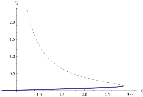
Figure 1: The two roots of eq. (21), $\tilde{\delta}_{a}^{min}$ and $\tilde{\delta}_{a}^{max}$, are shown as function of imaginary frequency $\xi$ (solid and dashed curve respectively). For $\xi\geq 2.85$, $G\leq 0$, at $\xi=2.85$ we have $\tilde{\delta}_{a}^{min}=\tilde{\delta}_{a}^{max}$ and at larger frequency any value of $\tilde{\delta}_{a}$ will give rise to a positive value for (21).

Since $\tilde{\delta}_{a}^{max}$ can be larger than $1$ (see Fig.1) and we assumed $\tilde{\delta}_{a}\ll 1$ we remain with the only possibility $\tilde{\delta}_{a}<\tilde{\delta}_{a}^{min}$. Around $\xi\sim 1$ the condition for the positivity can be written:

$$\tilde{\delta}_{a}<\tilde{\delta}_{a}^{min}=\frac{-E-2\sqrt{E^{2}-4DC}}{2D}\sim-0.0135+0.05148\xi-0.00533\xi^{2}.$$ (22)

If this inequality is satisfied the force density will be repulsive for those values of $\tilde{\delta}_{0}$ which satisfy

$$\tilde{\delta}_{0}^{min}\leq\tilde{\delta}_{0}\leq\tilde{\delta}_{0}^{max},$$ (23)

$\tilde{\delta}_{0}^{min}$ ( $\tilde{\delta}_{0}^{max}$ ) being the smaller (larger) roots of the associated equation:

$$-\tilde{\delta}_{0}^{2}A(\tilde{\delta}_{a},\xi)+\tilde{\delta}_{0}B(\tilde{\delta}_{a},\xi)+C(\tilde{\delta}_{a},\xi) = 0$$ (24)

$$\tilde{\delta}_{0}^{min}=\frac{-B+\sqrt{B^{2}-4AC}}{2A} \sim a_{1}+\tilde{\delta}_{a}a_{2}$$

$$\tilde{\delta}_{0}^{max}=\frac{-B-\sqrt{B^{2}-4AC}}{2A} \sim a_{3}-\frac{1}{\tilde{\delta}_{a}}a_{4}-\tilde{\delta}_{a}a_{2}$$

where

$$a_{1} = 10.48-12.56\xi+4.58\xi^{2},~{}a_{2}=152.438-230.856\xi+93.118\xi^{2},$$

$$a_{3} = -9.16122+12.0305\xi-4.50083\xi^{2},~{}a_{4}=0.376294-0.126549\xi+0.013413\xi^{2}$$

Note that in the case of an ideal mirror at $z=a$ we have $\tilde{\delta}_{a}=0$, $\tilde{\delta}_{0}^{max}\rightarrow\infty$ and the only condition to be satisfied is:

$$\tilde{\delta}_{0}>\tilde{\delta}_{0}^{min}=10.48-12.56\xi+4.58\xi^{2}.$$

Thus the situation in which one mirror is ideal gives rise to quite different results than the ones obtained when both are real. When both mirrors are real, they both must satisfy restrictions to ensure repulsion and, moreover, a precise relation between the two penetration depths must be fulfilled ( eqs. (22,23)).

IV Discussion and Conclusions

Let us apply our results to one known situation, that is of two mirrors described by the plasma model. In this case we have

$$\tilde{\delta}_{(0,a)}=\frac{1}{\sqrt{(\xi^{p}_{(0,a)})^{2}+\xi^{2}}}~{}~{}\text{ with}~{}~{}\xi^{p}_{(0,a)}=a\omega^{p}_{(0,a)}$$

$\omega^{p}_{(0,a)}$ being the plasma frequency of the mirror in $z=(0,a)$ respectively. Condition (22) gives $\xi^{p}_{a}>\frac{1}{0.032}\sim 30.65$ which means that the mirror in $a$ must have a plasma frequency $\omega^{p}_{a}\geq 30.65/a$, but condition (23) implies $\frac{1}{\sqrt{(\xi^{p}_{0})^{2}+1}}>4.37$ which, being $\sqrt{(\xi^{p}_{0})^{2}+1}\geq 1$, is impossible.

Let us consider now the case of hypothetical materials having $\tilde{\delta}_{0}(\xi)=k/\xi$ with $k=1,2,3,4$. There we obtain for the Casimir force, using the exact first three terms of the series eq.(13):

$$a^{4}F_{R}(k=1) = -0.0007-0.0004-0.0000=-0.0011$$

$$a^{4}F_{R}(k=2) = 0.0084-0.0005+0.0000=0.0079$$

$$a^{4}F_{R}(k=3) = 0.0133-0.0006+0.0001=0.0128$$

$$a^{4}F_{R}(k=4) = 0.0164-0.0008+0.0001=0.0157$$

The result is illustrated on Fig. 2. The left hand part shows $\tilde{\delta}_{a}^{min}$ (dashed line) and $\tilde{\delta}_{a}=\frac{1}{\sqrt{30.65^{2}+\xi^{2}}}$ (solid line) as a function of imaginary frequency. In the right hand part the shaded area gives the range of values of $\tilde{\delta}_{0}$ given by condition (23) for which the Casimir force becomes repulsive while the dashed, dotted, dotted-dashed and solid lines, decreasing monotonously with increasing frequency, represent $\tilde{\delta}_{0}$ for $k=1,2,3,4$ respectively. For $k=2,3,4$ the force turns out to be the more repulsive the higher the $k$-value, even though the values of $\tilde{\delta}_{0}$ are only on the limit of the favorable region.

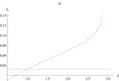
Figure 2: In $a$ $\tilde{\delta}_{a}^{min}$ and $\tilde{\delta}_{a}=\frac{1}{\sqrt{30.65^{2}+\xi^{2}}}$ are shown as dashed and solid curves respectively. In $b$ the area between the two curves $\tilde{\delta}_{0}^{max},\tilde{\delta}_{0}^{min}$ (shaded area) and the curves $k/\xi$ for $k=1,2,3,4$ dashed, dotted, dash-dotted, and thick respectively are shown. For $\xi<1$ $\tilde{\delta}_{a}>\tilde{\delta}_{a}^{min}$ and consequently the results are imaginary and no physical solution exists.

In conclusion we have found sufficient conditions for the Casimir force to be repulsive with an approach considering only the skin depth and needing no specific model of dielectric or magnetic properties. It would be interesting to study now how much these conditions can be softened, as after all to have a positive integral it is not necessary to have a positive integrand. From this point of view our analysis must be deepened trying to obtain analytical necessary conditions for having a repulsive force. Nonetheless our result demonstrate that repulsion is possible if the penetration depth of the two mirrors satisfy appropriate relations.

The approach seems promising as it can be extended to anisotropic material characterized by a tensorial surface impedance and to more general material esqui03 .

It would also be very interesting to derive the skin depth at optical frequencies from the available tabulated data to search for materials matching the conditions we have established and to use our result to design new materials such as to have repulsive properties.

Acknowledgment

Luigi Rosa thanks University of Napoli Federico II for partial financial support and
PRIN Fisica Astroparticellare. He also thanks the Laboratoire Kastler Brossel for the kind hospitality. The authors thank the ESF Research Networking Programme CASIMIR (www.casimir-network.com) for providing excellent opportunities for discussions on the Casimir effect and related topics.

References

(1) H. B. G. Casimir, Proc. Kon. Nederland Akad. Wetensch. B51, 793 (1948).
(2) M. Bordag, U. Mohideen and V.M. Mostepanenko, Phys. Rep. 353, 1 (2001);
K. Milton, J. Phys. A 37, R209 (2004);
V.V. Nesterenko, G. Lambiase, G. Scarpetta, Riv. Nuovo Cimento Ser. 4 27 (6), 1 (2004);
S.K. Lamoreaux, Rept. Prog. Phys. 68, 201 (2005);
F. Capasso, J.N. Munday, D. Iannuzzi, H.B. Chan, IEEE J. Sel. Top. Quant. Electron. 13, 400 (2007).
(3) O. Kenneth, I. Klich, A. Mann, M. Revzen, Phys. Rev. Lett. 89, 033001, (2002).
(4) A. Gusso, A.G.M. Schmidt, Brazilian Journal of Physics 36, 168, (2006).
(6) S.Lee and W.M.Sigmund, J. Coll. Int. Sc., 243, 365 (2001); Coll. Surf. A: Phys. Eng. Asp., 204, 43(2002).
(7) J.N. Mundai, F. Capasso, and A. Parsegian Nature bf 457 170 (2009).
(8)
I. G. Pirozhenko, and A. Lambrecht
J. Phys. A 41, 164015 (2008); I. Pirozhenko, and A. Lambrecht, Phys. Rev. A78, 062102 (2008).
(9) J. A. Stratton,Electromagnetic Theory
(McGraw-Hill, New-York, 1941).
(10) L.D. Landau, and E.M. Lifshits, Electrodynamics of Continuous Media (Oxford, Pergamon, 1984).
(11) V. M. Mostepanenko and N.N. Trunov Sov. J. Nucl. Phys. 4, 818 (1985).
(12) R. Esquivel, C. Villarreal, and W. Luis Mochán,
Phys. Rev. A68 052103 (2003).
(13)
B. Geyer, G. L. Klimchitskaya, and V.M. Mostepanenko, Phys. Rev. A67 062102 (2003).
(14)
N.G. van Kampen, B.R. Nijboer, and K. Schram, Phys. Lett. A 26, 307 (1968).
(15) Yu. S. Barash and V. L. Ginsburg, Usp. Fiz. Nauk 116 5 (1975); Usp. Fiz. Nauk 143 345 (1984);
(16)
T. H. Boyer, Phys. Rev. A 9, 2078 (1974).
(17)
C. Henkel and K. Joulain, Europhys. Lett. 72, 929 (2005).
(18) A. Romeo, and A. Saharian, J. Phys. A 35, 1297,(2002).
(19) M. Abramowitz, and I.A. Stegun Handbook of Mathematical Functions (National Bureau of Standards Applied Mathematics Series 55, Washington D.C., 1972).