Dynamic Screening and Low Energy Collective Modes in Bilayer Graphene

Abstract

We theoretically study the dynamic screening properties of bilayer graphene within the random phase approximation assuming quadratic band dispersion and zero gap for the single-particle spectrum. We calculate the frequency dependent dielectric function of the system and obtain the low energy plasmon dispersion and broadening of the plasmon modes from the dielectric function. We also calculate the optical spectral weight (i.e. the dynamical structure factor) for the system. We find that the leading order long wavelength limit of the plasmon dispersion matches with the classical result for 2D electron gas. However, contrary to electron gas systems, the non-local plasmon dispersion corrections decrease the plasmon frequency. The non-local corrections are also different from the single layer graphene. Finally, we also compare our results with the double layer graphene system (i.e. a system of two independent graphene monolayers).

I Introduction

Bilayer graphene (BLG) has recently attracted experimental and theoretical interest, both for fundamental physics as well as for possible technological applications blg1 ; blg2 ; hwang:rossi ; blgtransport:expt ; optics:expt ; slgreview . The system consists of two layers, each of which has carbon atoms arranged in a honeycomb lattice with two (A and B) sublattices. Each layer can be viewed as a single layer graphene (SLG) slgreview with their associated physics of chiral Dirac Fermions, coupled by strong interlayer tunneling between A and B lattice sites in the two layers. It is useful to view BLG as an effective layer where the interlayer tunneling changes the linear dispersion of the quasiparticles in SLG to an effective quadratic dispersion at small wavevectors blg2 . Thus, a simple model for BLG single-particle spectrum is a pair of chiral parabolic electron and hole bands touching each other at the Dirac (or the charge neutrality) point. Each band has a 4-fold degeneracy arising from spin and valley degrees of freedom. The pristine or undoped bilayer graphene has attracted a lot of interest since the presence of a single Fermi point and quadratic dispersion can lead to a host of exotic phenomena kunyang1 ; levitov1 . The low energy properties of the doped bilayer graphene also show interesting features like enhanced backscattering due to the chirality of the bands present in the system hwang:blgstatic . The single-particle spectrum is sufficiently different in SLG (linear dispersions) and BLG (quadratic dispersions) that it is theoretically interesting to explore and contrast various dielectric properties in the two systems. In this paper we consider the dynamic screening and low energy collective modes of BLG.

Coulomb interaction and its dynamic screening due to many-body effects is an important property of any electronic material. While static screening determines transport properties, the dynamic (frequency dependent) screening determines the elementary quasiparticle spectra and the collective modes and is crucial to understanding the optical properties of the system. While much work has been done on screening properties and plasmon modes of SLG both theoretically hwang:slgdynamic and experimentally slgexpt , there are very few existing analytic works on doped bilayer systems. There are numerical calculations of the bilayer dynamic screening within a four-band model macdonald , and the parabolic approximation chakravorty1 ; chakravorty2 , but it is not useful in a general context. Ref. chakravorty2, obtains results which are qualitatively similar to the results in this paper. Recently, the static screening properties of BLG systems have been studied analytically in Ref. hwang:blgstatic, . In this paper, we will analytically study the dynamic screening of Coulomb interactions in doped BLG and obtain its collective modes.

The parabolic dispersion makes the BLG low energy physics quite different from SLG systems. On the other hand, although the system has the same low energy dispersion as a regular two dimensional electron gas (2DEG) system, the chirality of graphene leads to features which are distinct from a standard 2DEG 2DEG which has been extensively studied in the context of semiconductor heterostructures semiconductor . It is therefore useful to compare the physics of BLG with SLG and 2DEG. In this respect, it is important to note that although bilayer graphene consists of two layers of graphene sheets, it should really be viewed as a 2D system with parabolic dispersion and chiral bands for the purpose of low energy physics. Thus, it is also important to compare this system with other bilayer systems such as double quantum wells Madhukar ; Hwang:tunnel , which consists of two layers of 2DEG coupled by Coulomb interaction and shows distinct features as a result of its quasi-2D nature. Another closely related system is the double layer graphene, which is obtained by putting a layer of oxide between two single layers of graphenedlg:expt . In this case, the layer separation is much larger ($\sim 10nm$) than in BLG ($\sim 0.3nm$) and the system is better viewed as two different layers of graphene coupled by Coulomb interactions without any interlayer tunneling. The dynamic screening properties of BLG is quite different from these systems. It is then useful to compare the results obtained for BLG with corresponding results in these two bilayer systems (i.e. two layers of 2DEG and two layers of SLG).

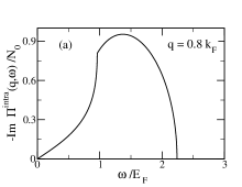
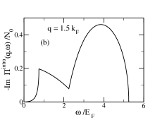
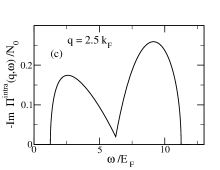
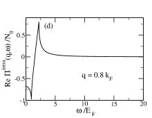
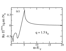
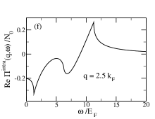
Figure 1: (a)-(c): Imaginary part of Intraband susceptibility as a function of frequency for (a) $q=0.8k_{F}$ (b) $q=1.5k_{F}$ and (c) $q=2.5k_{F}$. (d)-(f): Real part of Intraband susceptibility as a function of frequency for (d) $q=0.8k_{F}$ (e) $q=1.5k_{F}$ and (f) $q=2.5k_{F}$.

In this paper, we analytically study the dynamic screening properties of the Coulomb interaction in BLG systems within the random phase approximation (RPA). We calculate the dielectric function of bilayer graphene, $\epsilon({\bf q},\omega)$ at arbitrary wavevectors ${\bf q}$ and frequency $\omega$. The imaginary part of $1/\epsilon({\bf q},\omega)$ is related to the optical spectral weight which can be directly measured in optical conductivity li2008 or light-scattering lightscatter , or electron-scattering measurements slgexpt ; ieel while the zeroes of the real part give the dispersion of the plasmon modes. We calculate the plasmon modes and their damping due to the presence of the second band in the system. We make extensive comparisons of our results with similar results for SLG systems hwang:slgdynamic and 2DEG 2DEG , especially regarding the dependence of collective mode dispersions on the carrier densities in these systems. We look at the density dependence of the long wavelength collective mode dispersion and show how the system crosses over from a BLG like behaviour to a SLG like behaviour as density of the carriers is increased. We also compare our results with those for quasi-2D systems like double quantum wells Madhukar and double layer graphene hwang:dlg and show that in spite of having two layers, bilayer graphene shows unique features in its dynamic screening properties.

We note that we are working here with the parabolic approximation to the dispersion of the BLG bands. In real bilayer systems, the dispersion changes from parabolic to a linear form (i.e. the full dispersion is hyperbolic) at high energies. In addition the 2 band approximation breaks down at higher energies, resulting in a 4-band BLG model. However, it is clear that for low density materials, the low energy properties of the system are qualitatively well described by keeping only the parabolic part of the dispersion. For bilayer graphene systems, our parabolic approximation for collective modes should be valid upto densities $\sim 5\times 10^{12}cm^{-2}$.

Our BLG model, as mentioned above, consists of a 2-band (single valence and conduction band) gapless parabolic chiral 2D single-particle energy dispersion. We compare our analytic dynamic screening and collective mode BLG results with SLG (chiral gapless 2-band linear dispersion), 2DEG (non-chiral 1-band gapped parabolic dispersion), double-layer graphene (two parallel SLG) and 2D bilayer ( two parallel 2DEG) systems. Our theoretical results, therefore, give a fairly complete picture of dielectric screening and plasmon modes in 2D systems, covering both single and bilayer systems, both linear and quadratic band dispersions, system with and without gaps, and both chiral and non-chiral situations. Our calculated BLG plasmon dispersion can be directly compared with experimental results when they become available.

The low energy effective Hamiltonian for BLG is given by

$$H=-\frac{1}{2m}\left(\begin{array}[]{cc}0&(k_{x}-ik_{y})^{2}\\ (k_{x}+ik_{y})^{2}&0\end{array}\right),$$ (1)

where $m=\gamma/(2v_{F}^{2})$ , $\gamma$ is the interlayer tunneling amplitude inherent in the BLG system and $v_{F}$ is the graphene Fermi velocity. We set $\hbar=1$ throughout this paper. Typically, in the BLG systems $m\simeq 0.033m_{0}$, with $m_{0}$ being the free electron mass. This Hamiltonian differs from the SLG case in having a quadratic as opposed to a linear dispersion. As a result, the system has a constant density of states rather than the linear density of states in SLG. As we will see, this leads to substantial difference in the BLG dielectric response.

The Hamiltonian can be diagonalized to obtain two bands with dispersions $\epsilon^{s}_{\bf k}=s{\bf k}^{2}/(2m)$ and corresponding wavefunctions $\Psi^{s}_{\bf k}=\frac{e^{i{\bf k}\cdot{\bf r}}}{\sqrt{2}}\left(e^{-2i\chi_{\bf k}},s\right)$, where $s=\pm 1$ denotes respectively the conduction and the valence band. Here $\chi_{\bf k}=\tan^{-1}(k_{y}/k_{x})$. In this paper we use the parabolic Hamiltonian to obtain the dynamic screening within random phase approximation (RPA). This involves a theoretical calculation of the dynamical dielectric function $\epsilon({\bf q},\omega)$.

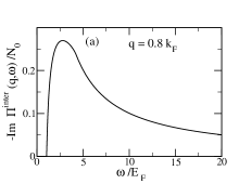
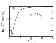
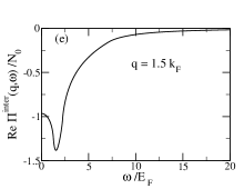
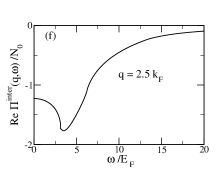
Figure 2: (a)-(c): Imaginary part of Interband susceptibility as a function of frequency for (a) $q=0.8k_{F}$ (b) $q=1.5k_{F}$ and (c) $q=2.5k_{F}$. (d)-(f): Real part of Interband susceptibility as a function of frequency for (d) $q=0.8k_{F}$ (e) $q=1.5k_{F}$ and (f) $q=2.5k_{F}$.

II Bare Bubble Polarizability

The frequency dependent dielectric function for this system (within RPA) is given by

$$\epsilon({\bf q},\omega)=1-\frac{2\pi e^{2}}{\kappa q}\Pi({\bf q},\omega),$$ (2)

where $\kappa$ is the background dielectric constant. Here $\Pi$ is the free particle (bare bubble) polarizability, given by

$$\Pi({\bf q},\omega)=g\sum_{ss^{\prime}{\bf k}}\frac{f^{s}_{\bf k}-f^{s^{\prime}}_{{\bf k}+{\bf q}}}{\omega+\epsilon^{s}_{\bf k}-\epsilon^{s^{\prime}}_{{\bf k}+{\bf q}}}F_{ss^{\prime}}({\bf k},{\bf k}+{\bf q}),$$ (3)

where $f^{s}_{\bf k}$ is the Fermi function, $g$ is the degeneracy factor ($g=4$) and the wavefunction overlap $F_{ss^{\prime}}({\bf k},{\bf k}+{\bf q})=\frac{1}{2}[1+ss^{\prime}\cos(2\theta)]$ with $\theta$ being the angle between ${\bf k}$ and ${\bf k}+{\bf q}$. Using a circular co-ordinate system $(k,\phi)$, one can write $\cos\theta=(k+q\cos\phi)/|{\bf k}+{\bf q}|$. The chirality effect is incorporated in the matrix element $F$.

The polarizability can be separated into the intraband ($s=s^{\prime}$ terms) and the interband ($s^{\prime}=-s$ terms) contributions. The scale for the polarizability is set by the free particle density of states $N_{0}=gm/(2\pi)$. Using the Fermi momentum $k_{F}^{-1}$ and the Fermi energy $E_{F}$ as units of length and energy respectively, we work with the dimensionless variables $x=k/k_{F}$, $y=q/k_{F}$ and $z=\omega/E_{F}$. Then, we can write $\Pi(q,\omega)=N_{0}[\Pi^{inter}(y,z)+\Pi^{intra}(y,z)]$, where $\Pi^{intra}$and $\Pi^{inter}$ are dimensionless quantities. Note that the interband contribution is important in graphene only because of its gapless nature; in semiconductor based 2DEG, the interband contribution is implicitly included in the background dielectric constant and is not considered in the electronic polarizability.

We consider a gated or doped BLG with $E_{F}\neq 0$, where the Fermi level lies in the conduction band. At $T=0$, this implies that $f^{+}_{\bf k}=\Theta(k_{F}-k)$ and $f^{-}_{\bf k}=1$. Then one can write $\Pi^{intra}(y,z)=\Pi^{1}(y,z)+\Pi^{1}(-y,-z)$, where

$$\displaystyle\Pi^{1}(y,z) = \frac{1}{\pi}\int_{0}^{1}xdx\displaystyle{\int_{-\pi}^{\pi}}d\phi\frac{1}{z-y^{2}-2xy\cos\phi}$$ (4)

$$~{}~{}~{}~{}~{}~{}~{}~{}~{}~{}\left[1-\frac{y^{2}\sin^{2}\phi}{x^{2}+y^{2}+2xy\cos\phi}\right],$$

and $\Pi^{inter}(y,z)=\Pi^{2}(y,z)+\Pi^{2}(-y,-z)$, where

$$\displaystyle\Pi^{2}(y,z) = \frac{-1}{\pi}\int_{1}^{\infty}xdx\displaystyle{\int_{-\pi}^{\pi}}d\phi\frac{\sin^{2}\phi}{x^{2}+y^{2}+2xy\cos\phi}$$ (5)

$$~{}~{}~{}~{}~{}~{}~{}~{}~{}~{}~{}~{}\frac{y^{2}}{z+2x^{2}+y^{2}+2xy\cos\phi}.$$

The azimuthal integrals in eqns. (4) and (5) can be done analytically to obtain

$$\Pi^{1}(y,z) = \frac{-1}{2}\displaystyle\int_{0}^{1}\frac{dx}{x(x^{2}+z)}\left[x^{2}+z-|x^{2}-y^{2}|\right.$$

$$- \left.Sgn[z-y^{2}+2xy]\frac{(2x^{2}+z-y^{2})^{2}}{\sqrt{(z-y^{2})^{2}-4x^{2}y^{2}}}\right],$$

$$\Pi^{2}(y,z) = \frac{1}{2}\displaystyle\int_{1}^{\infty}\frac{dx}{x(x^{2}+z)}\left[x^{2}+z+|x^{2}-y^{2}|\right.$$

$$- Sgn[(x-y)^{2}+x^{2}+z]$$

$$\left.~{}~{}~{}\sqrt{(2x^{2}+z+y^{2})^{2}-4x^{2}y^{2}}\right],$$

where $Sgn(x)=\pm 1$, depending on $x\gtrless 0$. The real and imaginary parts of the polarizability are even and odd under $z\rightarrow-z$; so we will only consider the case of $z>0$. The real and imaginary parts of the intraband polarizability are

$$\text{Re}~{}\Pi^{intra}(y,z) = f_{1}(y,z)+f_{1}(y,-z)$$ (8)

$$- \Theta[(z-y^{2})^{2}-4y^{2}]f_{2}(y,z)$$

$$- \Theta[(z+y^{2})^{2}-4y^{2}]f_{2}(y,-z),$$

$$\text{Im}~{}\Pi^{intra}(y,z) = -\Theta[4y^{2}-(z-y^{2})^{2}]f_{3}(y,z)$$ (9)

$$+ \Theta[4y^{2}-(z+y^{2})^{2}]f_{3}(y,-z).$$

For notational brevity, it is useful to define the quantities $a=(z-y^{2})/2y$ and $b=(z+y^{2})/2y$. Then we have

$$f_{1}(y,z) = \frac{ya}{2z}\log\left|\frac{4y^{2}a^{2}}{1-z}\right|-\frac{1}{2}$$ (10)

$$+ \frac{ya}{z}\Theta[1-y]\log\left|\frac{1-z}{2ya}\right|,$$

$$f_{2}(y,z) = Sgn[a]\left[\frac{\sqrt{a^{2}-1}}{y}+\frac{yb}{2z}\log\left|\frac{\sqrt{a^{2}-1}-b}{\sqrt{a^{2}-1}+b}\right|\right.$$ (11)

$$- \left.\frac{ya}{2z}\log\left|\frac{\sqrt{a^{2}-1}-a}{\sqrt{a^{2}-1}+a}\right|\right],$$

$$f_{3}(y,z) = \frac{\sqrt{1-a^{2}}}{y}+\frac{y|a|}{z}\tan^{-1}\left[\frac{\sqrt{1-a^{2}}}{|a|}\right]$$ (12)

$$- \frac{y|b|}{z}\tan^{-1}\left[\frac{\sqrt{1-a^{2}}}{|b|}\right].$$

For the interband polarizability, it is useful to define: $c=y\sqrt{y^{2}+2z}$ and $d=y\sqrt{2z-y^{2}}$. Then we can write

$$\text{Re}~{}\Pi^{inter}(y,z)= f_{4}(y,z)+f_{4}(y,-z)+f_{5}(y,z)$$ (13)

$$+ \Theta[(z-2)^{2}+d^{2}]Sgn(2-z-|d|)f_{5}(y,-z)$$

$$\text{Im}~{}\Pi^{inter}(y,z) = \Theta[2z-y^{2}]\Theta[z-2+d]$$ (14)

$$\left[\Theta[z-2-d]\frac{\pi}{2}\left(\frac{|z-y^{2}|}{z}-1\right)\right.$$

$$\left.+\Theta[2+d-z]f_{6}(y,z)\right]$$

where

$$f_{4}(y,z) = \frac{1}{2}\left[\log\left|\frac{c}{4}\right|-\frac{z+y^{2}}{2z}\log|1+z|\right.$$

$$- \left.\frac{\sqrt{c^{2}+z^{2}}}{2z}\log\left|\frac{\sqrt{c^{2}+z^{2}}-z}{\sqrt{c^{2}+z^{2}}+z}\right|\right.$$

$$+ \left.\Theta[y-1]\frac{z+y^{2}}{2z}\log\left|\frac{1+z}{z+y^{2}}\right|\right]$$

$$f_{5}(y,z) = \frac{1}{2}\left[\log\left|\frac{2+z+\sqrt{(2+z)^{2}+c^{2}}}{c}\right|+\frac{\sqrt{c^{2}+z^{2}}}{2z}\right.$$ (16)

$$\left.\log\left|\frac{\sqrt{c^{2}+z^{2}}(2+z)-z\sqrt{(2+z)^{2}+c^{2}}}{\sqrt{c^{2}+z^{2}}(2+z)+z\sqrt{(2+z)^{2}+c^{2}}}\right|\right]$$

$$f_{6}(y,z) = \frac{|z-y^{2}|}{2z}\left[\frac{\pi}{2}-\tan^{-1}\left(\frac{|z-y^{2}|(2-z)}{z\sqrt{d^{2}-(2-z)^{2}}}\right)\right]$$ (17)

$$-\frac{1}{2}\left[\frac{\pi}{2}-\sin^{-1}\left(\frac{2-z}{d}\right)\right]$$

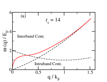
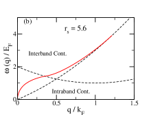
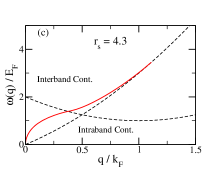
Figure 3: Optical plasmon dispersion in bilayer graphene systems for (a) $r_{s}=14$ (b) $r_{s}=5.6$ and (c) $r_{s}=4.3$. The thick red line is the plasmon dispersion, while the dashed lines show the upper edge of the intraband continuum and the lower edge of the interband continuum. (color online).

Eqn.s (8-17) are the main analytic results of this paper. These equations completely define the BLG RPA dynamic response (and consequently the collective plasmon modes) analytically within the 2-band low energy quadratic band dispersion approximation. We first point out the essential features of the polarizability which differentiate it from the 2DEG and SLG systems.

The intraband polarizability has an imaginary part for $0<z<y^{2}+2y$ for $y<2$ and for $y^{2}-2y<z<y^{2}+2y$ for $y>2$, which defines the band of particle-hole continuum. For $y<1$, there is a discontinuity in the derivative at $z=2y-y^{2}$, which is qualitatively similar to the 2DEG results. For $2>y>1$, an additional derivative discontinuity appears at $z=y^{2}$, which is a result of the chiral nature of the wavefunctions. For $y>2$, the feature at $z=y^{2}$ persists, while $z=2y-y^{2}$ shifts to the lower edge of the particle-hole continuum. These features are shown in Fig. 1(a), (b) and (c) respectively. These features result in sharp features in the real part of the polarizability. However, unlike SLG systems, the polarizability does not diverge at the upper edge of the continuum. The singularity in this case is softened to a derivative discontinuity. The real part of the polarizability for different wavevectors is plotted in Fig. 1 (d), (e) and (f) respectively.

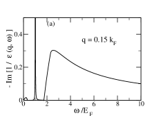
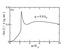
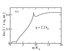
Figure 4: Imaginary part of inverse dielectric function for (a) $q=0.15k_{F}$ (undamped plasmon), (b) $q=0.8k_{F}$ (damped plasmon) and (c) $q=2.2k_{F}$ (no plasmon pole). All figures are for $r_{s}=4.3$.

The imaginary part of the interband polarizability is non-zero for $z>y^{2}-2y+2$ for $y<2$ and for $z>y^{2}/2$ for $y>2$ which defines the interband continuum. For $z>y^{2}+2y+2$, it has the simple form $\sim y^{2}/z$. For $y>1$, there is a derivative discontinuity at $z=y^{2}$. The real part of the polarizability shows a peak at the lower edge of the interparticle continuum. The imaginary and real part of the interband polarizability are plotted in Fig. 2(a), (b), (c) and Fig. 2 (d), (e) and (f) respectively.

III Plasmons and Optical Spectral weight

The dielectric function can be used to calculate the dispersion and damping of plasmons, which are the long-wavelength longitudinal collective modes of the density fluctuations. The dispersion can be obtained by looking for poles of the two-particle Green functions or equivalently for zeroes of the real part of the dynamical dielectric function. It is useful to express the dielectric function in terms of the dimensionless quantities $y=q/k_{F}$ and $z=\omega/E_{F}$.

$$\epsilon({\bf q},\omega)=1-\frac{r_{s}}{y}(\Pi^{intra}(y,z)+\Pi^{inter}(y,z)),$$ (18)

where the dimensionless ratio $r_{s}=e^{2}gm/(\kappa k_{F})$ denotes the ratio of the interaction energy scale to the kinetic energy scale in the system. It is important to note that unlike SLG systems, where $r_{s}$ is only a function of the substrate dielectric constant and can take a few discrete values, $r_{s}$ for BLG systems can be varied continuously by changing the gate voltages and hence density of the carriers. The coupling constant $r_{s}$ in BLG is thus similar to that in 2DEG with carrier density being the tuning parameter ($r_{s}\sim n^{-1/2}$).

There are two collective modes of this system, an optical plasmon mode which lies above the intraband electron-hole continuum and an acoustic plasmon mode which lies within the intraband continuum. The acoustic mode, which has a linear dispersion at long wavelength limit is always overdamped. Thus it carries very little spectral weight and is not experimentally relevant. In the following we will focus on the optical plasmon mode (henceforth referred to as the plasmon).

To get the dispersion of the optical plasmon, we note that the mode lies between the intraband and interband continuum in the low wavelength limit. In this limit we can expand the polarizability to obtain

$$\Pi(y,z)=2\frac{y^{2}}{z^{2}}-\frac{y^{2}}{4}.$$ (19)

In the long wavelength limit, we find that the plasmon has a leading order $\sim\sqrt{q}$ dispersion. In this limit, we recover the 2DEG result in leading order in $q$

$$\omega_{q}\simeq e\sqrt{\frac{gE_{F}}{\kappa}}\sqrt{q}.$$ (20)

Expanding to next order, we can obtain the quantum (non-local) corrections to the plasmon dispersion. The BLG plasmon dispersion is upto this order is given by

$$\omega_{q}\simeq e\sqrt{\frac{gE_{F}q}{\kappa}}\left(1-\frac{q_{TF}q}{8k_{F}^{2}}\right).$$ (21)

where $q_{TF}=r_{s}k_{F}$ is independent of the density.

We next compare the plasmon dispersion for BLG systems with those of SLG and a 2DEG. For the sake of comparison, we first note that the plasmon dispersion formulae for both SLG hwang:slgdynamic and 2DEG 2DEG can be cast in a form similar to BLG, $\omega_{q}=\omega_{0}q^{1/2}(1-\alpha q/k_{f}^{2})$. We first focus on the leading order $\sim\sqrt{q}$ term. For BLG , the coefficient of the leading order term is given by $\omega_{0}=(ge^{2}E_{F}/\kappa)^{1/2}$, while for SLG it is given by $\omega_{0}=(ge^{2}v_{F}k_{F}/2\kappa)^{1/2}$. For the 2DEG it is given by $\omega_{0}=(ge^{2}E_{F}/\kappa)^{1/2}$. The density dependence ($\sim n^{1/2}$) of $\omega_{0}$ in BLG is different from that of SLG hwang:slgdynamic ($\sim n^{1/4}$), and is a consequence of a constant as opposed to a linear density of states. The long wavelength BLG plasmon is thus identical to the ordinary 2D plasmon and is thus different from the long wavelength SLG plasmon. In particular, the long wavelength BLG plasma frequency, in contrast to the SLG plasma frequency dassarma2009 , is classical and does not have any $\hbar$ in the leading order dispersion.

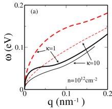
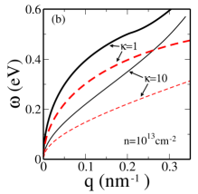
Figure 5: Plasmon frequency for BLG (solid black) and SLG (dashed red) systems for two different values of substrate dielectric constant $\kappa=1$ and $\kappa=10$. The two figures are for different densities (a) $n=10^{12}cm^{-1}$ and (b) $n=10^{13}cm^{-1}$ (color online).

However, the difference with the 2DEG result occurs in the next order which encapsulates the effect of the quantum corrections. For the BLG plasmon, $\alpha=q_{TF}/8$ with $q_{TF}=r_{s}k_{F}$ being independent of density. For the 2DEG, $\alpha=-3q_{TF}/4$ with $q_{TF}=gme^{2}/\kappa$. Thus, the quantum corrections increase the plasmon frequency from its leading order result in 2DEG, while in BLG they lead to a reduction of the plasmon frequency. For SLG, $\alpha=q_{TF}/8$ with $q_{TF}=ge^{2}k_{F}/v_{F}\kappa\sim n^{1/2}$. The quantum corrections thus decrease the SLG plasmon frequency. However the density dependence of this correction term is very different from the BLG case.

The other major difference from the single layer graphene is that in SLG systems, there is a singularity of the real part of the polarizability at the upper edge of the intraband continuum. Hence, the plasmon dispersion never goes into the continuum and the pole survives upto arbitrary large wave-vectors. In bilayer systems, there is no discontinuity at the upper edge of the intraband continuum (it is replaced by a discontinuity in the derivative with respect to frequency), and so, at a critical wave-vector, the plasmon pole vanishes once the plasmon dispersion touches the edge of the continuum.

In order to compare BLG and SLG plasmon dispersions we plot in Fig. 5 the plasmon dispersion (in absolute units of eV) as a function of wavevector (in absolute units of $nm^{-1}$) for two fixed density of careers (a) $n=10^{12}cm^{-1}$ and (b) $n=10^{13}cm^{-1}$ . For each value of density we plot the plasmon dispersion for two values of $\kappa=1$ and $\kappa=10$. We see that the BLG plasmon merges with the intraband continuum at a finite wavevector and gets overdamped while the SLG plasmon is present at all wavevectors. At the lower density the SLG plasmon frequency is higher than the BLG plasmon while at the higher density the BLG plasmon has a higher frequency than SLG plasmon as $\omega_{0}\propto\sqrt{E_{F}}$ and the Fermi energy has different dependence on density in the two cases.

At long wavelengths, the plasmon mode is completely undamped. As the dispersion goes into the interband continuum at larger wavevectors, two things happen: (i) the mode gets damped due to usual Landau damping by the particle-hole pairs, and (ii) the dispersion develops a knee like structure due to mode repulsion from the continuum.

In order to look at typical BLG plasmon dispersions, we consider three types of substrates: (a) $SiC$, which has $\kappa=5.5$, (b) $SiO_{2}$, which has $\kappa=4$ and (c) vacuum, corresponding to suspended bilayer graphene, with $\kappa=1$. Note that the effective $\kappa$ to be used for calculation of $r_{s}$ is the average of $\kappa$ for the substrate and that for the vacuum. For a typical density of $10^{12}cm^{-2}$, we get $r_{s}\sim 4.3$ for $SiC$, $r_{s}=5.6$ for $SiO_{2}$ and $r_{s}=14$ for suspended bilayer graphene. The plasmon dispersion for these three values of $r_{s}$ are shown in Fig. 3. The critical wavevector for plasmon damping does not change much varying from $q_{1}=0.29k_{F}$ for $r_{s}=14$ to $q_{1}=0.38k_{F}$ for $r_{s}=4.3$. The maximum wavevector for which the plasmon pole exists varies from $q_{max}=1.12k_{F}$ for $r_{s}=4.3$ to $q_{max}=1.52k_{F}$ for $r_{s}=14$.

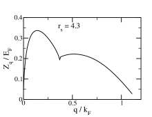
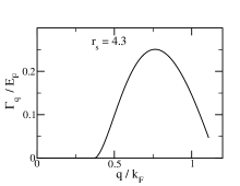
Figure 6: (a) The quasiparticle residue $Z$ and (b) The width $\Gamma$ of the plasmon pole in the inverse dielectric function for $r_{s}=4.3$.

An important quantity which is directly measured in spectroscopic experiments is the optical spectral weight or the loss function. This quantity is proportional to the imaginary part of the inverse dielectric function of the system. In Fig. 4, we plot the spectral weight for three different wavevectors for $r_{s}=4.3$. The first wavevector ($q=0.15k_{F}$) corresponds to the situation where the plasmon mode lies between the intraband and interband continuum. The plasmon in this case is sharp, i.e. not Landau-damped. The second wavevector ($q=0.8k_{F}$) corresponds to the situation where the plasmon peak has entered into the interband continuum. In this case we see a broadened plasmon peak. The third wavevector ($q=2.2k_{F}$) corresponds to the case where the plasmon pole has vanished, and the collective mode is overdamped. It is to be noted that since the dielectric function continues to have a kink at the edge of the intraband continuum even when the plasmon has ceased to exist, a peak like structure is seen in the optical spectral weight in this limit. This peak vanishes at much larger wavevectors $\sim 4k_{F}$ for $r_{s}=4.3$.

Focusing on the plasmons, one can expand the inverse dielectric function near the plasmon pole to write

$$\frac{1}{\epsilon({\bf q},\omega)}=\frac{Z_{q}}{\omega-\omega_{q}+i\Gamma_{q}}.$$ (22)

where the $\omega_{q}$ is the plasmon frequency, $Z_{q}=-1/[V(q)\partial\Pi^{{}^{\prime}}(q,\omega)/\partial\omega|_{\omega=\omega_{q}}]$ is the plasmon pole residue or equivalently, the weight of the plasmon peak, and the width of the peak is given by $\Gamma_{q}=-V(q)\Pi^{{}^{\prime\prime}}(q,\omega_{q})Z_{q}$. Here $\Pi^{{}^{\prime}}$ and $\Pi^{{}^{\prime\prime}}$ denote the real and imaginary part of the polarizability. In Fig. 6 we plot $Z_{q}$ and $\Gamma_{q}$ as a function of $q$ for $r_{s}=4.3$.

The plasmon weight $Z_{q}\sim\sqrt{q}$ in the long wavelength limit. It shows a broad peak before the plasmon dispersion enters the interband continuum. At the lower edge of the interband continuum, $Z_{q}$ shows a kink as a function of $q$. It flattens out over a substantial range of wavevectors before finally going to zero as the plasmon approaches the intraband continuum and vanishes. The width of the plasmon peak starts from zero at the interband edge and shows a broad feature before going to zero again as the plasmon vanishes. The plasmon features predicted in our theory (Figs.  3- 6) should be directly observable in inelastic electron energy loss (IEEL) slgexpt ; ieel or inelastic light scattering (ILS) spectroscopies lightscatter where the loss function can be mapped out as a function of ${\bf q}$ and $\omega$.

IV Hyperbolic dispersion and Crossover from BLG to SLG physics

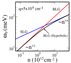
Figure 7: The scaling of the leading order plasmon dispersion in the long wavelength limit with density on a log-log scale. The leading order result is obtained by evaluating the plasmon dispersion at a wavevector $q=5\times 10^{4}cm^{-1}$. The red line is the BLG result with parabolic dispersion. The blue line is the SLG result. The black line is the BLG plasmon dispersion with hyperbolic dispersion (color online).

We have treated bilayer graphene as a system with quadratic band dispersion and chiral electron and hole bands. While the parabolic dispersion is relevant at low energies, the actual dispersion of the bands is hyperbolic. Thus at large wavevectors (relevant at large densities) the dispersion is effectively linear and the system should behave like single layer graphene, while at small wavevectors (relevant at low densities) it should behave like the bilayer graphene system we have described. In this section, we wish to study this crossover by focusing on the long-wavelength limit of the plasmon dispersion. Although the full plasmon dispersion at all wavevectors can be obtained numerically, working with the leading order long wavelength dispersion lets us obtain analytic results and hence provides insight into the crossover. This will also let us estimate the regime of validity of our parabolic band approximation.

To estimate the long wavelength plasmon, we note that for $qv_{F}/\omega\ll 1$, the bare bubble polarizability is given by

$$\Pi({\bf q},\omega)=\frac{gk_{F}}{4\pi}\frac{q^{2}}{\omega^{2}}\left.\frac{\partial E_{\bf k}}{\partial_{\bf k}}\right|_{k=k_{F}}$$ (23)

where $E_{\bf k}$ is the dispersion of the band containing the Fermi level. Hence the long wavelength plasmon dispersion is given by

$$\omega_{q}^{2}=\frac{ge^{2}k_{F}q}{2\kappa}\frac{dE_{F}}{dk_{F}}=\frac{ge^{2}n}{\kappa}\frac{dE_{F}}{dn}q$$ (24)

where $n$ is the density of carriers and we have used $n=gk_{F}^{2}/(4\pi)$. The above results are true for any dispersion including (a) a parabolic dispersion, (b) a linear dispersion and (c) a hyperbolic dispersion. Let us now focus on the hyperbolic dispersion of BLG. In this case one can write the Fermi energy as a function of density as slgreview

$$E_{F}=\left[\frac{\gamma^{2}}{2}+\frac{4\pi v_{F}^{2}}{g}n-\frac{\gamma^{2}}{2}\sqrt{1+\frac{16\pi v_{F}^{2}n}{g\gamma^{2}}}\right]^{1/2}$$ (25)

where $\gamma$ is the interlayer tunneling and $v_{F}$ is the Fermi velocity of the graphene sheets. Note that in the limit of small $n\rightarrow 0$, $E_{F}\sim k_{F}^{2}/2m$ with $m=\gamma/(2v_{F}^{2})$ and we recover the parabolic Fermi energy, while in the large density limit ($n\rightarrow\infty$), $E_{F}=v_{F}k_{F}$ and we recover the single layer graphene results. Now the long wavelength plasmon frequency for hyperbolic dispersion is then given by

$$\omega_{q}^{2}=\frac{2\pi ne^{2}}{\kappa}\frac{v_{F}^{2}}{E_{F}}q\left[1-\frac{1}{\sqrt{1+\frac{16\pi v_{F}^{2}n}{g\gamma^{2}}}}\right]$$ (26)

In the low density limit ($n\rightarrow 0$) this reduces to $\omega_{\bf q}^{2}=(2\pi ne^{2})q/(\kappa m)$ and we recover the leading order result for the bilayer graphene with parabolic dispersion. In the large density limit ($n\rightarrow\infty$), the limiting behaviour is given by $\omega_{\bf q}^{2}=e^{2}v_{F}\sqrt{g\pi n}q/\kappa$ which matches with the result for single layer graphene hwang:slgdynamic . In between the answer smoothly interpolates between these two limits.

In Fig. 7 we plot the plasmon frequency at a low wavevector ($q=5\times 10^{4}cm^{-1}$) as a function of density on a log-log scale. The low wavevector ensures that we are looking at the leading order result. We plot the results for BLG and SLG which show the usual $n^{1/2}$ and $n^{1/4}$ scaling respectively. The curve for hyperbolic dispersion of BLG smoothly interpolates between the above two curves. From the figure we can estimate the value of critical career density where the hyperbolic result differs significantly from the parabolic result. By comparing the long wavelenght plasma frequencies in SLG and BLG we obtain the crossover density as $n_{c}=m^{2}v_{F}^{2}/\pi$. This correspond to a density $n\sim 3\times 10^{12}cm^{-1}$ for a bilayer effective mass $m\simeq 0.033m_{e}$ (see Fig. 7). This then gives us the limit of validity of the parabolic approximation for BLG systems.

V Comparison with Other Bilayer Systems

Figure 8: Low energy plasmon dispersion for three different bilayer systems: (a) an n-GaAs double quantum well with $r_{s}=1$ (corresponding to a density of $n=3.2\times 10^{11}cm^{-2}$ and a layer separation of $d=9.5nm$, which corresponds to the effective Bohr radius of n-GaAs quantum well) (b) a double layer graphene with a density of $n=10^{12}cm^{-2}$ and a layer separation of $d=3\AA$ (which corresponds to the layer separation of bilayer graphene) and (c) a bilayer graphene system with a density of $n=10^{12}cm^{-2}$ and $r_{s}=4.3$. The $sqrt{q}$ mode is in blue and the linear mode is in red solid lines. The black lines indicate interband and intraband continuum. The undamped linear acoustic mode is absent in bilayer graphene ( color online).

The study of dielectric functions and plasmons for bilayer systems have a long history starting with the prediction of an undamped acoustic plasmon mode in double quantum wells Madhukar with layer separation greater than a critical distance. Similar results have also been obtained for double layer graphene systems hwang:dlg . However, the physics of these systems is quite different from the bilayer graphene system which is of interest in this paper. These other systems are comprised of well separated 2D layers coupled only by the Coulomb interaction. Interlayer tunneling is absent in these systems. On the other hand, the bilayer graphene system is in the opposite limit of small layer separation with layers coupled strongly through interlayer tunneling, which is accounted for in the model by changing the low energy dispersion from linear to quadratic. This leads to all the major differences between the bilayer graphene and other double layer systems.

The double layer 2DEG systems in the limit of infinite separation corresponds to two copies of the underlying 2D systems. Hence it has two plasmon modes (one in each layer), both of which have $\sim\sqrt{q}$ dispersion. For long wavelengths, these modes are undamped as they lie above the particle-hole continuum. The finite separation and the resultant Coulomb repulsion change the dispersion of one of the modes to linear in $q$, but with a slope which keeps the plasmon above the two particle continuum. This is the origin of the undamped plasmon mode with linear dispersion Madhukar . The slope of the linear mode decreases with distance, and below a critical layer separation, the mode gets into the continuum and becomes damped. In double layer graphene we have the additional feature that the undamped linear mode overlaps with the optical mode for a range of $q$ values before splitting off as it enters the interband continuum hwang:dlg .

The crucial missing ingredient in the picture above is the effect of very strong interlayer tunneling which dominates the physics of bilayer graphene systems. In the presence of strong interlayer tunneling, the linear acoustic mode of the interaction coupled bilayer 2D systems is gapped out in BLG. In fact, the two band representation of BLG systems is an effective low energy description. A more detailed description macdonald would include $4$ bands, two of which are gapped out (with gaps $\sim eV$). In this case one would recover the gapped acoustic plasmon mode sitting at an energy above the highest band continuum. It is to be noted that the energy of the gapped mode is $\sim eV$ and therefore does not affect the low energy properties of the system. Our low energy description of BLG system then recovers the low energy optical plasmon mode with $\sim\sqrt{q}$ dispersion.

In Fig. 8, we show in the same figure, for the sake of comparison, the low energy plasmon dispersion for typical parameter values for the three bilayer systems. The double 2DEG dispersion is calculated for large layer separations and clearly shows the undamped optical and acoustic plasmon modes. The double layer graphene calculation is done for a relatively shorter layer separation. In this case the acoustic plasmon mode is quite close to the particle-hole continuum. Finally, the linear acoustic mode is not seen in bilayer graphene systems since the BLG, being strongly tunnel-coupled is effectively a 1-component system similar to a single 2DEG or SLG, but with its own distinct plasmon dispersion.

VI Conclusions

In this paper, we have analytically studied the dynamic screening properties of doped bilayer graphene systems within RPA. We have obtained analytic forms for the full wavevector and frequency dependent dielectric function for the system at arbitrary densities. From this we have obtained the plasmon dispersion and calculated the plasmon spectral weight, focusing on the plasmon residue and broadening. We find that while the leading order plasmon dispersion matches with the classical 2D electron gas result, the non-local dispersion correction in the next order suppresses the plasmon frequency, contrary to the 2D electron gas. However, the density dependence of the Thomas Fermi wavevector is different from a single layer graphene, which is a consequence of the constant density of states as opposed to linear density of states in single layer graphene. This leads to a $n^{1/2}$ density dependence of the BLG plasma frequency in contrast to the $n^{1/4}$ dependence for SLG.

We have also compared the results for bilayer graphene systems with those in double quantum wells and double layer graphene systems. We find that while the Coulomb coupling between the layers results in an undamped linearly dispersive acoustic plasmon mode in double quantum wells and double layer graphene systems, the interlayer tunneling, which dominates the physics in the bilayer graphene systems, gap out the acoustic mode and we are left with a single undamped optical plasmon mode (dispersing as $\sqrt{q}$) in the low energy limit.

In conclusion, we discuss the approximations and the limitations of our theory, and in the process point out possible future research directions if experimental data on BLG plasmon spectra, when they become available, necessitate further extension of our theory. We have used a $T=0$ RPA many-body theory for obtaining BLG dynamic dielectric response and calculating BLG plasmon spectra (plasmon dispersion, damping, and spectral weight). We have also assumed a clean system, neglecting any disorder effect on the dielectric response and the plasmons. In addition, we have made a 2-band parabolic single-particle band dispersion approximation. All of these approximations can, in principle, be improved albeit at the considerable cost of losing the analytic simplicity of our current theory.

Given that the BLG Fermi temperature for a given carrier density $n$ is given by $T_{F}\simeq 400\tilde{n}K$, where $\tilde{n}=n/10^{12}cm^{-2}$, our $T=0$ theory should be quite good even at room temperature for $n>10^{12}cm^{-2}$ and down to $n\simeq 10^{11}cm^{-2}$ (or perhaps even lower) as long as $T\geq 4K$. The disorder effect is fairly easily incorporated in our theory (at least in the leading order) by interpreting the frequency $\omega$ to be modified by the substitution $\omega^{2}\rightarrow\omega(\omega+i\Gamma_{i})$, where $\Gamma_{i}\equiv\hbar/(2\tau_{i})$ is obtained from the system mobility $\mu$ ($\equiv\sigma/(ne)$, where $\sigma$ is the conductivity) by writing $\mu=e\tau_{i}/m$. The main effect of disorder is thus to introduce a plasmon damping of $\Gamma_{i}$ even outside the electron-hole Landau continuum regime. In the presence of Landau damping of plasmons, the disorder-induced $\Gamma_{i}$ adds to the plasmon broadening arising from Landau damping. In absence of Landau damping and at low temperatures, the disorder broadening $\Gamma_{i}$ is the main mechanism contributing to plasmon damping.

In contrast to thermal and disorder effects, our other approximations (i.e. RPA and parabolic dispersion) are not easy to improve upon. The parabolic band structure approximation of our theory would fail at high energy where the BLG single-particle dispersion becomes linear, similar to SLG. This can be incorporated numerically in the RPA dielectric function, thus sacrificing the analytic transparency of our results. We refrain from doing so because the SLG plasmon dispersion and dielectric response have already been calculated in the literature  hwang:slgdynamic . When the BLG Fermi level is high in the conduction or valence band, the BLG dynamical response and plasmon mode dispersion will smoothly crossover to the SLG result. This is expected to happen for a carrier density $\geq 5\times 10^{12}cm^{-2}$, where $E_{F}$ is large enough for the BLG band dispersion to be better approximated by a linear than a parabolic dispersion.

Finally, RPA ignores many-body corrections such as vertex and self-energy effects in the polarizability, and includes only the important long-range divergence of the Coulomb interaction through the infinite series of bubble (or ring) polarizability diagrams. While RPA becomes exact for small $q/k_{F}$ (for all $r_{s}$) and for all $q/k_{F}$ (for $r_{s}\ll 1$), higher order self-energy and vertex corrections should become important for the polarizability function $\Pi({\bf q},\omega)$ for large $q/k_{F}$ and large $r_{s}$. Unfortunately, no systematic improvement of RPA dynamical dielectric response is available for arbitrary $r_{s}$ values since such a theory must somehow include consistent and conserving infinite series of many body diagrams. In the literature, unsatisfactory approaches based on “local field” corrections (i.e. corrections associated with correlation effects at large wavevectors transcending the zero wavevector Coulomb divergence) are often used to go beyond RPA, but theories involving local field corrections are not consistent from a diagrammatic many-body viewpoint since many-body diagrams from different perturbative orders are mixed in an uncontrollable manner. We can easily incorporate the most popular form of the local field approximation, the so-called Hubbard approximation hu , by rewriting eqn. 2 as

$$\epsilon({\bf q},\omega)=1-\frac{2\pi e^{2}}{\kappa q}\frac{\Pi({\bf q},\omega)}{\left\{1+\frac{2\pi e^{2}}{\kappa q}G(q)\Pi({\bf q},\omega)\right\}}.$$ (27)

where the term in the denominator in curly bracket is the local field correction due to many-body effects neglected in RPA. The explicit form for the actual local field term $G(q)$ is somewhat arbitrary except that $G(q)=0$ for $q=0$, so that the RPA is recovered in the $q\rightarrow 0$ limit. In 2D, $G(q)=(1/2)(q/\sqrt{q^{2}+k_{F}^{2}+q_{TF}^{2}})$ is often used although the rigorous validity of such a local field term in improving RPA is unknown. We do not pursue this line of reasoning because such local field corrections are uncontrolled and static so that it is completely unclear whether it is an improvement on the dynamical RPA. If future BLG plasmon experiments show systematic deviations from our RPA predictions with increasing $r_{s}$ (i.e. decreasing density, where our parabolic band approximation becomes better), then going beyond RPA may become necessary.

Acknowledgement: This work is supported by US-ONR MURI.

References

- (1) S. V. Morozov et al., Phys. Rev. Lett. 100, 016602 (2008); K. Novoselov et al., Nature Phys. 2, 177 (2006); J. Oostinga et al., Nature Mater. 7, 151 (2008).
- (2) E. McCann and V. I. Falko, Phys. Rev. Lett. 96, 086805 (2006); M. Koshino and T. Ando, Phys. Rev. B 73, 245403 (2006); J. Nilsson, A. H. Castro Neto, N. M. R. Peres, and F. Guinea, Phys. Rev. B 73, 214418 (2006); A. H. Castro Neto et. al, Rev. Mod. Phys. 81, 109 (2009).
- (3) S. Das Sarma, E. H. Hwang, and E. Rossi, Phys. Rev. B. 81 161407 (2010); S. Adam and S. Das Sarma, Phys. Rev. B 77, 115436 (2008).
- (4) W. Zhu, V. Perebeinos, M. Freitag, and P. Avouris, Phys. Rev. B 80, 235402 (2009); S. Xiao et. al, arXiv:0908.1329.
- (5) T. T. Tang et al., Nature Nanotechnology 5, 32 (2010) ; K. F. Mak, C. H. Lui, J. Shan, and T. F. Heinz, Phys. Rev. Lett. 102, 256405 (2009).
- (6) For a recent review, see S. Das Sarma, S. Adam, E. H. Hwang, and E. Rossi, arXiv:1003.4371.
- (7) Y. Barlas and K. Yang, Phys. Rev. B 80,161408(R) (2009); O. Vafek and K. Yang, Phys. Rev. B 81 041401(R) (2010).
- (8) R. Nandkishore and L. Levitov, Phys. Rev. Lett. 104, 156803 (2010).
- (9) E. H. Hwang and S. Das Sarma, Phys. Rev. Lett. 101, 156802 (2008).
- (10) E. H. Hwang and S. Das Sarma, Phys. Rev. B 75, 205418 (2007); B. Wunsch et al., New J. Phys. 8, 318 (2006).
- (11) Y. Liu, R. F.Willis, K. V. Emtsev, and T. Seyller, Phys. Rev. B 78, 201403 (2008); Y.Liu and R. F. Willis, Phys. Rev. B 81, 081406 (2010); T. Langer, J. Baringhaus, H. Pfnür, H. W. Schumacher, and C. Tegenkamp , New Journal of Phys. 12, 033017 (2010);C. Kramberger et al. Phys. Rev. Lett. 100 196803 (2008); J. Lu et al. Phys. Rev. B 80, 113410 (2009).
- (12) G. Borghi, M. Polini, R. Asgari and A. H. MacDonald, Phys. Rev. B 80, 241402(R) (2009).
- (13) X. F. Wang and T. Chakraborty, Phys. Rev. B 75, 041404(R) (2007).
- (14) X. F. Wang and T. Chakraborty, Phys. Rev. B 81, 081402(R) (2010).
- (15) F. Stern, Phys. Rev. lett. 18, 546 (1967).
- (16) T. Ando, A. B. Fowler, and F. Stern, Rev. Mod. Phys. 54, 437 (1982).
- (17) S. Das Sarma and A. Madhukar, Phys. Rev. B 23, 805 (1981).
- (18) S. Das Sarma and E. H. Hwang, Phys. Rev. Lett. 81, 4216 (1998); L. Wendler and R. Pechstedt, Phys. Rev. B35, 5887 (1987); M.-T. Bootsmann, C.-M. Hu, Ch. Heyn, D. Heitmann, and C. Schüller, Phys. Rev. B67, 121309 (2003).
- (19) H. Schmidt et al. Appl. Phys. Lett. 93, 172108 (2008).
- (20) Z. Q. Li et al., Nature Phys. 4, 532 (2008).
- (21) T. Eberlein et al., Phys. Rev. B 77, 233406 (2008); A. Nagashim et al., Solid State Commun. 83, 581 (1992).
- (22) G. Abstreiter, M. Cardona, and A. Pinczuk, in Light Scattering in Solids IV, edited by M. Cardona and G. Gntherodt (Springer-Verlag, NY) (1984); A. Pinczuk, M. G. Lamont, and A. C. Gossard, Phys. Rev. Lett. 56, 2092 (1986); D. Olego et al., Phys. Rev. B 25, 7867 (1982); A. Pinczuk et al., Phys. Rev. Lett. 47, 1487 (1981); M. A. Eriksson et al., Phys. Rev. Lett. 82, 2163 (1999).
- (23) E. H. Hwang and S. Das Sarma, Phys. Rev. B 80, 205405 (2009).
- (24) S. Das Sarma and E. H. Hwang, Phys. Rev. Lett. 102, 206412 (2009).
- (25) M. Jonson, J. Phys. C 9, 3055 (1976); N. Iwamoto, Phys. Rev. B 43, 2174 (1991).