Linking a distance measure of entanglement to its convex roof

Abstract

An important problem in quantum information theory is the quantification of entanglement in multipartite mixed quantum states. In this work, a connection between the geometric measure of entanglement and a distance measure of entanglement is established. We present a new expression for the geometric measure of entanglement in terms of the maximal fidelity with a separable state. A direct application of this result provides a closed expression for the Bures measure of entanglement of two qubits. We also prove that the number of elements in an optimal decomposition w.r.t. the geometric measure of entanglement is bounded from above by the Caratheodory bound, and we find necessary conditions for the structure of an optimal decomposition.

I Introduction

Entanglement Einstein1935 is one of the most fascinating features of quantum mechanics, and allows a new view on information processing. In spite of the central role of entanglement there does not yet exist a complete theory for its quantification. Various entanglement measures have been suggested - for an overview see Horodecki2009 ; Plenio2007 .

A composite pure quantum state $\ket{\psi}$ is called entangled iff it can not be written as a product state. A composite mixed quantum state $\rho$ on a Hilbert space $\mathcal{H}=\otimes_{j=1}^{n}\mathcal{H}_{j}$ is called entangled iff it cannot be written in the form Werner1989 ; Horodecki2009

$$\rho=\sum_{i}p_{i}\left(\otimes_{j=1}^{n}\ket{\psi_{i}^{\left(j\right)}}\bra{\psi_{i}^{\left(j\right)}}\right)$$ (1)

with $p_{i}>0$, $\sum_{i}p_{i}=1$, and where $n\geq 2$ and $\ket{\psi_{i}^{\left(j\right)}}\in\mathcal{H}_{j}$.

The degree of entanglement can be captured in a function $E\left(\rho\right)$ that should fulfil at least the following criteria Horodecki2009 :

• $E\left(\rho\right)\geq 0$ and equality holds iff $\rho$ is separable ,

• $E$ cannot increase under local operations and classical communication (LOCC), i.e. $E\left(\Lambda\left(\rho\right)\right)\leq E\left(\rho\right)$ for any LOCC map $\Lambda$.

These criteria are satisfied by all measures of entanglement presented in this paper. One possibility to define an entanglement measure for a mixed quantum state $\rho$ is via its distance to the set of separable states Vedral1997 , for an illustration see Figure 1. Another possibility to define an entanglement measure for a mixed quantum state $\rho$ is the convex roof extension, in which the entanglement is quantified by the weighted sum of the entanglement measure of the pure states in a given decomposition of $\rho$, minimised over all possible decompositions. There is no a priori reason why these two types of entanglement measures should be related. In this paper we will establish a link between them, by showing the equality between the convex roof extension of the geometric measure of entanglement for pure states, and the corresponding distance measure based on the fidelity with the closest separable state. Using this result, we will also study the properties of the optimal decompositions of the given state $\rho$, and its closest separable state.

Our paper is organised as follows: In section II we provide the definitions of the used entanglement measures. In section III we derive a main result of this paper, namely the equality between the convex roof extension of the geometric measure of entanglement and the fidelity-based distance measure. In section IV we study the most simple composite quantum system, namely two qubits, give an analytical expression for the Bures measure of entanglement, and consider other measures that are based on the geometric measure of entanglement. In section V we characterise the optimal decomposition of $\rho$ (i.e. the one that reaches the minimum in the convex roof construction) from knowledge of the closest separable state and vice versa. Finally, in section VI we derive a necessary criterion that the states in an optimal decomposition have to fulfil. We conclude in section VII.

II Definitions

Figure 1: $S$ denotes the set of separable states within the set of all quantum states $Q$. The state $\sigma$ is the closest separable state to $\rho$, with respect to the distance $D$.

Two classes of entanglement measures are considered in this paper. The first class consists of measures based on a distance Vedral1997 ; Vedral1998 :

$$E_{D}\left(\rho\right)=\inf_{\sigma\in S}D\left(\rho,\sigma\right),$$ (2)

where $D\left(\rho,\sigma\right)$ is a “distance” between $\rho$ and $\sigma$ and $S$ is the set of separable states. This concept is illustrated in Figure 1. Following Horodecki2009 , we do not require a distance to be a metric. In this paper we will consider for example the Bures measure of entanglement Vedral1998 :

$$E_{B}\left(\rho\right)=\min_{\sigma\in S}\left(2-2\sqrt{F\left(\rho,\sigma\right)}\right),$$ (3)

where $F\left(\rho,\sigma\right)=\left(\mathrm{Tr}\left[\sqrt{\sqrt{\rho}\sigma\sqrt{\rho}}\right]\right)^{2}$ is Uhlmann’s fidelity Uhlmann1976 . A very similar measure is the Groverian measure of entanglement Biham2002 ; Shapira2006 , defined as

$$E_{Gr}\left(\rho\right)=\min_{\sigma\in S}\sqrt{1-F\left(\rho,\sigma\right)}\ .$$ (4)

As it can be expressed as a simple function of $E_{B}$, we will not consider it explicitly. Another important representant of the first class is the relative entropy of entanglement defined as Vedral1998

$$E_{R}\left(\rho\right)=\min_{\sigma\in S}S\left(\rho||\sigma\right),$$ (5)

where $S\left(\rho||\sigma\right)$ is the relative entropy:

$$S\left(\rho||\sigma\right)=\mathrm{Tr}\left[\rho\log_{2}\rho\right]-\mathrm{Tr}\left[\rho\log_{2}\sigma\right].$$ (6)

The second class of entanglement measures consists of convex roof measures Uhlmann1997 :

$$E\left(\rho\right) = \min\sum_{i}p_{i}E\left(\ket{\psi_{i}}\right),$$ (7)

where $\sum_{i}p_{i}=1$, $p_{i}\geq 0$, and the minimum is taken over all pure state decompositions of $\rho=\sum_{i}p_{i}\ket{\psi_{i}}\bra{\psi_{i}}$. An important example of the second class is the geometric measure of entanglement $E_{G}$, defined as follows Wei2003 :

$$E_{G}\left(\ket{\psi}\right) = 1-\max_{\ket{\phi}\in S}\left|\braket{\phi}{\psi}\right|^{2},$$ (8)

$$E_{G}\left(\rho\right) = \min\sum_{i}p_{i}E_{G}\left(\ket{\psi_{i}}\right),$$ (9)

where the minimum is taken over all pure state decompositions of $\rho$. Entanglement measures of this form were considered earlier in Shimony1995 and Barnum2001 . Another important representant of the second class for bipartite states $\rho^{AB}$ is the entanglement of formation $E_{F}$, which is for pure states $\rho=\ket{\psi}\bra{\psi}$ defined as the von Neumann entropy of the reduced density matrix,

$$E_{F}\left(\ket{\psi}\right)=-\mathrm{Tr}\left[\rho^{A}\log_{2}\rho^{A}\right],$$ (10)

where $\rho^{A}=\mathrm{Tr}_{B}\left[\ket{\psi}\bra{\psi}\right]$. For mixed states this measure is again defined via the convex roof construction Bennett1996 :

$$E_{F}\left(\rho\right)=\min_{\left\{p_{i},\ket{\psi_{i}}\right\}}\sum_{i}p_{i}E_{F}\left(\ket{\psi_{i}}\right).$$ (11)

For two-qubit states analytic formulae for $E_{F}$ and $E_{G}$ are known; both are simple functions of the Concurrence Wootters1998 ; Wei2003 .

Remember that the Concurrence for a two-qubit state $\rho$ is given by Wootters1998

$$C(\rho)=\text{max}\{\xi_{1}-\xi_{2}-\xi_{3}-\xi_{4},0\}\ ,$$ (12)

where $\xi_{i}$, with $i\in\{1,2,3,4\}$, are the square roots of the eigenvalues of $\rho\cdot\tilde{\rho}$ in decreasing order, and $\tilde{\rho}$ is defined as $\tilde{\rho}=(\sigma_{y}\otimes\sigma_{y})\rho^{*}(\sigma_{y}\otimes\sigma_{y})$.

The entanglement of formation for a two-qubit state $\rho$ as a function of the concurrence is expressed as Wootters1998

$$E_{F}(\rho)=h(\frac{1}{2}+\frac{1}{2}\sqrt{1-C(\rho)^{2}})\ ,$$ (13)

where $h(x)=-x\log_{2}x-(1-x)\log_{2}(1-x)$ is the Shannon entropy. The geometric measure of entanglement for a two-qubit state $\rho$ as a function of the concurrence was shown in Wei2003 to be

$$E_{G}(\rho)=\frac{1}{2}(1-\sqrt{1-C(\rho)^{2}})\ .$$ (14)

This formula was already found in Vidal2000 in a different context. For bipartite states it is furthermore known that Vedral1998

$$E_{F}\left(\rho\right)\geq E_{R}\left(\rho\right),$$ (15)

where for bipartite pure states the equal sign holds Vedral1998 .

The geometric measure of entanglement plays an important role in the research of fundamental properties of quantum systems. Recently it has been used to show that the most quantum states are too entangled to be used for quantum computation Gross2009 . In Guhne2007 the authors showed how a lower bound on the geometric measure of entanglement can be estimated in experiments. A connection to Bell inequalities for graph states has also been reported Guhne2005 .

III Geometric measure of entanglement for mixed states

In this section we will show a main result of our paper: the geometric measure of entanglement, defined via the convex roof, see eq. (9), is equal to a distance-based alternative.

We introduce the fidelity of separability

$$F_{s}\left(\rho\right)=\max_{\sigma\in S}F\left(\rho,\sigma\right),$$ (16)

where the maximum is taken over all separable states of the form (1).

Theorem 1.

For a multipartite mixed state $\rho$ on a finite dimensional Hilbert space $\mathcal{H}=\otimes_{j=1}^{n}\mathcal{H}_{j}$ the following equality holds:

$$F_{s}\left(\rho\right)=\max_{\left\{p_{i},\ket{\psi_{i}}\right\}}\sum_{i}p_{i}F_{s}\left(\ket{\psi_{i}}\right),$$ (17)

where the maximisation is done over all pure state decompositions of $\rho=\sum_{i}p_{i}\ket{\psi_{i}}\bra{\psi_{i}}$.

Proof.

Remember that according to Uhlmann’s theorem (Nielsen2000, , page 411)

$$F\left(\rho,\sigma\right)=\max_{\ket{\phi}}\left|\braket{\psi}{\phi}\right|^{2},$$ (18)

holds for two arbitrary states $\rho$ and $\sigma$, where $\ket{\psi}$ is a purification of $\rho$ and the maximisation is done over all purifications of $\sigma$, which are denoted by $\ket{\phi}$.

We start the proof with eq. (16). In order to find $F_{s}\left(\rho\right)$ we have to maximise $\left|\braket{\psi}{\phi}\right|^{2}$ over all purifications $\ket{\phi}$ of all separable states $\sigma=\sum_{j}q_{j}\ket{\phi_{j}}\bra{\phi_{j}}$, where all $\ket{\phi_{j}}$ are separable.

The purifications of $\rho$ and $\sigma$ can in general be written as

$$\ket{\psi^{\prime}} = \sum_{i}\sqrt{p^{\prime}_{i}}\ket{\psi^{\prime}_{i}}\otimes\ket{i},$$ (19)

$$\ket{\phi^{\prime}} = \sum_{j}\sqrt{q_{j}}\ket{\phi_{j}}\otimes U^{\dagger}\ket{j},$$ (20)

where $\left\{p^{\prime}_{i},\ket{\psi^{\prime}_{i}}\right\}$ is a fixed decomposition of $\rho$, $\braket{k}{l}=\delta_{kl}$ and $U$ is a unitary on the ancillary Hilbert space spanned by the states $\left\{\ket{i}\right\}$. To see that all purifications of a separable state $\sigma=\sum_{j}q_{j}\ket{\phi_{j}}\bra{\phi_{j}}$ are of the form given by $\ket{\phi^{\prime}}$, we start with an arbitrary purification $\ket{\phi^{\prime\prime}}=\sum_{k}\sqrt{r_{k}}\ket{\alpha_{k}}\otimes\ket{k}$, such that $\sigma=\sum_{k}r_{k}\ket{\alpha_{k}}\bra{\alpha_{k}}$ and $\braket{k}{l}=\delta_{k,l}$. Further holds: $\sqrt{r_{k}}\ket{\alpha_{k}}=\sum_{j}u_{kj}\sqrt{q_{j}}\ket{\phi_{j}}$, with $u_{kj}$ being elements of a unitary matrix Hughston1993 . Using the last relation we get $\ket{\phi^{\prime\prime}}=\sum_{j}\sqrt{q_{j}}\ket{\phi_{j}}\otimes\ket{j^{\prime}}$ with $\ket{j^{\prime}}=\sum_{k}u_{kj}\ket{k}$. Thus we brought an arbitrary purification of $\sigma$ to the form given by $\ket{\phi^{\prime}}$.

In order to find $F_{s}\left(\rho\right)$ in the above parametrisation we have to maximise the overlap $\left|\braket{\psi^{\prime}}{\phi^{\prime}}\right|^{2}$ over all unitaries $U$, all probability distributions $\left\{q_{i}\right\}$ and all sets of separable states $\left\{\ket{\phi_{i}}\right\}$.

We will now show, that we can also achieve $F_{s}\left(\rho\right)$ by maximising the overlap $\left|\braket{\psi}{\phi}\right|^{2}$ of the purifications

$$\ket{\psi} = \sum_{i}\sqrt{p_{i}}\ket{\psi_{i}}\otimes\ket{i},$$ (21)

$$\ket{\phi} = \sum_{j}\sqrt{q_{j}}\ket{\phi_{j}}\otimes\ket{j},$$ (22)

where now the maximisation has to be done over all decompositions $\left\{p_{i},\ket{\psi_{i}}\right\}$ of the given state $\rho$, all probability distributions $\left\{q_{i}\right\}$ and all sets of separable states $\left\{\ket{\phi_{i}}\right\}$. To see how this works we write the matrix $U$ in its elements, $U=\sum_{k,l}u_{kl}\ket{k}\bra{l}$, and apply it in the overlap $\left|\braket{\psi^{\prime}}{\phi^{\prime}}\right|^{2}$, thus noting that the action of the unitary is equivalent to a transformation of the set of unnormalised states $\left\{\sqrt{p^{\prime}_{i}}\ket{\psi^{\prime}_{i}}\right\}$ to the new set $\left\{\sqrt{p{}_{i}}\ket{\psi{}_{i}}\right\}$. The connection between the two sets is given by the unitary: $\sqrt{p_{i}}\ket{\psi{}_{i}}=\sum_{j}u_{ij}\sqrt{p^{\prime}_{j}}\ket{\psi^{\prime}_{j}}$, which is a transformation between two decompositions of the state $\rho$, see also (Nielsen2000, , p.103f). The advantage of this parametrisation is that now both purifications have the same orthogonal states on the ancillary Hilbert space.

We now do the maximisation of the overlap

$$\left|\braket{\psi}{\phi}\right|=\left|\sum_{i}\sqrt{q_{i}}\sqrt{p_{i}}\braket{\psi_{i}}{\phi_{i}}\right|,$$ (23)

starting with the separable states $\left\{\ket{\phi_{i}}\right\}$. The optimal states can be chosen such that all terms $\braket{\psi_{i}}{\phi_{i}}$ are real, positive and equal to $\sqrt{F_{s}\left(\ket{\psi_{i}}\right)}=\max_{\ket{\phi}\in S}\left|\braket{\psi_{i}}{\phi}\right|$, it is obvious that this choice is optimal. We also used the fact that for pure states $\ket{\psi}$ it is enough to maximise over pure separable states: $F_{s}\left(\ket{\psi}\right)=\max_{\ket{\phi}\in S}\left|\braket{\psi}{\phi}\right|^{2}$. To see this note that $F\left(\ket{\psi}\bra{\psi},\sigma\right)=\braket{\psi}{\sigma}{\psi}$. Suppose now, the closest separable state to $\ket{\psi}$ is the mixed state $\sigma$ with the separable decomposition $\sigma=\sum_{j}q_{j}\ket{\phi_{j}}\bra{\phi_{j}}$, all $\ket{\phi_{j}}$ being separable. Without loss of generality let $\left|\braket{\psi}{\phi_{1}}\right|\geq\left|\braket{\psi}{\phi_{j}}\right|$ be true for all $j$. Then holds: $F\left(\ket{\psi}\bra{\psi},\sigma\right)=\braket{\psi}{\sigma}{\psi}=\sum_{j}q_{j}\left|\braket{\psi}{\phi_{j}}\right|^{2}\leq\sum_{j}q_{j}\left|\braket{\psi}{\phi_{1}}\right|^{2}=\left|\braket{\psi}{\phi_{1}}\right|^{2}$, and thus $\ket{\phi_{1}}$ is a closest separable state to $\ket{\psi}$.

The maximisation over $\left\{\ket{\phi_{i}}\right\}$ gives us

$$\max_{\left\{\ket{\phi_{j}}\right\}}\left|\braket{\psi}{\phi}\right|=\sum_{i}\sqrt{q_{i}}\sqrt{p_{i}}\sqrt{F_{s}\left(\ket{\psi_{i}}\right)}.$$ (24)

Now we do the optimisation over $q_{i}$. Using Lagrange multipliers we get

$$\sqrt{q_{i}}=\frac{\sqrt{p_{i}}\sqrt{F_{s}\left(\ket{\psi_{i}}\right)}}{\sqrt{\sum_{k}p_{k}F_{s}\left(\ket{\psi_{k}}\right)}},$$ (25)

with the result

$$\max_{\left\{q_{j},\ket{\phi_{j}}\right\}}\left|\braket{\psi}{\phi}\right|^{2}=\sum_{i}p_{i}F_{s}\left(\ket{\psi_{i}}\right).$$ (26)

It is easy to understand that this choice of $\{q_{i}\}$ is optimal, when one interprets the right hand side of eq. (24) as a scalar product between a vector with entries $(\sqrt{p_{1}}\sqrt{F_{s}\left(\ket{\psi_{1}}\right)},\sqrt{p_{2}}\sqrt{F_{s}\left(\ket{\psi_{2}}\right)},...)$ and a vector with entries $(\sqrt{q_{1}},\sqrt{q_{2}},...)$. The scalar product of two vectors with given length is maximal when they are parallel.

In the last step we do the maximisation over all decompositions $\left\{p_{i},\ket{\psi_{i}}\right\}$ of the given state $\rho$ which leads to the end of the proof, namely

$$F_{s}\left(\rho\right)=\max\left|\braket{\psi}{\phi}\right|^{2}=\max_{\left\{p_{i},\ket{\psi_{i}}\right\}}\sum_{i}p_{i}F_{s}\left(\ket{\psi_{i}}\right).$$ (27)

∎

We can generalise Theorem 1 for arbitrary convex sets; the result can be found in Appendix A. Using Theorem 1 it follows immediately that the geometric measure of entanglement is not only a convex roof measure, but also a distance based measure of entanglement:

Proposition 1.

For a multipartite mixed state $\rho$ on a finite dimensional Hilbert space $\mathcal{H}=\otimes_{j=1}^{n}\mathcal{H}_{j}$ the following equality holds:

$$E_{G}\left(\rho\right)=1-\max_{\sigma\in S}F\left(\rho,\sigma\right).$$ (28)

Proposition 1 establishes a connection between $E_{G}$ and distance based measures like the Bures measure $E_{B}$ and Groverian measure $E_{Gr}$. All of them are simple functions of each other.

In Wei2004 the authors found the following connection between $E_{R}$ and $E_{G}$ for pure states:

$$E_{R}\left(\ket{\psi}\right)\geq-\log_{2}\left(1-E_{G}\left(\ket{\psi}\right)\right).$$ (29)

This inequality can be generalised to mixed states as follows:

$$E_{R}\left(\rho\right)\geq\max\left\{0,-\log_{2}\left(1-E_{G}\left(\rho\right)\right)-S\left(\rho\right)\right\},$$ (30)

where $S\left(\rho\right)=-\mathrm{Tr}\left[\rho\log_{2}\rho\right]$ is the von Neumann entropy of the state. The inequality (30) is a direct consequence of the following proposition.

Figure 2: Entanglement of formation $E_{F}$ (dotted curve), relative entropy of entanglement $E_{R}$ (solid curve) and $\mathcal{E}=\max\left\{0,-\log_{2}\left(1-E_{G}\left(\rho\right)\right)-S\left(\rho\right)\right\}$ (dashed curve) of the state $\rho=p\ket{\psi}\bra{\psi}+\left(1-p\right)\ket{01}\bra{01}$ with $\ket{\psi}=\sqrt{a}\ket{01}+\sqrt{1-a}\ket{10}$ for $p=\frac{99}{100}$ as a function of $a$.

Proposition 2.

For two arbitrary quantum states $\rho$ and $\sigma$ holds:

$$S\left(\rho||\sigma\right) \geq \mathrm{Tr}\left[\rho\log_{2}\rho\right]-\log_{2}F\left(\rho,\sigma\right).$$ (31)

Proof.

With $\rho=\sum_{i}p_{i}\ket{\psi_{i}}\bra{\psi_{i}}$ we will estimate $-\mathrm{Tr}\left[\rho\log_{2}\sigma\right]$ from below:

$$-\mathrm{Tr}\left[\rho\log_{2}\sigma\right] = -\sum_{i}p_{i}\braket{\psi_{i}}{\log_{2}\sigma}{\psi_{i}}$$ (32)

$$\geq -\sum_{i}p_{i}\log_{2}\braket{\psi_{i}}{\sigma}{\psi_{i}}.$$ (33)

Here we used concavity of the $\log$ function:

$$\log_{2}\braket{\psi_{i}}{\sigma}{\psi_{i}}\geq\braket{\psi_{i}}{\log_{2}\sigma}{\psi_{i}}.$$ (34)

Using concavity again we get $\sum_{i}p_{i}\log_{2}\braket{\psi_{i}}{\sigma}{\psi_{i}}\leq\log_{2}\sum_{i}p_{i}\braket{\psi_{i}}{\sigma}{\psi_{i}}$ and thus

$$-\mathrm{Tr}\left[\rho\log_{2}\sigma\right] \geq -\log_{2}\sum_{i}p_{i}\braket{\psi_{i}}{\sigma}{\psi_{i}}$$ (35)

$$= -\log_{2}\mathrm{Tr}\left[\rho\sigma\right].$$ (36)

The fidelity can be bounded from below as follows:

$$F\left(\rho,\sigma\right) = \left(\mathrm{Tr}\left[\sqrt{\sqrt{\rho}\sigma\sqrt{\rho}}\right]\right)^{2}=\left(\sum_{i}\lambda_{i}\right)^{2}$$ (37)

$$\geq \sum_{i}\lambda_{i}^{2}=\mathrm{Tr}\left[\sqrt{\rho}\sigma\sqrt{\rho}\right]=\mathrm{Tr}\left[\rho\sigma\right],$$ (38)

where $\lambda_{i}$ are the eigenvalues of the positive operator $\sqrt{\sqrt{\rho}\sigma\sqrt{\rho}}$. ∎

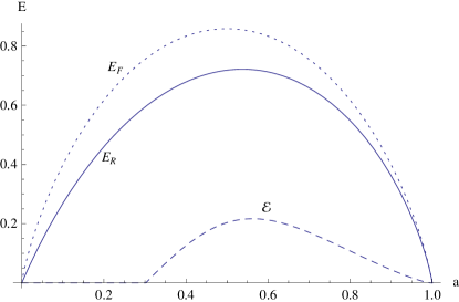
Figure 3: Entanglement of formation $E_{F}$ (dotted curve), relative entropy of entanglement $E_{R}$ (solid curve) and $\mathcal{E}=\max\left\{0,-\log_{2}\left(1-E_{G}\left(\rho\right)\right)-S\left(\rho\right)\right\}$ (dashed curve) of the state $\rho=p\ket{\psi}\bra{\psi}+\left(1-p\right)\ket{01}\bra{01}$ with $\ket{\psi}=\sqrt{a}\ket{01}+\sqrt{1-a}\ket{10}$ for $p=\frac{9}{10}$ as a function of $a$.

The inequality (30) becomes trivial for states with high entropy. As a nontrivial example we consider the two qubit state

$$\rho=p\ket{\psi}\bra{\psi}+\left(1-p\right)\ket{01}\bra{01},$$ (39)

with $\ket{\psi}=\sqrt{a}\ket{01}+\sqrt{1-a}\ket{10}$. This state was called generalised Vedral-Plenio state in Miranowicz2008 , where the authors showed that the closest separable state $\sigma$ with respect to the relative entropy of entanglement is given by

$$\sigma=\left(1-p+pa\right)\ket{01}\bra{01}+p\left(1-a\right)\ket{10}\bra{10}.$$ (40)

In Figure 2 and 3 we show the plot of $E_{F}$ (dotted curve), $E_{R}$ (solid curve) and $\mathcal{E}=\max\left\{0,-\log_{2}\left(1-E_{G}\left(\rho\right)\right)-S\left(\rho\right)\right\}$ (dashed curve) as a function of $a$ for $p=\frac{99}{100}$ and $p=\frac{9}{10}$ respectively. It can be seen that $\mathcal{E}$ drops quickly with increasing entropy of the state, and thus is nontrivial only for states close to pure states with high entanglement.

In Plenio2000 ; Plenio2001 the authors gave lower bounds for the relative entropy of entanglement in terms of the von Neumann entropies of the reduced states, which provide better lower bounds for $E_{R}$ than (30). Thus, the inequality (30) should be seen as a connection between the two entanglement measures $E_{R}$ and $E_{G}$, and not as an improved lower bound for $E_{R}$.

IV Entanglement measures for two qubits

IV.1 Bures measure of entanglement

We can use Proposition 1 to evaluate entanglement measures for two qubit states. From Vidal2000 ; Wei2003 we know the geometric measure for two-qubit states as a function of the concurrence, see eq. (14). Using this together with eq. (28) we find the fidelity of separability as function of the concurrence:

$$F_{s}(\rho)=\max_{\sigma\in S}F\left(\rho,\sigma\right)=\frac{1}{2}\left(1+\sqrt{1-C\left(\rho\right)^{2}}\right).$$ (41)

Now we are able to give an expression for the Bures measure of entanglement for two qubit states, remember its definition in eq. (3).

Proposition 3.

For any two qubit state $\rho$ the Bures measure of entanglement is given by

$$E_{B}\left(\rho\right)=2-2\sqrt{\frac{1+\sqrt{1-C\left(\rho\right)^{2}}}{2}}.$$ (42)

Note that for a maximally entangled state $E_{G}=\frac{1}{2}$ and $E_{B}=2-\sqrt{2}$. In order to compare these measures we renormalise them such that each of them becomes equal to $1$ for maximally entangled states. We show the result in Figure 4. There we also plot the Groverian measure of entanglement, see eq. (4).

Figure 4: Plot of the geometric measure of entanglement $E_{G}$, Bures measure of entanglement $E_{B}$ and Groverian measure of entanglement $E_{Gr}$ as a function of the concurrence $C$ for two qubit states. All measures were renormalised such that they reach $1$ for maximally entangled states.

IV.2 Measures induced by the geometric measure of entanglement

We consider now any generalised measure of entanglement for two qubit states $\rho$ which can be written as a function of the geometric measure of entanglement:

$$E_{f}\left(\rho\right)=f\left(E_{G}\left(\rho\right)\right).$$ (43)

Proposition 4.

Let $f\left(x\right)$ be any convex function that is nonnegative for $x\geq 0$ and obeys $f\left(0\right)=0$. Then for two qubits $E_{f}(\rho)=f\left(E_{G}\left(\rho\right)\right)$ is equal to its convex roof, that is

$$E_{f}\left(\rho\right)=\min\sum_{i}p_{i}E_{f}\left(\ket{\psi_{i}}\right)=f\left(\frac{1}{2}\left(1-\sqrt{1-C\left(\rho\right)^{2}}\right)\right),$$ (44)

where the minimisation is done over all pure state decompositions of $\rho$.

Proof.

From Wei2003 we know that the geometric measure of entanglement is a convex nonnegative function of the concurrence, see also (14) and Figure 4. As shown in Wei2003 , from convexity follows that $E_{G}$ and $E_{F}$ have identical optimal decompositions, and every state in this optimal decomposition has the same concurrence. This observation led directly to the expression (14) for $E_{G}$ of two qubit states.

As $f$ is convex, $E_{f}$ also is a convex function of the concurrence. To see this we note that convexity of $E_{G}$ implies

$$E_{G}\left(\sum_{i}p_{i}C_{i}\right)\leq\sum_{i}p_{i}E_{G}\left(C_{i}\right),$$ (45)

where we defined $E_{G}\left(C\right)=\frac{1}{2}(1-\sqrt{1-C^{2}})$. As $f\left(x\right)$ is convex, nonnegative and $f\left(0\right)=0$, it also must be monotonously increasing for $x\geq 0$. Thus we have

$$f\left(E_{G}\left(\sum_{i}p_{i}C_{i}\right)\right)\leq f\left(\sum_{i}p_{i}E_{G}\left(C_{i}\right)\right).$$ (46)

Now we can use convexity of $f$ to get

$$f\left(E_{G}\left(\sum_{i}p_{i}C_{i}\right)\right)\leq\sum_{i}p_{i}f\left(E_{G}\left(C_{i}\right)\right).$$ (47)

Defining $E_{f}\left(C\right)=f\left(E_{G}\left(C\right)\right)=f\left(\frac{1}{2}\left(1-\sqrt{1-C^{2}}\right)\right)$ the inequality above becomes

$$E_{f}\left(\sum_{i}p_{i}C_{i}\right)\leq\sum_{i}p_{i}E_{f}\left(C_{i}\right).$$ (48)

This proves that $E_{f}\left(C\right)$ is a convex function of the concurrence. Using the same argumentation as was used in Wei2003 to prove the expression (14) we see that (44) must hold. ∎

As an example consider the Bures measure of entanglement which can be written as $E_{B}\left(\rho\right)=E_{f}\left(\rho\right)$ with the convex function $f=2-2\sqrt{1-E_{G}\left(\rho\right)}$. Using Proposition 4 we see that for two qubits the Bures measure of entanglement is equal to its convex roof.

However, this might not be the case for a general higher-dimensional state $\rho$. To see this assume that $E_{B}\left(\rho\right)$ is equal to $\min\sum_{i}p_{i}E_{B}\left(\ket{\psi_{i}}\right)$. This means that $\sqrt{F_{s}\left(\rho\right)}$ is equal to $\max\sum_{i}p_{i}\sqrt{F_{s}\left(\ket{\psi_{i}}\right)}$. On the other hand, from Theorem 1 we know that

$$F_{s}\left(\rho\right)=\max\sum_{i}p_{i}F_{s}\left(\ket{\psi_{i}}\right),$$ (49)

and using monotonicity and concavity of the square root we see:

$$\sqrt{F_{s}\left(\rho\right)}=\max\sqrt{\sum_{i}p_{i}F_{s}\left(\ket{\psi_{i}}\right)}\geq\max\sum_{i}p_{i}\sqrt{F_{s}\left(\ket{\psi_{i}}\right)}.$$ (50)

The Bures measure of entanglement is equal to its convex roof if and only if the inequality (50) becomes an equality for all states $\rho$.

Finally we note, that any entanglement measure $E_{h}$ defined as $E_{h}\left(\rho\right)=\min_{\sigma\in S}h\left(F\left(\rho,\sigma\right)\right)$ with a monotonously decreasing nonnegative function $h$, $h\left(1\right)=0$, becomes $E_{h}\left(\rho\right)=h\left(F_{s}\left(\rho\right)\right)$, and can be evaluated exactly for two qubits using Proposition 1. An example of such a measure is the Bures measure of entanglement.

V Optimal decompositions w.r.t. geometric measure of entanglement and consequences for closest separable states

Let $\rho$ be an $n$-partite quantum state acting on a finite-dimensional Hilbert space $\mathcal{H}=\otimes_{i=1}^{n}\mathcal{H}_{i}$ of dimension $d$. A decomposition of a mixed state $\rho$ is a set $\left\{p_{i},\ket{\psi_{i}}\right\}$ with $p_{i}>0$, $\sum_{i}p_{i}=1$, and $\rho=\sum_{i}p_{i}\ket{\psi_{i}}\bra{\psi_{i}}$. Throughout this paper we will call a decomposition optimal if it minimises the geometric measure of entanglement, i.e. if $E_{G}\left(\rho\right)=\sum_{i}p_{i}E_{G}\left(\ket{\psi_{i}}\right)$. A separable state $\sigma$ is a closest separable state to $\rho$ if $E_{G}\left(\rho\right)=1-F\left(\rho,\sigma\right)$. In the following we will show how to find an optimal decomposition of $\rho$, given a closest separable state.

V.1 Equivalence between closest separable states and optimal decompositions

In the maximisation of $F\left(\rho,\sigma\right)$ we can restrict ourselves to separable states $\sigma$ acting on the same Hilbert space $\mathcal{H}$. To see this, note that this is obviously true for pure states, as we can always find a pure separable state $\ket{\phi}\in\mathcal{H}$ such that $\left|\braket{\psi}{\phi}\right|^{2}$ is maximal. (Extra dimensions cannot increase the overlap with the original state.) Let now $\sigma=\sum_{i}q_{i}\ket{\phi_{i}}\bra{\phi_{i}}$ be a closest separable state with purification $\ket{\phi}$ such that $F_{s}\left(\rho\right)=\left|\braket{\psi}{\phi}\right|^{2}$, where $\ket{\psi}$ is a purification of $\rho$. We can again write the purifications as

$$\ket{\psi} = \sum_{i}\sqrt{p_{i}}\ket{\psi_{i}}\ket{i},$$ (51)

$$\ket{\phi} = \sum_{j}\sqrt{q_{j}}\ket{\phi_{j}}\ket{j},$$ (52)

with separable pure states $\ket{\phi_{j}}$ such that $\sqrt{F_{s}\left(\ket{\psi_{i}}\right)}=\braket{\psi_{i}}{\phi_{i}}$. As the states $\ket{\phi_{j}}$ are elements of $\mathcal{H}$, the reduced state $\sigma=\mathrm{Tr}_{a}\left[\ket{\phi}\bra{\phi}\right]$ is a bounded operator acting on the same Hilbert space $\mathcal{H}$, $\mathrm{Tr}_{a}$ denotes partial trace over the ancillary Hilbert space spanned by the orthonormal basis $\left\{\ket{i}\right\}$.

Now we are in position to prove the following result.

Proposition 5.

Let $\rho$ be an $n$-partite quantum state acting on $\mathcal{H}=\otimes_{i=1}^{n}\mathcal{H}_{i}$. The separable state $\sigma=\sum_{j=1}^{s}q_{j}\ket{\phi_{j}}\bra{\phi_{j}}$ with $s\geq d$ separable pure states $\ket{\phi_{j}}$ and $\sum_{j=1}^{s}q_{j}=1$, $q_{i}\geq 0$, is the closest separable state if and only if there exists an optimal decomposition $\left\{p_{i},\ket{\psi_{i}}\right\}_{i=1}^{s}$ with $s\geq d$ elements such that holds: $\sqrt{F_{s}\left(\ket{\psi_{i}}\right)}=\braket{\psi_{i}}{\phi_{i}}$ and $q_{i}=\frac{p_{i}F_{s}\left(\ket{\psi_{i}}\right)}{\sum_{k}p_{k}F_{s}\left(\ket{\psi_{k}}\right)}$.

Proof.

In the following $\left\{\ket{i}\right\}$ denotes a basis on the ancillary Hilbert space $\mathcal{H}_{a}$. The closest separable state $\sigma=\sum_{j=1}^{s}q_{j}\ket{\phi_{j}}\bra{\phi_{j}}$ can be purified by

$$\ket{\phi}=\sum_{j=1}^{s}\sqrt{q_{j}}\ket{\phi_{j}}\ket{j}.$$ (53)

We write a purification of the state $\rho$ as

$$\ket{\psi}=\sum_{i=1}^{s}\sqrt{\lambda_{i}}\ket{\lambda_{i}}U\ket{i},$$ (54)

where $\lambda_{i}$ are the eigenvalues and $\ket{\lambda_{i}}$ are the corresponding eigenstates of $\rho$, with $\lambda_{i}=0$ for $i\geq d$, and $U$ is a unitary acting on the ancillary Hilbert space $\mathcal{H}_{a}$. According to Uhlmann’s theorem Uhlmann1976 ; Nielsen2000 it holds:

$$\left|\braket{\psi}{\phi}\right|^{2}\leq F\left(\rho,\sigma\right)=F_{s}\left(\rho\right).$$ (55)

In the following let $U$ be a unitary such that equality is achieved in (55); its existence is assured by Uhlmann’s theorem. Writing $U=\sum_{k,l=1}^{s}u_{kl}\ket{k}\bra{l}$ in (54) we get:

$$\ket{\psi} = \sum_{k,l=1}^{s}u_{kl}\sqrt{\lambda_{l}}\ket{\lambda_{l}}\ket{k}=\sum_{k=1}^{s}\sqrt{p_{k}}\ket{\psi_{k}}\ket{k}$$ (56)

with $\sqrt{p_{k}}\ket{\psi_{k}}=\sum_{l=1}^{s}u_{kl}\sqrt{\lambda_{l}}\ket{\lambda_{l}}$. Note that $\left\{p_{k},\ket{\psi_{k}}\right\}_{k=1}^{s}$ is a decomposition of $\rho$.

We will now show that $\left\{p_{k},\ket{\psi_{k}}\right\}_{k=1}^{s}$ is an optimal decomposition by showing that $\left|\braket{\psi}{\phi}\right|^{2}=\sum_{i}p_{i}F_{s}\left(\ket{\psi_{i}}\right)$. As we chose the purifications such that $\left|\braket{\psi}{\phi}\right|^{2}=F_{s}\left(\rho\right)$, this will complete the proof. Computing the overlap $\left|\braket{\psi}{\phi}\right|^{2}$ using (53) and (56) we get:

$$\left|\braket{\psi}{\phi}\right|^{2}=\left|\sum_{i}\sqrt{p_{i}q_{i}}\braket{\psi_{i}}{\phi_{i}}\right|^{2}.$$ (57)

As in the proof of Theorem 1, maximality of (57) implies that $\left|\braket{\psi_{i}}{\phi_{i}}\right|=\sqrt{F_{s}\left(\ket{\psi_{i}}\right)}$ and $q_{i}=\frac{p_{i}F_{s}\left(\ket{\psi_{i}}\right)}{\sum_{k}p_{k}F_{s}\left(\ket{\psi_{k}}\right)}$. Then we immediately see that $\left\{p_{k},\ket{\psi_{k}}\right\}_{k=1}^{s}$ is optimal, because $F_{s}\left(\rho\right)=\left|\braket{\psi}{\phi}\right|^{2}=\sum_{i=1}^{s}p_{i}F_{s}\left(\ket{\psi_{i}}\right)$, which is exactly the optimality condition.

So far we proved the existence of an optimal decomposition $\left\{p_{i},\ket{\psi_{i}}\right\}$ with the property $\sqrt{F_{s}\left(\ket{\psi_{i}}\right)}=\braket{\psi_{i}}{\phi_{i}}$ starting from the existence of the closest separable state $\sigma=\sum_{j=1}^{s}q_{j}\ket{\phi_{j}}\bra{\phi_{j}}$. Now we will prove the inverse direction. Given an optimal decomposition $\left\{p_{i},\ket{\psi_{i}}\right\}_{i=1}^{s}$ we will find a closest separable state. We again define the purifications of $\rho$ and $\sigma$ as

$$\ket{\psi} = \sum_{i=1}^{s}\sqrt{p_{i}}\ket{\psi_{i}}\otimes\ket{i},$$ (58)

$$\ket{\phi} = \sum_{j=1}^{s}\sqrt{q_{j}}\ket{\phi_{j}}\otimes\ket{j},$$ (59)

where we define the states $\ket{\phi_{j}}$ to be separable and to have maximal overlap with $\ket{\psi_{j}}$, i.e. $\braket{\psi_{j}}{\phi_{j}}=\sqrt{F_{s}\left(\ket{\psi_{j}}\right)}$. The real numbers $q_{j}$ are defined as follows: $q_{j}=\frac{p_{j}F_{s}\left(\ket{\psi_{j}}\right)}{\sum_{k}p_{k}F_{s}\left(\ket{\psi_{k}}\right)}$. Now we note that $\left|\braket{\psi}{\phi}\right|^{2}=F_{s}\left(\rho\right)$ because the decomposition $\left\{p_{i},\ket{\psi_{i}}\right\}$ was defined to be optimal. Thus we see that there exists no purification $\ket{\phi^{\prime}}$ such that $\left|\braket{\psi}{\phi^{\prime}}\right|>\left|\braket{\psi}{\phi}\right|$. Together with Uhlmann’s theorem this implies that $F\left(\rho,\sigma\right)=F_{s}\left(\rho\right)$.

∎

V.2 Caratheodory bound

Now we are in position to show that the number of elements in an optimal decomposition (w.r.t. the geometric measure of entanglement) is bounded from above by the Caratheodory bound.

Corollary 1.

For any state $\rho$ acting on a Hilbert space of dimension $d$ always exists an optimal (w.r.t. the geometric measure of entanglement) decomposition $\left\{p_{i},\ket{\psi_{i}}\right\}_{i=1}^{s}$ such that $s\leq d^{2}$.

Proof.

Let $\sigma$ be a closest separable state. From Caratheodory’s theorem Horodecki1997 ; Vedral1998 follows that $\sigma$ can be written as a convex combination of $s\leq d^{2}$ pure separable states. According to Proposition 5 the state $\sigma$ can be used to find an optimal decomposition with $s$ elements. ∎

VI Structure of optimal decomposition w.r.t. geometric measure of entanglement

In this section we will show that the optimal decomposition of $\rho$ with respect to the geometric measure of entanglement has a certain symmetric structure.

VI.1 $n$-partite states

First we derive the structure of an optimal decomposition $\left\{p_{i},\ket{\psi_{i}}\right\}$ for a general $n$-partite state.

Proposition 6.

Every optimal decomposition $\left\{p_{i},\ket{\psi_{i}}\right\}_{i=1}^{s}$ must have the following structure:

$$\sqrt{F_{s}\left(\ket{\psi_{k}}\right)}\braket{\psi_{i}}{\phi_{k}}=\sqrt{F_{s}\left(\ket{\psi_{i}}\right)}\braket{\phi_{i}}{\psi_{k}}$$ (60)

for all $1\leq i,k\leq s$. Here the states $\ket{\phi_{i}}$ are separable and have the property $\braket{\phi_{i}}{\psi_{i}}=\sqrt{F_{s}\left(\ket{\psi_{i}}\right)}$.

Eq. (60) represent a nonlinear system of equations. Finding all solutions of it is equivalent to computing the optimal decomposition of $\rho$. For pure states our result reduces to the nonlinear eigenproblem given in equations (5a) and (5b) in Wei2003 .

Proof.

Let the states $\ket{i}$ denote an orthonormal basis on the ancillary Hilbert space $\mathcal{H}_{a}$. Let $\ket{\psi}=\sum_{i}\sqrt{p_{i}}\ket{\psi_{i}}\ket{i}$ and $\ket{\phi}=\sum_{j}\sqrt{q_{j}}\ket{\phi_{j}}\ket{j}$ be purifications of $\rho$ and $\sigma$, respectively, such that $\left\{p_{i},\ket{\psi_{i}}\right\}$ is an optimal decomposition of $\rho$, $\braket{\psi_{i}}{\phi_{i}}=\sqrt{F_{s}\left(\ket{\psi_{i}}\right)}$ and $q_{i}=\frac{p_{i}F_{s}\left(\ket{\psi_{i}}\right)}{\sum_{k}p_{k}F_{s}\left(\ket{\psi_{k}}\right)}$. This implies that

$$F_{s}\left(\rho\right)=\left|\braket{\psi}{\phi}\right|^{2}=\sum_{i}\left|\bra{\psi}\left(\ket{\phi_{i}}\otimes\ket{i}\right)\right|^{2}.$$ (61)

Optimality implies that $\left|\braket{\psi}{\phi}\right|^{2}$ is stationary under unitaries acting on the ancillary Hilbert space $\mathcal{H}_{a}$ (for stationarity under unitaries acting on the original space see subsection VI.5), that is

$$\frac{d}{dt}\left|\braket{\psi}{e^{itH_{a}}}{\phi}\right|_{t=0}^{2}=0$$ (62)

for any Hermitian $H_{a}=H_{a}^{\dagger}$ acting on $\mathcal{H}_{a}$ and the derivative is taken at $t=0$. Using (61) we can write

$$\left|\braket{\psi}{e^{itH_{a}}}{\phi}\right|^{2} = \sum_{k}\left|\bra{\psi}\left(\ket{\phi_{k}}e^{itH_{a}}\ket{k}\right)\right|^{2}.$$ (63)

The derivative at $t=0$ becomes:

$$\frac{d}{dt}\left|\braket{\psi}{e^{itH_{a}}}{\phi}\right|_{t=0}^{2}=\mathrm{Tr}_{a}\left[H_{a}\cdot\mathrm{Tr}_{\bar{a}}\left[\sum_{k}\left(A_{k}+A_{k}^{\dagger}\right)\right]\right]$$ (64)

with $A_{k}=i\left(\ket{\phi_{k}}\bra{\phi_{k}}\otimes\ket{k}\bra{k}\right)\ket{\psi}\bra{\psi}$ and $\mathrm{Tr}_{\bar{a}}$ means partial trace over all parts except for the ancillary space $\mathcal{H}_{a}$. Using $\left(\bra{\phi_{k}}\bra{k}\right)\ket{\psi}=\sqrt{p_{k}}\sqrt{F_{s}\left(\ket{\psi_{k}}\right)}$ we can write $A_{k}$ as

$$A_{k}=i\sqrt{p_{k}F_{s}\left(\ket{\psi_{k}}\right)}\ket{\phi_{k}}\ket{k}\bra{\psi}.$$ (65)

Expression (64) has to be zero for all Hermitian $H_{a}$ which can only be true if $\mathrm{Tr}_{\bar{a}}\left[\sum_{k}\left(A_{k}+A_{k}^{\dagger}\right)\right]=0$ which is equivalent to

$$\sum_{k}\mathrm{Tr}_{\bar{a}}\left[\sqrt{p_{k}F_{s}\left(\ket{\psi_{k}}\right)}\ket{\phi_{k}}\ket{k}\bra{\psi}\right]$$ (66)

$$=\sum_{k}\mathrm{Tr}_{\bar{a}}\left[\sqrt{p_{k}F_{s}\left(\ket{\psi_{k}}\right)}\ket{\psi}\bra{k}\bra{\phi_{k}}\right].$$

With $\ket{\psi}=\sum_{i}\sqrt{p_{i}}\ket{\psi_{i}}\ket{i}$ we get

$$\sum_{i,k}\sqrt{p_{k}p_{i}F_{s}\left(\ket{\psi_{k}}\right)}\braket{\psi_{i}}{\phi_{k}}\ket{k}\bra{i}$$ (67)

$$=\sum_{i,k}\sqrt{p_{i}p_{k}F_{s}\left(\ket{\psi_{k}}\right)}\braket{\phi_{k}}{\psi_{i}}\ket{i}\bra{k}.$$

Using orthogonality of $\left\{\ket{i}\right\}$ completes the proof. ∎

VI.2 Bipartite states

Let us illustrate the structure of an optimal decomposition with the example of bipartite states. We consider the expression (60) for a bipartite mixed state $\rho$ with optimal decomposition $\left\{p_{i},\ket{\psi_{i}}\right\}$. In this case it is possible to write the Schmidt decomposition of the pure states $\ket{\psi_{i}}$ as follows:

$$\ket{\psi_{i}}=\sum_{j}\lambda_{i,j}\ket{j_{i}^{\left(1\right)}}\ket{j_{i}^{\left(2\right)}}$$ (68)

with $\sum_{j}\lambda_{i,j}^{2}=1$, and the Schmidt coefficients are in decreasing order, i.e. $\lambda_{i,1}\geq\lambda_{i,2}\geq...>0$. The separable states $\ket{\phi_{i}}$ that have the highest overlap with $\ket{\psi_{i}}$ are given by

$$\ket{\phi_{i}}=\ket{1_{i}^{\left(1\right)}}\ket{1_{i}^{\left(2\right)}},$$

and $\sqrt{F_{s}\left(\ket{\psi_{i}}\right)}=\lambda_{i,1}$. With this in mind expression (60) reduces to

$$\lambda_{k,1}\braket{\psi_{i}}{1_{k}^{\left(1\right)}}\ket{1_{k}^{\left(2\right)}}=\lambda_{i,1}\bra{1_{i}^{\left(1\right)}}\braket{1_{i}^{\left(2\right)}}{\psi_{k}}$$ (69)

for all $i$, $k$.

VI.3 Qubit-qudit states

Let now the first system be a qubit, that is $d_{1}=2$. In this case we can set $\lambda_{k,1}=\cos\alpha_{k}$ and $\lambda_{k,2}=\sin\alpha_{k}$, with $\cos\alpha_{k}\geq\sin\alpha_{k}$. With $\ket{\psi_{k}}=\cos\alpha_{k}\ket{11}+\sin\alpha_{k}\ket{22}$ we get from eq. (69)

$$\cos\alpha_{k}\sin\alpha_{i}\left(\braket{2_{i}^{\left(1\right)}}{1_{k}^{\left(1\right)}}\braket{2_{i}^{\left(2\right)}}{1_{k}^{\left(2\right)}}\right)$$ (70)

$$=\cos\alpha_{i}\sin\alpha_{k}\left(\braket{1_{i}^{\left(1\right)}}{2_{k}^{\left(1\right)}}\braket{1_{i}^{\left(2\right)}}{2_{k}^{\left(2\right)}}\right).$$

Noting that $\left|\braket{2_{i}^{\left(1\right)}}{1_{k}^{\left(1\right)}}\right|=\left|\braket{1_{i}^{\left(1\right)}}{2_{k}^{\left(1\right)}}\right|$ it follows that

$$\frac{\tan\alpha_{i}}{\tan\alpha_{k}}=\left|\frac{\braket{1_{i}^{\left(2\right)}}{2_{k}^{\left(2\right)}}}{\braket{2_{i}^{\left(2\right)}}{1_{k}^{\left(2\right)}}}\right|.$$ (71)

It is interesting to mention that in the case $d_{2}=2$ we can simplify (71) to $\tan\alpha_{i}=\tan\alpha_{k}$. This means that in the optimal decomposition $\left\{p_{i},\ket{\psi_{i}}\right\}$ of a two-qubit state all states $\ket{\psi_{i}}$ have the same Schmidt coefficients, a result already known from Wootters1998 .

VI.4 Nonoptimal stationary decompositions

Note that expression (60) is necessary, but not sufficient for a decomposition to be optimal. To prove this we will give two non-optimal decompositions that satisfy (60).

VI.4.1 Bell diagonal states

Consider the state

$$\rho=\frac{1}{2}\ket{\psi^{+}}\bra{\psi^{+}}+\frac{1}{2}\ket{\phi^{+}}\bra{\phi^{+}},$$ (72)

with $\ket{\psi^{+}}=\frac{1}{\sqrt{2}}\left(\ket{01}+\ket{10}\right)$ and $\ket{\phi^{+}}=\frac{1}{\sqrt{2}}\left(\ket{00}+\ket{11}\right)$. It is well known that the state (72) is separable, and thus the decomposition into Bell states cannot be optimal. On the other hand, it is easy to see that this decomposition satisfies (60).

VI.4.2 Separable states

Now we will give a more complicated example. We call a decomposition $\left\{p_{i},\ket{\psi_{i}}\right\}_{i=1}^{s}$ $s$-optimal if for a given number of terms $s$ there is no decomposition $\left\{q_{i},\ket{\phi_{i}}\right\}_{i=1}^{s}$ such that $\sum_{i=1}^{s}q_{i}E_{G}\left(\ket{\phi_{i}}\right)<\sum_{i=1}^{s}p_{i}E_{G}\ket{\psi_{i}}$. It is known Horodecki2009 that there exist separable states $\rho$ of dimension $d$ with the property that any $d$-optimal decomposition is not separable and thus not optimal. Let $\left\{p_{i},\ket{\psi_{i}}\right\}_{i=1}^{d}$ be a $d$-optimal decomposition of such a state $\rho$.

We write a purification of $\rho$ as $\ket{\psi}=\sum_{i=1}^{d}\sqrt{p_{i}}\ket{\psi_{i}}\ket{i}$. Further we define separable states $\ket{\phi_{i}}$ such that $\braket{\psi_{i}}{\phi_{i}}=\sqrt{F_{s}\left(\ket{\psi_{i}}\right)}$, $q_{i}=\frac{p_{i}F_{s}\left(\ket{\psi_{i}}\right)}{\sum_{k}p_{k}F_{s}\left(\ket{\psi_{k}}\right)}$ and $\ket{\phi}=\sum_{j=1}^{d}\sqrt{q_{j}}\ket{\phi_{j}}\ket{j}$. Then it holds that:

$$\left|\braket{\psi}{\phi}\right|^{2}=\sum_{i=1}^{d}p_{i}F_{s}\left(\ket{\psi_{i}}\right)^{2}.$$ (73)

From $d$-optimality of $\left|\braket{\psi}{\phi}\right|^{2}$ follows that for all Hermitian matrices acting on a $d$-dimensional Hilbert space $\mathcal{H}_{a}$

$$\frac{d}{dt}\left|\braket{\psi}{e^{itH_{a}}}{\phi}\right|_{t=0}^{2}=0$$ (74)

holds. We will now show that $\frac{d}{dt}\left|\braket{\psi}{e^{itH_{a}}}{\phi}\right|_{t=0}^{2}=0$ also holds for dim$\left(\mathcal{H}_{a}\right)\geq d$. This means that adding more dimensions to the ancillary Hilbert space will not help. Doing the same calculation as in the proof of Proposition 6 we get:

$$\frac{d}{dt}\left|\braket{\psi}{e^{itH_{a}}}{\phi}\right|_{t=0}^{2}=\mathrm{Tr}_{a}\left[H_{a}\cdot\mathrm{Tr}_{\bar{a}}\left[\sum_{k=1}^{d\left(\mathcal{H}_{a}\right)}\left(A_{k}+A_{k}^{\dagger}\right)\right]\right]$$ (75)

with $A_{k}=i\sqrt{p_{k}F_{s}\left(\ket{\psi_{k}}\right)}\ket{\phi_{k}}\ket{k}\bra{\psi}$. Note that $A_{k}$ is nonzero only for $k\leq d$, because $p_{k}=0$ otherwise. Thus we can restrict ourselves to $k\leq d$ in the calculation, which is equivalent to setting dim$\left(\mathcal{H}_{a}\right)=d$. Then (74) implies $\mathrm{Tr}_{\bar{a}}\left[\sum_{k=1}^{d\left(\mathcal{H}_{a}\right)}\left(A_{k}+A_{k}^{\dagger}\right)\right]=0$ and it follows that (74) holds for arbitrary $d\left(\mathcal{H}_{a}\right)\geq d$.

VI.5 Stationarity on the original subspace

In Proposition 6 we used the argument that in the optimal case $\left|\braket{\psi}{\phi}\right|^{2}$ has to be stationary under unitaries acting on the ancillary Hilbert space $\mathcal{H}_{a}$. In (61) we could rewrite this expression as

$$F_{s}\left(\rho\right)=\left|\braket{\psi}{\phi}\right|^{2}=\sum_{i}\left|\braket{\psi}{\phi_{i}}\ket{i}\right|^{2},$$

where all $\ket{\phi_{i}}$ are separable. We can also demand $\sum_{i}\left|\braket{\psi}{\phi_{i}}\ket{i}\right|^{2}$ to be stationary under (separable) unitaries acting on the original Hilbert space of the states $\ket{\phi_{i}}$. From this procedure we will gain stationary equations describing the states $\ket{\phi_{i}}$. However, we already know that in the optimal case we can choose $\ket{\phi_{i}}$ to be the closest separable state to $\ket{\psi_{i}}$, that is $\braket{\psi_{i}}{\phi_{i}}=\sqrt{F_{s}\left(\ket{\psi_{i}}\right)}$, such that this method does not give new results.

VII Concluding remarks

We have shown in this paper that the geometric measure of entanglement belongs to two classes of entanglement measures. Namely it is a convex roof measure and also a distance measure of entanglement. As an application we gave a closed formula for the Bures measure of entanglement for two qubits. We also note that the revised geometric measure of entanglement defined in Cao2007 is equal to the original geometric measure of entanglement.

We furthermore proved that the problems of finding a closest separable state and finding an optimal decomposition are equivalent. We used this insight to bound the number of elements in an optimal decomposition (with respect to the geometric measure of entanglement). It turns out that the bound is exactly given by the Caratheodory bound.

Finally, we obtained stationary equations which ensure optimality of a decomposition. For the case of two qubits these equations lead to the known fact that each constituting state of an optimal decomposition has equal concurrence. Our equations hold for any dimension. However, they are only necessary, not sufficient for a decomposition to be optimal. Given an arbitrary decomposition, they provide a simple test whether the decomposition may be optimal.

Appendix A Geometric measure of a convex set

In Theorem 1 we stated that if $S$ is the set of separable states it holds:

$$F_{s}\left(\rho\right)=\max\sum_{i}p_{i}F_{s}\left(\ket{\psi_{i}}\right),$$ (76)

where $F_{s}$ is the maximal fidelity between $\rho$ and the set of separable states: $F_{s}\left(\rho\right)=\max_{\sigma\in S}F\left(\rho,\sigma\right)$ and the maximisation is done over all pure state decompositions of $\rho$. In the following we will generalise this result to arbitrary convex sets.

Let $X$ be a set of states $\left\{\sigma_{k}\right\}$ and $C$ be a set containing all convex combinations of the elements of $X$, these are states $\sigma$ such that holds:

$$\sigma=\sum_{k}q_{k}\sigma_{k}$$ (77)

with $q_{k}\geq 0$, $\sum_{k}q_{k}=1$. We define the quantities $F_{X}\left(\rho\right)$ and $F_{C}\left(\rho\right)$ to be the maximal fidelity between $\rho$ and an element of $X$ and $C$ respectively:

$$F_{X}\left(\rho\right) = \max_{\sigma\in X}F\left(\rho,\sigma\right),$$ (78)

$$F_{C}\left(\rho\right) = \max_{\sigma\in C}F\left(\rho,\sigma\right).$$ (79)

Theorem 2.

For an arbitrary quantum state $\rho$ and a convex set of states $C$ holds

$$F_{C}\left(\rho\right) = \max_{\rho=\sum_{k}p_{k}\rho_{k}}\sum_{i}p_{i}F_{X}\left(\rho_{i}\right),$$ (80)

where the maximisation is done over all decompositions of $\rho=\sum_{i}p_{i}\rho_{i}$, $p_{i}\geq 0$.

Proof.

The proof is a modification of the proof of Theorem 1. According to Uhlmann’s theorem (Nielsen2000, , page 411) holds:

$$F\left(\rho,\sigma\right)=\max_{\ket{\phi}}\left|\braket{\psi}{\phi}\right|^{2},$$ (81)

$\ket{\psi}$ is a purification of $\rho$ and the maximisation is done over all purifications of $\sigma$ denoted by $\ket{\phi}$.

In order to find $F_{C}\left(\rho\right)$ we have to maximise $\left|\braket{\psi}{\phi}\right|^{2}$ over purifications $\ket{\phi}$ of all states of the form $\sigma=\sum_{k}q_{k}\sigma_{k}$, $\sigma_{k}\in X$. Using similar arguments as in the proof of the Theorem 1 we see that the purifications can always be written as

$$\ket{\psi} = \sum_{i}\sqrt{p_{i}}\left(\sum_{j}\sqrt{p_{i,j}}\ket{\psi_{i,j}}\otimes\ket{i,j}\right),$$ (82)

$$\ket{\phi} = \sum_{k}\sqrt{q_{k}}\left(\sum_{l}\sqrt{q_{k,l}}\ket{\phi_{k,l}}\otimes\ket{k,l}\right),$$ (83)

with $\braket{i,j}{k,l}=\delta_{ik}\delta_{jl}$. In the maximisation of $\left|\braket{\psi}{\phi}\right|^{2}$ we are free to choose the states $\ket{\phi_{k,l}}$ under the restriction that $\sum_{l}\sqrt{q_{k,l}}\ket{\phi_{k,l}}\otimes\ket{k,l}$ purifies $\sigma_{k}\in X$, the probabilities $q_{k}>0$ are restricted only by $\sum_{k}q_{k}=1$. We are also free to choose $\left\{\ket{\psi_{i,j}}\right\}$, $\left\{p_{i}\right\}$ and $\left\{p_{i,j}\right\}$ under the restriction $\rho=\sum_{i,j}p_{i}p_{ij}\ket{\psi_{i,j}}\bra{\psi_{i,j}}$. With this in mind we get:

$$\left|\braket{\psi}{\phi}\right|=\left|\sum_{i,k}\sqrt{p_{i}q_{k}}a_{i,k}\right|,$$ (84)

with $a_{i,k}$ being the product of the purifications of $\rho_{i}$ and $\sigma_{k}$:

$$a_{i,k}=\left(\sum_{j}\sqrt{p_{i,j}}\bra{\psi_{i,j}}\otimes\bra{i,j}\right)\left(\sum_{l}\sqrt{q_{k,l}}\ket{\phi_{k,l}}\otimes\ket{k,l}\right).$$

Now we optimise over $\left\{q_{k,l},\ket{\phi_{k,l}}\right\}$ with the result

$$a_{i,k}=\sqrt{F_{X}\left(\rho_{i}\right)}\delta_{ik}$$ (85)

and thus

$$\max_{\left\{q_{k,l},\ket{\phi_{k,l}}\right\}}\left|\braket{\psi}{\phi}\right|=\sum_{i}\sqrt{q_{i}p_{i}}\sqrt{F_{X}\left(\rho_{i}\right)}.$$ (86)

Now we do the optimisation over $q_{i}$. Using Lagrange multipliers we get

$$\sqrt{q_{i}}=\frac{\sqrt{p_{i}}\sqrt{F_{X}\left(\rho_{i}\right)}}{\sqrt{\sum_{k}p_{k}F_{X}\left(\rho_{k}\right)}},$$ (87)

with the result

$$\max_{\left\{q_{j},q_{k,l},\ket{\phi_{k,l}}\right\}}\left|\braket{\psi}{\phi}\right|^{2}=\sum_{i}p_{i}F_{X}\left(\rho_{i}\right).$$ (88)

In the last step we do the maximisation over all decompositions $\left\{p_{i},\rho_{i}\right\}$ of the given state $\rho$ which leads to the final result

$$F_{C}\left(\rho\right)=\max\left|\braket{\psi}{\phi}\right|^{2}=\max\sum_{i}p_{i}F_{X}\left(\rho_{i}\right).$$ (89)

∎

References

- (1) A. Einstein, B. Podolsky, and N. Rosen, Phys. Rev. 47, 777 (1935)
- (2) R. Horodecki, P. Horodecki, M. Horodecki, and K. Horodecki, Rev. Mod. Phys. 81, 865 (2009), arXiv:quant-ph/0702225v2
- (3) M. B. Plenio and S. Virmani, Quant. Inf. Comp. 7, 1 (2007), arXiv:quant-ph/0504163v3
- (4) R. F. Werner, Phys. Rev. A 40, 4277 (1989)
- (5) Note that the distillable entanglement does not satisfy this criterion, i.e. it can be zero on entangled states. However it is also accepted as a measure of entanglement Horodecki2009 .
- (6) V. Vedral, M. B. Plenio, M. A. Rippin, and P. L. Knight, Phys. Rev. Lett. 78, 2275 (1997), arXiv:quant-ph/9702027v1
- (7) V. Vedral and M. B. Plenio, Phys. Rev. A 57, 1619 (1998), arXiv:quant-ph/9707035v2
- (8) A. Uhlmann, Rep. Math. Phys. 9, 273 (1976)
- (9) O. Biham, M. A. Nielsen, and T. J. Osborne, Phys. Rev. A 65, 062312 (2002), arXiv:quant-ph/0112097v1
- (10) D. Shapira, Y. Shimoni, and O. Biham, Phys. Rev. A 73, 044301 (2006), arXiv:quant-ph/0508108v1
- (11) A. Uhlmann, Open Sys. Inf. Dyn. 5, 209 (1997), arXiv:quant-ph/9704017v2
- (12) T.-C. Wei and P. M. Goldbart, Phys. Rev. A 68, 042307 (2003), arXiv:quant-ph/0307219v1
- (13) A. Shimony, Annals of the New York Academy of Sciences 755, 675 (1995)
- (14) H. Barnum and N. Linden, J. Phys. A: Math. Gen. 34, 6787 (2001), arXiv:quant-ph/0103155v1
- (15) C. H. Bennett, D. P. DiVincenzo, J. A. Smolin, and W. K. Wootters, Phys. Rev. A 54, 3824 (1996), arXiv:quant-ph/9604024v2
- (16) W. K. Wootters, Phys. Rev. Lett. 80, 2245 (1998), arXiv:quant-ph/9709029v2
- (17) G. Vidal, Phys. Rev. A 62, 062315 (2000), arXiv:quant-ph/0003002v1
- (18) D. Gross, S. T. Flammia, and J. Eisert, Phys. Rev. Lett. 102, 190501 (2009), arXiv:0810.4331 [quant-ph]
- (19) O. Gühne, M. Reimpell, and R. F. Werner, Phys. Rev. Lett. 98, 110502 (2007), arXiv:quant-ph/0607163v2
- (20) O. Gühne, G. Tóth, P. Hyllus, and H. J. Briegel, Phys. Rev. Lett. 95, 120405 (2005), arXiv:quant-ph/0410059
- (21) M. A. Nielsen and I. L. Chuang, Quantum Computation and Quantum Information (Cambridge University Press, 2000) ISBN 521635039
- (22) L. P. Hughston, R. Jozsa, and W. K. Wootters, Phys. Lett. A 183, 14 (1993)
- (23) T.-C. Wei, M. Ericsson, P. M. Goldbart, and W. J. Munro, Quantum Inform. Compu. 4, 252 (2004), arXiv:quant-ph/0405002v2
- (24) A. Miranowicz and S. Ishizaka, Phys. Rev. A 78, 032310 (2008), arXiv:0805.3134v3
- (25) M. B. Plenio, S. Virmani, and P. Papadopoulos, J. Phys. A: Math. Gen. 33, L193 (2000), arXiv:quant-ph/0002075v2
- (26) M. B. Plenio and V. Vedral, J. Phys. A: Math. Gen. 34, 6997 (2001), arXiv:quant-ph/0010080v1
- (27) P. Horodecki, Phys. Lett. A 232, 333 (1997), arXiv:quant-ph/9703004v2
- (28) Y. Cao and A. M. Wang, J. Phys. A: Math. Theor. 40, 3507 (2007), arXiv:quant-ph/0701099v2