Multiple stellar populations and their influence on blue stragglers

Abstract

It has become clear in recent years that globular clusters are not simple stellar populations, but may host chemically distinct sub-populations, typically with an enhanced helium abundance. These helium-rich populations can make up a substantial fraction of all cluster stars.

One of the proposed formation channels for blue straggler stars is the physical collision and merger of two stars. In the context of multiple populations, collisions between stars with different helium abundances should occur and contribute to the observed blue straggler population. This will affect the predicted blue straggler colour and luminosity function.

We quantify this effect by calculating models of mergers resulting from collisions between stars with different helium abundances and using these models to model a merger population. We then compare these results to four observed clusters, NGC 1851, NGC 2808, NGC 5634 and NGC 6093.

As in previous studies our models deviate from the observations, particularly in the colour distributions. However, our results are consistent with observations of multiple populations in these clusters. In NGC 2808, our best fitting models include normal and helium enhanced populations, in agreement with helium enhancement inferred in this cluster. The other three clusters show better agreement with models that do not include helium enhancement. We discuss future prospects to improve the modelling of blue straggler populations and the role that the models we present here can play in such a study.

1 Introduction

Blue stragglers are stars that appear on the extension of the main sequence in both open and globular clusters and have been studied extensively since their original discovery by Sandage (1953). Their existence cannot be explained by conventional stellar evolution models. Two formation channels have been discussed extensively in the literature, one using stellar collisions (Lombardi et al., 1995; Sills et al., 1997; Sills et al., 2005; Glebbeek & Pols, 2008) and one using binary evolution (Chen & Han, 2004, 2008, 2009). So far observations do not clearly indicate which of these formation mechanisms is the dominant one, or even if there is a dominant formation mechanism (Knigge et al., 2009). Neither formation mechanism has been able to completely account for the properties of the observed blue straggler populations, in particular the colour and magnitude distributions.

Star to star abundance variations in globular clusters, originally known as “globular cluster abundance anomalies”, have been known for a long time (see Gratton et al. 2004 for a recent review). The observed abundance patterns indicate that at least some of the globular cluster stars (up to 50% of the present day population) contain material that has undergone partial hydrogen burning at high temperatures. The most famous example is the so-called oxygen-sodium anti-correlation. To date, abundance variations have been observed in all clusters where the observational data has sufficient resolution to detect them. Despite work by several groups, the origin of these abundance variations is still unclear. The leading models propose that material has been processed by AGB stars (Ventura et al., 2001, 2002; Ventura & D’Antona, 2005) or rapidly rotating massive stars (Decressin et al., 2007) before being returned to the interstellar medium to form new stars. An alternative scenario involves non-conservative mass transfer in a binary system (de Mink et al., 2009). Since the main product of hydrogen burning is helium, this polluted material is also expected to be relatively helium rich and we may therefore expect to find a helium enhanced sub-population among cluster stars.

The first evidence for the existence of multiple populations in gobular clusters comes from the discovery of a split giant branch in $\omega$ Cen (Pancino et al., 2000). It was later shown that the sub giant branch (Ferraro et al., 2004) and the main sequence (Bedin et al., 2004) are likewise split in multiple sequences, which is interpreted as a spread in helium abundance (Piotto et al., 2005). D’Antona et al. (2005) predicted the existence of multiple populations in NGC 2808 based on the observed width of the main sequence band. Detailed observations by Piotto et al. (2007) found that the main sequence of NGC 2808 indeed splits into three distinct sequences. Milone et al. (2008) reported the existence of a double sub-giant branch in NGC 1851.

If collisions contribute to blue straggler formation and the different sub-populations have a comparable number of stars, then collisions between stars from a helium-rich and a helium-normal population must contribute to the observed blue straggler population. A blue straggler that is formed from a collision between a helium normal and a helium-rich star will have a higher helium abundance in its interior than a blue straggler formed by a collision between equivalent stars with the same helium abundance. This has the effect of making the star brighter, even if the material is not mixed efficiently (Glebbeek et al., 2008). Therefore, collisions involving stars from different populations should be taken into consideration when constructing the blue straggler colour and luminosity functions in clusters with multiple populations.

Here we explore the results of such a calculation.

2 Computational set-up

We use the STARS code (§2.2) to calculate the evolution tracks of both the progenitor stars and the collision products. The structure of the collision products themselves is calculated using the MMAS code (§2.1).

The parameter space for our models consists of the masses of the two colliding stars, $M_{1}$ and $M_{2}$, the time of collision $t_{\mathrm{coll}}$ and the helium abundance of the colliding stars, $Y_{1}$ and $Y_{2}$. In principle the impact parameter for the collision spans another dimension in parameter space, but we will limit ourselves to non-rotating collision models here. In essence, we assume that the collision product has an efficient way to lose excess angular momentum (e.g. by the action of a magnetic field) and that rotational mixing is unimportant. With this assumption, the effect of a non-zero impact parameter on the structure of the collision product is small (Sills et al., 1997) and can be ignored.

We calculated a grid of models that maps out the relevant portion of parameter space for blue straggler formation in globular clusters. Our computational grid covers a mass range of $0.4\ldots 0.8\mathrm{M}_{\odot}$ for both stars. We will refer to the most massive star as the primary and the least massive one as the secondary. To account for the evolution of the parent stars as well as the evolution of the collision product since time of collision the collision time is varied between $6\,000\,\mathrm{Myr}$ and $12\,000\,\mathrm{Myr}$ in steps of $1\,000\,\mathrm{Myr}$. The heavy element content $Z$ is set to $Z=0.001$ for most of our models and abundances are scaled to solar values. The initial (ZAMS) helium abundance in the stars is set to $Y=Y_{0}+2Z$, where $Y_{0}$ is $0.24,0.32$ or $0.40$. This parameter range was chosen to cover both normal helium abundances ($Y_{0}=0.24$) and the most extreme helium abundance proposed in the literature ($Y_{0}=0.40$, in NGC 2808, D’Antona et al. 2005; Piotto et al. 2007). The initial hydrogen abundance $X=1-Y-Z$ and the primary and secondary are allowed to have a different $Y_{0}$. The range of parameters in our grid is summarised in Table 1.

Table 1: Parameters for the different model sets

Model set	$Y_{0}$	$t_{\mathrm{coll}}$	$M_{1},M_{2}$
		Myr	$\mathrm{M}_{\odot}$
A	$0.24$	$6\,000$ – $12\,000$	$0.4$, $0.6$, $0.8$
B	$0.32$	$6\,000$ – $12\,000$	$0.4$, $0.6$, $0.8$
C	$0.40$	$6\,000$ – $12\,000$	$0.4$, $0.6$, $0.8$
D	$0.24;0.32$	$6\,000$ – $12\,000$	$0.4$, $0.6$, $0.8$
E	$0.24;0.32;0.40$	$6\,000$ – $12\,000$	$0.4$, $0.6$, $0.8$

The model sets A, B and C all involve just collisions between stars of the same helium content. Model set D also includes collisions between stars with $Y_{0}=0.24$ and $Y_{0}=0.32$ and is a superset of models A and B. Similarly model set E is a superset of model sets A, B and C that also contains the cross-collisions involving stars with $Y_{0}=0.40$.

Model sets A, B and D have been calculated for $Z=0.0003$ as well as $Z=0.001$.

2.1 MMAS

The structure of our collision products was calculated using the Make Me A Star (MMAS) code by Lombardi et al. (2002). MMAS approximates the structure of a collision product using an algorithm known as entropy sorting.

The idea behind this algorithm is that the quantity $A=p/\rho^{5/3}$, which is related to the thermodynamic entropy, increases (nearly) monotonically inside stars from centre to surface. In the absence of strong shocks, as is the case for low-velocity collisions, $A$ is conserved in the fluid elements from both colliding stars. The structure of the collision product can then be approximated by sorting the mass shells of both parent stars in order of increasing $A$. As a result of stellar evolution $A$ decreases in the core, so that the core of the collision product is most likely to resemble the core of the most evolved parent star (Sills et al., 1997; Glebbeek & Pols, 2008).

2.2 The STARS code

Our evolutionary models are calculated using a version of Eggleton’s stellar evolution code (Eggleton, 1971; Pols et al., 1995), hereafter STARS. The STARS code solves the equations of stellar structure and the nuclear energy generation rate simultaneously on an adaptive non-Lagrangian non-Eulerian (“Eggletonian”) grid (Stancliffe, 2006). Since Glebbeek et al. (2008) we have update the nuclear reaction rates to the recommended values from (Angulo et al., 1999), with the exception of the ${}^{14}\mathrm{N}(\mathrm{p},\gamma)^{15}\mathrm{O}$ reaction, for which we use the recommended rate from Herwig et al. (2006) and Formicola et al. (2004). We use the opacity tables of Eldridge & Tout (2004), which combine the OPAL opacities from Iglesias & Rogers (1996), the low temperature molecular opacities from Alexander & Ferguson (1994), electron scattering opacities from Buchler & Yueh (1976) and the conductive opacities from Iben (1975). The assumed heavy-element composition is scaled to the solar mixture of (Anders & Grevesse, 1989). Chemical mixing due to convection (Böhm-Vitense, 1958; Eggleton, 1972) and thermohaline mixing (Kippenhahn et al., 1980; Stancliffe et al., 2007) is taken into account. All models are computed with a mixing-length ratio $l/H_{P}=2.0$. As in Glebbeek & Pols (2008), we have neglected convective overshooting in all models described here. Its effect on the evolution of stars in the mass range of our collision products ($0.8\mathrm{M}_{\odot}$ – $1.6\mathrm{M}_{\odot}$) is negligible (Pols et al., 1998).

On the giant branch and the early AGB we adopt the Reimers-like mass loss prescription from Schröder & Cuntz (2005, 2007),

$$\dot{M}=\eta\frac{LR}{M}\left(\frac{T_{\mathrm{eff}}}{4000\mathrm{K}}\right)^{3.5}\left(1+\frac{g_{\odot}}{4300g}\right).$$ (1)

Because we cannot calculate through the core helium flash, we stop the code at the onset of the flash and construct a “zero-age horizontal branch” model with the correct total mass, core mass and composition. This construction is performed by pseudo-evolving a low mass core burning helium star. Composition changes due to helium burning are disabled during this process, but hydrogen is allowed to burn normally so that the helium core can grow in mass. Material of the appropriate envelope composition is accreted on the star until its mass matches that of the last pre-flash model. The helium core is then allowed to grow to the desired mass due to hydrogen shell burning until the helium core mass too matches the mass in our pre-flash model. This procedure gives us a core helium burning star of the correct total mass, core mass and composition, but we ignore any mass loss or mixing that may arise as a result of the helium flash itself. This is not an unreasonable assumption (Härm & Schwarzschild, 1966; Dearborn et al., 2006) although some authors have found mixing during calculations of the helium flash at very low metallicity (Fujimoto et al., 1990; Campbell & Lattanzio, 2008). Recent 3D hydrodynamical calculations of the helium flash by Mocák et al. (2009) are consistent with this picture, but suggest that the structure of the star on the approach of the helium flash may be different than earlier calculations predict.

We make no attempt to follow thermal pulses during the AGB phase and most of our models terminate at the beginning of the tp-AGB.

3 The structure and evolution of helium enhanced stars

Before we consider the evolution of mergers resulting from collisions involving helium enhanced stars, we review the properties of helium-rich stars and compare them to helium normal ($Y_{0}=0.24$) stars. These results are summarised in Tables 2 – 4.

Table 2: Properties of helium normal ($Y_{0}=0.24$) stars. Masses are in solar units, lifetimes in Myr.

$M$	$\tau_{\mathrm{MS}}$	$\tau_{\mathrm{RGB}}$	$\tau_{\mathrm{HB}}$	$\tau_{\mathrm{AGB}}$	$M_{\mathrm{c,tGB}}$	$M_{\mathrm{c,eAGB}}$
0.60	37601	2751.1	185.0	7.70	0.47	0.38
0.71	18999	2264.3	109.4	5.00	0.49	0.42
0.79	11934	1976.6	107.0	4.30	0.49	0.43
0.89	8414	722.7	107.2	4.55	0.49	0.43
1.00	5042	1019.7	106.8	4.20	0.49	0.44
1.10	3610	782.5	104.5	3.56	0.49	0.45
1.20	2920	399.9	103.8	3.42	0.48	0.45
1.30	2303	210.0	103.3	3.64	0.48	0.46
1.40	1831	122.0	102.4	3.10	0.48	0.46
1.50	1516	72.8	105.4	3.36	0.47	0.46
1.60	1277	45.6	107.5	2.87	0.47	0.47

Table 3: As Table 2 for $Y_{0}=0.32$.

$M$	$\tau_{\mathrm{MS}}$	$\tau_{\mathrm{RGB}}$	$\tau_{\mathrm{HB}}$	$\tau_{\mathrm{AGB}}$	$M_{\mathrm{c,tGB}}$	$M_{\mathrm{c,eAGB}}$
0.60	21986	2389.3	184.8	8.00	0.47	0.38
0.71	11072	1745.1	110.7	4.20	0.48	0.43
0.79	7080	1338.5	106.7	3.57	0.47	0.45
0.89	4711	871.7	105.6	3.11	0.47	0.46
1.00	3066	711.4	103.9	2.89	0.47	0.48
1.10	2345	368.7	103.4	3.02	0.47	0.48
1.20	1810	212.0	102.1	2.56	0.47	0.49
1.30	1443	125.4	102.6	2.68	0.46	0.49
1.40	1195	65.1	104.8	2.26	0.45	0.51
1.50	981	48.1	114.9	2.23	0.43	0.51
1.60	838	29.7	128.2	0.85	0.39	0.51

Table 4: As Table 2 for $Y_{0}=0.40$.

$M$	$\tau_{\mathrm{MS}}$	$\tau_{\mathrm{RGB}}$	$\tau_{\mathrm{HB}}$	$\tau_{\mathrm{AGB}}$	$M_{\mathrm{c,tGB}}$	$M_{\mathrm{c,eAGB}}$
0.60	12336	1726.1	168.5	7.60	0.46	0.39
0.71	6438	1009.2	105.8	3.43	0.46	0.46
0.79	4220	714.8	100.9	2.68	0.46	0.49
0.89	2644	657.0	103.0	2.26	0.45	0.51
1.00	1938	294.9	100.1	1.99	0.45	0.53
1.10	1485	156.8	98.3	1.82	0.45	0.55
1.20	1174	84.5	99.4	1.71	0.44	0.56
1.30	940	53.6	103.2	1.58	0.42	0.57
1.40	776	33.7	102.5	0.73	0.39	0.58
1.50	646	23.9	119.6	0.63	0.35	0.44
1.60	547	17.8	111.6	1.28	0.34	0.61

These tables give the lifetimes on the main sequence ($\tau_{\mathrm{MS}}$), the red giant branch ($\tau_{\mathrm{RGB}}$), the horizontal branch ($\tau_{\mathrm{HB}}$) and the AGB ($\tau_{\mathrm{AGB}}$, not including the tp-AGB). We also give the core mass at the tip of the giant branch ($M_{\mathrm{c,tGB}}$) and at the beginning of the AGB ($M_{\mathrm{c,eAGB}}$).

Perhaps the best-known property of helium-rich stars is that they are hotter and brighter than helium-normal stars of the same mass (Figures 1 and 2). In this sense helium-rich stars can also masquerade as more metal-poor stars, which are also hotter and brighter than metal-rich stars. This has been used to explain the existence of a blue metal rich sequence in $\omega$ Cen (Piotto et al., 2005) and more recently to explain the split subgiant branch in NGC 1851 (Han et al., 2009).

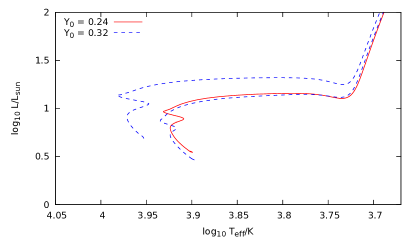
Figure 1: Evolution tracks for a $1.2\mathrm{M}_{\odot}$ helium-normal star (solid track) and a $1.2\mathrm{M}_{\odot}$ (upper dashed track) and a $1.05\mathrm{M}_{\odot}$ (lower dashed track) $Y_{0}=0.32$ star.

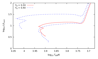
Figure 2: As figure (1) for $Y_{0}=0.4$. The lower dashed track is for a $0.9\mathrm{M}_{\odot}$ star.

A direct consequence of their higher luminosity is that a helium-rich star of a given mass has a considerably shorter main sequence lifetime than a helium normal star of the same mass. A helium-rich star with the same lifetime as a helium normal star will be less massive. The evolution tracks of such “coeval” stars are also much closer in terms of colour and luminosity (Figures 1 and 2). In other words, although it is true that helium-rich stars are brighter and bluer than normal stars for the same mass, this effect is much less significant when comparing populations of stars with the same age. This is the reason that a helium-rich population in a cluster shows up as a broadening (or splitting) of the main sequence rather than as an extension of the main sequence.

Helium-rich stars mimic helium normal stars of higher mass in other ways. For $Y_{0}=0.24$, a convective core appears on the main sequence above $M=1.1\mathrm{M}_{\odot}$, while for $Y_{0}=0.32$ an $M=1\mathrm{M_{\odot}}$ solar mass star already has a convective core. For $Y_{0}=0.4$ the convective core already develops for $M=0.9\mathrm{M_{\odot}}$.

The mass loss prescription (1) predicts a higher mass loss rate on the RGB for hotter stars, which means that the mass loss rate of helium enhanced stars is higher than that of helium normal stars. Nevertheless, the integrated mass loss on the RGB is lower for helium enhanced stars. This is due to the lower luminosity at the tip of the RGB, which is in turn due to the helium flash occurring at lower core mass. This reduces the integrated mass loss mainly because the mass loss rate is highest near the tip of the RGB and also because it shortens the RGB lifetime.

The lower core mass for helium ignition is due to an increased temperature at the base of the hydrogen burning shell. The easiest way to see why a higher helium abundance in the envelope leads to an increase of temperature in the core is by shell source homology (Refsdal & Weigert, 1970; Kippenhahn & Weigert, 1990). The temperature at the bottom of the hydrogen burning shell scales as

$$\frac{T_{\mathrm{shell}}}{\mu}\propto\frac{M_{\mathrm{c}}}{R_{\mathrm{c}}},$$ (2)

where the molecular weight $\mu$ is a suitable “typical” value in the burning shell. Because the core is degenerate there is a relation between $M_{\mathrm{c}}$ and $R_{\mathrm{c}}$, say $R_{\mathrm{c}}\propto M_{\mathrm{c}}^{-\alpha}$ with $\alpha>0$ ($\alpha=1/3$ for cold degenerate matter). Using primes to indicate a helium enhanced model, we have

$$\frac{T_{\mathrm{shell}}}{T^{\prime}_{\mathrm{shell}}}=\frac{\mu}{\mu^{\prime}}\left(\frac{M_{\mathrm{c}}}{M^{\prime}_{\mathrm{c}}}\right)^{1+\alpha},$$ (3)

so for the same core mass the helium enhanced model will have a higher temperature at the bottom of the burning shell ($\mu^{\prime}>\mu$), which implies a higher temperature in the core. An alternative approach that leads to the same conclusion is to apply the virial theorem for the core and consider the effect of changing the composition of the envelope (c.f. Kippenhahn & Weigert, 1990, $\S$ 30.5).

The lower mass loss on the RGB increases the mass on the horizontal branch for helium-rich stars of a given initial mass, but because of the difference in lifetime a coeval helium-rich horizontal branch star will actually be less massive than a helium normal star.

The core mass at the beginning of the tp-AGB is higher for helium enhanced stars of the same mass but also for helium enhanced stars of the same lifetime. Because of this we expect the white dwarf remnants of helium enhanced stars to be more massive than the remnants of helium normal stars. This is an interesting result but the implications of this for the white dwarf population in globular clusters are beyond the scope of this work.

4 Structure of the collision products

4.1 Lifetime and luminosity and colour functions

The structure and evolution of the collision products agrees very well with previous findings (Sills et al., 1997; Glebbeek & Pols, 2008), bearing in mind the differences between helium enhanced and helium normal stars discussed in the previous section.

As can be expected from the “entropy sorting” principle, the most helium-rich object will settle at the core of the collision product. Figure 3 shows the difference in the evolution tracks for an $M=0.6+0.4\mathrm{M}_{\odot}$ collision product with different helium abundances in the primaries: as long as at least one of the stars has $Y_{0}=0.24$, the evolution tracks look qualitatively the same, but brighter and bluer with increasing helium abundance in the interior.

The evolution track of a collision product resulting from $Y_{0}=0.24$ and $Y_{0}=0.32$ progenitors is intermediate between the evolution tracks of stars with the same mass but an initially uniform helium composition of $Y_{0}=0.24$ or $Y_{0}=0.32$. For parent stars of equal mass the evolution track is similar to that of a $Y_{0}=0.28$ star of the same mass although it is not as blue. The evolution of the core, and therefore the lifetime, more closely resembles that of a $Y_{0}=0.32$ star than that of a $Y_{0}=0.28$ star.

In previous work (Sills et al., 1997; Glebbeek & Pols, 2008) we showed that the core of the collision product is formed by the secondary, unless the primary has evolved sufficiently to reduce its central entropy below that of the secondary. This is slightly more complicated in the case of merging stars with different helium abundances. An unevolved star with a higher helium abundance will have a lower central entropy than an unevolved star of the same mass with a normal helium abundance. It will therefore tend to settle in the core of the collision product, which will resemble a more evolved star, or the collision product of more evolved parents. For instance, the result of an $M_{1}=0.6\mathrm{M}_{\odot},Y_{0}=0.24$ and an $M_{2}=0.6\mathrm{M}_{\odot},Y_{0}=0.32$ collision at $6\,000$ Myr resembles the collision product of $M_{1}=0.4\mathrm{M}_{\odot},Y_{0}=0.24$ and $M_{1}=0.8\mathrm{M}_{\odot},Y_{0}=0.24$ at $8\,000$ Myr.

In general, it is hard to predict which star will form the core of the collision product without looking at the structure of the two stars. It is still true that if the primary is sufficiently evolved, it will provide the core of the collision product even if the secondary started out with a higher helium content. However, it will need to be more evolved than in the situation where the secondary has the same helium content initially.

In either case, the lifetime of the collision product is reduced because its central helium abundance is higher than the situation where both stars had a normal helium abundance. This effect is exacerbated by the increase in the stars’ luminosity due to the higher helium abundance in the envelope.

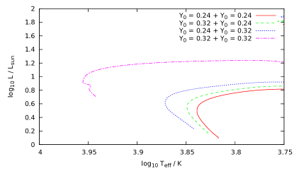
Figure 3: Evolution tracks for collisions between an $M=0.6\mathrm{M}_{\odot}$ and an $M=0.4\mathrm{M}_{\odot}$ star at 6000 Myr. The initial contraction phase is not shown for clarity.

4.2 Comparison with observed blue straggler populations

We compared the results of our models with the blue straggler populations in four galactic globular clusters: NGC 2808, NGC 1851, 5634 and NGC 6093 (M80), see Table 5. The latter cluster was also studied by Ferraro et al. (2003). Observations were taken from the HST WFPC2 database by Piotto et al. (2002) and blue stragglers were selected using the procedure of Leigh et al. (2007).

Table 5: Photometric parameters of our comparison clusters, taken from Harris (1996).

ID	Name	$E(B-V)$	$(m-M)$	[Fe/H]
NGC 1851		0.02	15.47	$-1.22$
NGC 2808		0.23	15.56	$-1.15$
NGC 5634		0.05	17.16	$-1.88$
NGC 6093	M80	0.18	15.56	$-1.75$

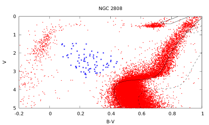
Figure 4: Colour-magnitide diagram for NGC 2808, showing the blue stragglers and a 12 Gyr isochrone for our adopted $E(B-V)$ and $m-M$ (solid line) as well as the $E(B-v)=0.23$ (dashed line).

These clusters were chosen because they all show different indications for multiple populations. In the case of NGC 2808, there is an observed splitting of the main sequence in at least three sequences (Piotto et al., 2007), which is attributed to the cluster population consisting of distinct sub-populations with a different helium abundance. It has become common to refer to these as “first generation” and “second generation” (or “third generation”), where the “first generation” refers to stars with a normal (low) helium abundance and “second generation” refers to the helium enriched population that (supposedly) formed later than the “first generation” out of polluted material.

For NGC 1851, the sub-giant branch is known to be split in at least two distinct populations (Saviane et al., 1998; Milone et al., 2008), which can be explained if there are two populations with different total CNO abundances (Cassisi et al., 2008; Ventura et al., 2009) but with the same helium abundance. Recently, Han et al. (2009) have presented evidence for a split giant branch in $U-I$ colours. Their interpretation of this is that there is a Helium enhanced population in NGC 1851 (with $Y=0.28$) that also has a slightly higher metallicity and they show that this would only show up as a split horizontal branch in $V-I$ colours.

Apart from the usual globular cluster abundance anomalies there is no photometric indication for a “second generation” in NGC 6093 or NGC 5634.

The scenario where some blue stragglers are formed through collisions between stars of different helium content should therefore apply only to the case of NGC 2808.

Comparing the photometry from Piotto et al. (2002) to that of Walker (1999), there appears to be a systematic colour shift $\Delta(B-V)\approx 0.1$ to the blue in the Piotto et al. (2002) data (before applying reddening corrections). The origin of this offset is unclear, but unless we correct for it we are unable to properly fit an isochrone to the data. In practice, we adopted the Piotto et al. (2002) data as it is available and determined an effective value of $E(B-V)=0.07$ for our isochrone. We use this value when comparing our models to the Piotto data.

The reddening for NGC 2808 is somewhat uncertain. Walker (1999) finds an overall value $E(B-V)=0.20\pm 0.02$, but notes that Schlegel et al. (1998) extinction maps indicate differential reddening across the cluster. Given the offset between the Piotto et al. (2002) and the Walker (1999) photometry and the error bars on the reddening, our effective value $E(B-V)=0.07$ for the Piotto data appears to be reasonable.

In order to compare our models with observations we calculate the colour and luminosity functions predicted by our models at an age of $12\mathrm{Gyr}$. The mass spacing of our model grid is not very fine and this results in very clear discrete jumps and gaps in the theoretical colour and luminosity distributions. To produce smoother distributions, we computed evolution sequences for collisions between stars with $31$ distinct masses between $0.4$ and $0.8$ (inclusive). For the masses that fall between those in our grid we interpolate between the neighbouring evolution tracks in a similar way to Pols et al. (1998).

In our model sets collisions only happen at discrete time intervals. In reality, collisions may happen at any time and for our simulated population we should generate collision models at intermediate times. We account for this by selecting for each evolution sequence the portion of the evolution track that falls within an age range of $12\,\mathrm{Gyr}\pm 500\,\mathrm{Myr}$. Every point along the evolution track is then assigned a weight

$$W_{i}=\Delta t_{i}\phi(m_{1})\phi(m_{2})\Psi(m_{1},m_{2},t_{\mathrm{coll}}),$$ (4)

where $\Delta t_{i}$ is the amount of time spent in the vicinity of the current point, $\phi(m)\propto m^{-\alpha}$ is the initial mass function of Kroupa (2001) and $\Psi(m_{1},m_{2},t_{\mathrm{coll}})$ is the collision probability for star 1 and star 2 at the time of collision $t_{\mathrm{coll}}$, which we take to be constant for simplicity. For model sets D and E the relative abundance of the different populations is important. We have taken all populations to be equally abundant, so that for model set D mixed $Y_{0}=0.24$ and $Y_{0}=0.32$ collisions are as likely as collisions between stars with the same helium content.

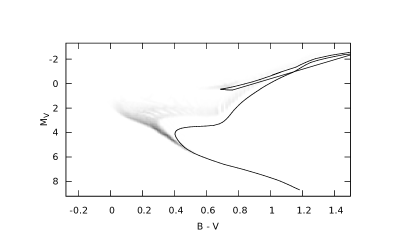
Figure 5: Theoretical colour-magnitude diagram for $Y_{0}=0.24$ and $Z=0.001$ at 12 $\mathrm{Gyr}$. The solid line is a single star isochrone.

The evolution tracks are then binned in the $B-V$ vs. $M_{\mathrm{V}}$ plane with the value of each bin being the sum of the weights $W_{i}$ of evolution tracks that pass through it. The width of our bins is $0.1$ in $M_{\mathrm{V}}$ and $0.089$ in $B-V$. To convert between theoretical $\log g$, $\log L$ and $T_{\mathrm{eff}}$ to observational $M_{\mathrm{V}}$ and $B-V$ we made use of the spectral library by Lejeune et al. (1997, 1998). The resulting colour-magnitude diagram for $Y_{0}=0.24$ is shown in Figure 5 along with a $Y_{0}=0.24$ isochrone. There are some gaps in the shading in the Hertzsprung gap between the main sequence and the giant branch where our binning method misses the stars as the evolve quickly through this region. Because the time spent in this region of the colour-magnitude diagram is small anyway, the weight $W_{i}$ at these points is also small and the presence of these gaps does not affect the results of our comparison.

The collision products detach from the zero-age main sequence around $B-V=0.5$ and fill up the blue straggler region above and to the blue of the main sequence turn-off. The collision product giant branch appears just to the blue of the normal single star giant branch and the horizontal branch is slightly bluer and brighter than the normal single star horizontal branch.

Observationally, blue stragglers are selected by drawing a selection box in the colour magnitude diagram, with cut-offs at the low luminosity end to separate the blue stragglers from the main sequence and at the high luminosity end to separate the blue stragglers from the horizontal branch. See Leigh et al. (2007) for a description of an algorithm to define these selection boxes consistently between different clusters. In some cases (most notably NGC 6093 and NGC 1851) the resulting selection box includes one or two blue stragglers that are substantially ($>0.1\mathrm{dex}$) fainter than the rest. This strongly affects the shape of the luminosity function at the low-luminosity end and we have redrawn our selection box to reject these stars from both the observations and our models.

To compare our models to the observations, we have selected the blue stragglers from our models using the same selection box as was used to select the observed blue stragglers. These selection boxes vary slightly from cluster to cluster, so that the range of colours and luminosities spanned by the blue stragglers also differs slightly from cluster to cluster.

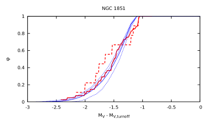
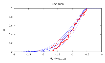
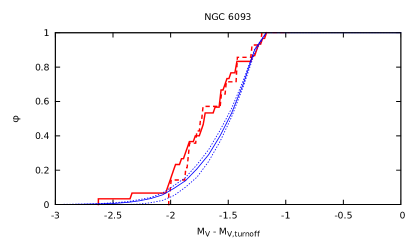
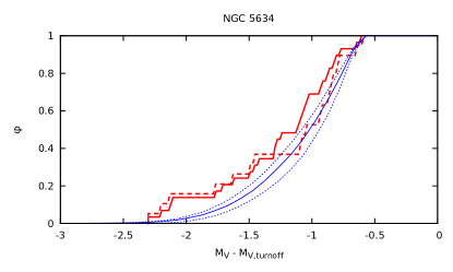
Figure 6: Cumulative luminosity functions $\varphi$ for the observed blue straggler populations in the whole cluster (thick red solid line), in the cluster core (thick red dashed line) and the luminosity function for the collision models (thin blue lines). The solid line is for model set D, the dotted lines are for $Y_{0}=0.40$ (model set C), $Y_{0}=0.24$ (model set A) and $Y_{0}=0.32$ (model set B) respectively from left to right.

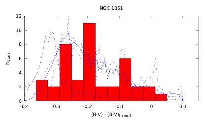
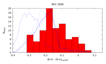
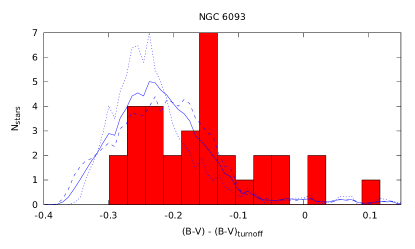
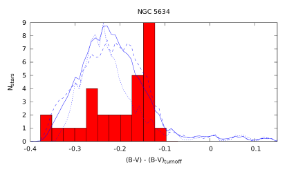
Figure 7: Total $B-V$ colour distributions of the observed blue straggler populations (histogram) and the colour distributions for the collision models (curves). The solid line represents model set D. The dashed, dotted and dash-dotted lines represent model sets A – C respectively.

We compare our $Z=0.001$ ($[\mathrm{Fe}/\mathrm{H}]=-1.3$) models with NGC 1851 and NGC 2808, which have a slightly higher metallicity (Table 5). Our $Z=0.0003$ ($[\mathrm{Fe}/\mathrm{H}]=-1.82$) models are compared with NGC 5634 and NGC 6093, which straddle this metallicity.

The (observed and model) blue straggler luminosity functions are shown in Figure 6 and the colour distributions are shown in Figure 7. Table 6 gives the probability that the observed luminosity function is drawn from model sets A, B, C, D or E (defined in Table 1), as determined by a standard K-S test. The listed value $p_{0}$ is the probability using the observed value for $M-m$. The value $p^{\prime}$ was derived by treating the distance modulus as a free parameter that was then derived from fitting to the data. The difference between the observed value of $M-m$ (listed in Table 5) and the best fitting value for $M-m$ is listed as $\Delta(M-m)$. We will discuss each of the clusters in turn.

Table 6: K-S test probabilities comparing the theoretical and observed blue straggler luminosity functions for the entire cluster.

Cluster	Model set	$p_{0}$	$p^{\prime}$	$\Delta(M-m)$
NGC 1851	A	0.45	0.75	$+0.03$
	B	0.13	0.30	$-0.02$
	C	0.43	0.90	$+0.05$
	D	0.45	0.61	$+0.01$
	E	0.43	0.66	$+0.02$
NGC 2808	A	0.15	0.82	$+0.09$
	B	0.19	0.45	$-0.09$
	C	0.03	0.73	$+0.14$
	D	0.62	0.89	$+0.03$
	E	0.45	0.88	$+0.05$
NGC 5634	A	0.35	0.75	$-0.12$
	B	$<10^{-3}$	0.52	$-0.20$
	D	0.05	0.69	$-0.17$
NGC 6093	A	0.12	0.40	$-0.04$
	B	0.01	0.18	$-0.07$
	D	0.04	0.27	$-0.06$

4.2.1 NGC 1851

For NGC 1851 most of our model luminosity functions fit the observations about equally well ($p\sim 0.45$) with the exception of the helium enhanced $Y_{0}=0.32$ models (model set B). If we allow for a shift in $M-m$ then the best fits are for model set C ($p=0.90$) and A ($p=0.75$).

The high luminosity end of the distribution best fits the pure $Y_{0}=0.24$ models (model set A), with $p>0.999$ if we only select blue stragglers brighter than $M_{\mathrm{V}}=2.7$. We can match the fainter end of the luminosity function, which then matches best with the $Y_{0}=0.4$ collision models (model set C) with $p=0.81$. However, in that case our models do not match the high luminosity end of the luminosity function. The luminosity function for the core is clearly brighter than for the cluster as a whole, which could be a signature of mass segregation. However, the number of stars is small so it is hard to draw any firm conclusions.

The predicted colour distribution from our models gives a tolerable fit to the observations. We predict more stars between $B-V=0.2$ and $0.3$, but the number of observed stars in this colour range is small. The predicted location of the peak in the colour distribution may be somewhat too blue. A K-S test for the cumulative colour distribution functions is not very conclusive. Model set C is too blue on average and has the lowest probability, of $0.52$. The next lowest probability is $0.97$ for model set E. All other model sets have probabilities $>0.99$.

Taking into account both colour and luminosity, model set A ($Y_{0}=0.24$) is most consistent with observations for NGC 1851.

4.2.2 NGC 2808

For NGC 2808 the best agreement ($p=0.62$) is obtained for a mixed population of collision products involving $Y_{0}=0.24$ and $Y_{0}=0.32$ stars (model set D), although good agreement with the pure $Y_{0}=0.24$ and a mixture of all collision products can also be obtained by allowing for a shift in the distance modulus. The combination of $Y_{0}=0.24$ and $Y_{0}=0.32$ marginally remains in best agreement with the observations, however. Interestingly enough, the high-luminosity end of the luminosity function is in better agreement with the pure $Y_{0}=0.32$ collisions, which is in line with expectations.

The core luminosity function seems to fit slightly better with a pure $Y_{0}=0.24$ component for luminosities that are one magnitude brighter than the turnoff, which is compatible with mass segregation since stars of $Y_{0}=0.24$ are expected to be more massive than stars with $Y_{0}=0.32$ on average.

The range of colours spanned by our collision models agrees well with the observations, and both place the peak between $\Delta(B-V)=-0.2$ and $-0.1$. The observations may fall off more quickly on the blue side, but the difference is within the expected error based on the number of observed stars in the colour bins. On the other hand, the observations clearly show an excess of blue stragglers to the red of $\Delta(B-V)=-0.1$. In our models the stars in this colour range are post-main sequence objects that are in the Hertzsprung gap. Similar discrepancies between models and observations have been noted before (e.g. Sills et al., 2000). Extra mixing, for instance due to rapid rotation, offers one possible way to extend the lifetime of stars in this region. Convective overshooting, as noted before, is ineffective in removing this discrepancy. Another possibility is that at least some of the stars in this region are unresolved binaries.

A K-S test of the cumulative colour distribution gives about equal probability of $0.70$ to both model sets B and D, followed by model set A with a probability of $0.62$. The pure $Y_{0}=0.4$ models (model set C) has a probability $<0.001$. Combining both the colour and luminosity information, our model set D best describes the blue stragglers in NGC 2808.

4.2.3 NGC 6093

None of our luminosity functions fit particularly well. The best fitting model is model set A, although model set D is not much worse. By varying the distance modulus, model set A can be made to fit a bit better, while the fit for model set D does not improve significantly.

The colour distributions for the different model sets are all very similar. The observations show a peak that is $0.15$ magnitudes bluer than the turnoff. As with NGC 2808, there are more observed blue stragglers redward of $\Delta(B-V)=-0.1$ than predicted by our models. By contrast, no blue stragglers are observed blueward of $\Delta(B-V)=-0.3$. The $Y_{0}=0.24$ models fit slightly better ($p=0.39$) than the mixed $Y_{0}=0.24;0.32$ models ($p=0.25$) but the picture is not very clear.

4.2.4 NGC 5634

Again, none of our models fit very well. Model set A ($Y_{0}=0.24$) gives the best agreement with the observations, although model set D is also not a bad fit if we vary the distance modulus. The theoretical luminosity function falls off perhaps a little too quickly for higher luminosities. The colour distributions are not very different for the three model sets and all match about equally well. The observations show a peak 0.1 dex bluer than the turnoff that is not present in the models.

4.3 Late evolutionary phases

The late (post-main sequence) evolution of collision products is interesting for two reasons. First of all it allows us to test our understanding of the subsequent evolution of collision products by comparing the observed distributions and properties of evolved blue stragglers (post-blue stragglers) with the models. Second of all, it may allow us to probe the dynamical history of the cluster over a longer time interval than can be accomplished with the blue stragglers alone.

The most promising post-main sequence evolutionary phase to identify stellar collision products is during core helium burning. Observationally, the collision products are then expected to lie above the horizontal branch (Renzini & Fusi Pecci, 1988; Fusi Pecci et al., 1992; Ferraro et al., 1999; Sills et al., 2009).

We can derive a selection box for evolved collision products by using the evolution models. The first step is to determine the minimum and maximum values of $M_{V}$ and $B-V$ during core helium burning for all of our collision models. These define a selection box in the colour-magnitude diagram that contains the core helium burning phase of all our collision products. However, for some models this selection box will now encompass more than just the core helium burning phase. Due to the difference in helium content, the colour of the giant branch is different for different models in our set. We therefore restrict our selection box so that it does not overlap with the red giant branch in any of our models. We also impose a cut to remove the cluster horizontal branch. This way, we aim to select only stars that are unambiguously evolved blue stragglers. Because we have restricted the selection box, we will not capture all of the core helium burning phase for all collision products, and we may miss $\sim 20\%$ of the core He burning collision products by using this narrower selection box. In the $\log_{10}T_{\mathrm{eff}}$ / $\log_{10}L/L_{\odot}$ plane our selection box is very similar to that of Sills et al. (2009).

We can define a selection box for the AGB in the same way as for the core helium burning phase, but this selection box turns out to be very narrow. Since the expected ratio of blue stragglers to AGB post-blue stragglers is also very high, $\sim 1000$, it is virtually impossible to compare with observations. Therefore, we only compare the ratio of blue stragglers to core helium burning post-blue stragglers.

The predicted ratio of blue stragglers to evolved blue stragglers is typically $20$ – $50$. Observationally, the ratios are about $10$, but there are only a few stars in the evolved blue straggler selection box and numbers are very sensitive to whether any particular star is classified as an evolved blue straggler or not.

A reasonable agreement between models and observations was reached by Sills et al. (2009) based on the average of the horizontal branch and main sequence lifetimes of their collision products, as long as they selected only the brighter (more massive) collision products. Our approach differs from theirs in two respects: first of all we calculate a population of collision products where each collision product is assigned a weight that depends on the IMF probability of the parent stars as opposed to taking a straight average. Second of all we calculate our population ratios, for both the models and the observations, based on selection boxes in the colour magnitude diagram, not on the relative duration of the evolution phases themselves.

The first of these has the effect of giving more importance to the lower mass collision products, which will tend to increase the predicted ratios. The effect of using selection boxes that will only capture part of the evolution rather than comparing the lifetimes directly will similarly tend to increase the blue straggler to post-blue straggler ratio. Neither of these effects should affect the comparison between our models and the observations, however, because blue stragglers and evolved blue stragglers are selected consistently between the observations and in the models – if the models reflect the observed population, then these population ratios should come out the same as long as the selection criteria are the same. However, the small number of observed stars that actually fall within our selection box make it hard to draw any firm conclusions from this comparison.

5 Summary and Discussion

We present new evolution calculations for stellar collision products, where we have allowed the progenitor stars to have a different helium abundance.

Our collision models do a reasonable job of reproducing the observed blue straggler luminosity function and colour distribution. We predict, perhaps, too few blue stragglers at the red edge of the observed distribution. For NGC 1851, the best agreement is obtained for a single population of helium normal stars ($Y_{0}=0.24$) while for NGC 2808 the best fit is obtained with a population of mixed $Y_{0}=0.24$ and $Y_{0}=0.32$ stars. These results are what we would expect in light of observations of multiple populations in these clusters. A lower metallicity set of models agrees with NGC 6093 and NGC 5634 in the sense that the best fitting models are those without a helium enhanced population. The observed population ratios of blue stragglers to evolved blue stragglers is larger than is seen in the observations, but the number of observed evolved blue straggler candidates is small.

Recently, Han et al. (2009) reported the presence of two distinct populations in NGC 1851, one helium normal and one helium enhanced ($Y=0.28$). However, they also report that the helium-rich population has a higher metallicity, which offsets the colour changes due to helium enhancement, at least in $V-I$ colours. Since all our models have the same metallicity, there is no corresponding compensation for the shift in colour due to helium enhancement. To compare our models more directly we would need to allow for a similar shift in metallicity.

Although the agreement between our models and the observations is reasonable, the agreement is not perfect and the models presented here are not complete. There are two obvious improvements that can be made. The first of these has to do with the blue straggler formation rate, which we have effectively taken to be constant and independent of the helium abundances of the two colliding stars. By allowing the collision rate $\Psi$ in (4) to vary with $t_{\mathrm{coll}}$ we have more freedom in shaping the colour and luminosity functions – in fact, if we want to use blue stragglers (and possibly evolved blue stragglers) to learn about the dynamical history of their host cluster, then it is essential that we allow this factor to vary. Simulations of clusters hosting multiple populations, like those of D’Ercole et al. (2008) may serve as a guide for how this should be done. Ideally, the collision rate should be directly determined from dynamical simulations of cluster evolution. A software environment that might be especially suited for this task is the MUSE software package, which is in active development (Portegies Zwart et al., 2009).

The second improvement that can (and should) be made is that we should consider binaries in addition to single star models. For the blue stragglers, this is an obvious addition because binary mass transfer is an alternative scenario for blue straggler production (e.g. Chen & Han, 2009). However, binaries are also important in another respect: observationally, it is not possible to distinguish the light of the two stars in a binary system, which may place the system in an unusual point in the colour magnitude diagram that is hard to reproduce with single star evolution tracks. This becomes especially important when we look for evolved blue stragglers because a blend of a horizontal branch star and a red giant may appear in the same region of the colour-magnitude diagram as the evolved blue stragglers. Such unresolved binaries can be recognised by multi-wavelength photometry because the colour of the unresolved binary will not change in the same way as that of a single star, and the binary will move to a different region of the colour-magnitude diagram: a normal star will stay close to other stars of a similar spectral type, but an unresolved binary will move closer to the position of one of its unresolved components.

Evolved blue stragglers offer an interesting possibility to test our understanding of blue straggler evolution, but because the number of observed post-blue straggler candidates is small it is especially important to understand how this region of the colour magnitude diagram may be influenced by the presence of binaries. Both normal binary interaction and collisions can increase the actual number of stars in the evolved blue straggler region without increasing the number of blue stragglers. Unstable binary mass transfer from a red giant to an unevolved main sequence star companion can lead to a spiral in and merger of the two stars if the envelope is not ejected. A collision with a red giant will have a similar result. The red giant core is likely to remain intact during the merger so the merger product will still have a degenerate helium core and evolve like a more massive red giant. Such a merger would show up as an “evolved blue straggler” despite never having been a blue straggler itself.

Our population models are consistent with observations of multiple populations in the sense that helium enhanced model sets fit best with clusters (in particular, NGC 2808) where helium enhancement has been inferred from the observations. We hope that with the inclusion of a population of binaries, population models such as we have presented in this paper could be used not only to test our understanding of cluster dynamics but also to get a better handle on the nature of the multiple populations that are now observed in star clusters. Future cluster simulations that include an accurate treatment of the evolution of stellar collision products as well as multiple populations will be an important diagnostic tool and we plan to make our models available for such a study.

References

- Alexander & Ferguson (1994) Alexander D. R., Ferguson J. W., 1994, ApJ, 437, 879
- Anders & Grevesse (1989) Anders E., Grevesse N., 1989, Geochim. Cosmochim. Acta, 53, 197
- Angulo et al. (1999) Angulo C., Arnould M., Rayet M., et al., 1999, Nuclear Physics A, 656, 3
- Bedin et al. (2004) Bedin L. R., Piotto G., Anderson J., Cassisi S., King I. R., Momany Y., Carraro G., 2004, ApJL, 605, L125
- Böhm-Vitense (1958) Böhm-Vitense E., 1958, Zeitschrift fur Astrophysik, 46, 108
- Buchler & Yueh (1976) Buchler J. R., Yueh W. R., 1976, ApJ, 210, 440
- Campbell & Lattanzio (2008) Campbell S. W., Lattanzio J. C., 2008, A&A, 490, 769
- Cassisi et al. (2008) Cassisi S., Salaris M., Pietrinferni A., Piotto G., Milone A. P., Bedin L. R., Anderson J., 2008, ApJL, 672, L115
- Chen & Han (2004) Chen X., Han Z., 2004, MNRAS, 355, 1182
- Chen & Han (2008) Chen X., Han Z., 2008, MNRAS, 384, 1263
- Chen & Han (2009) Chen X., Han Z., 2009, MNRAS, 395, 1822
- D’Antona et al. (2005) D’Antona F., Bellazzini M., Caloi V., Pecci F. F., Galleti S., Rood R. T., 2005, ApJ, 631, 868
- de Mink et al. (2009) de Mink S. E., Pols O. R., Langer N., Izzard R. G., 2009, A&A, 507, L1
- Dearborn et al. (2006) Dearborn D. S. P., Lattanzio J. C., Eggleton P. P., 2006, ApJ, 639, 405
- Decressin et al. (2007) Decressin T., Meynet G., Charbonnel C., Prantzos N., Ekström S., 2007, A&A, 464, 1029
- D’Ercole et al. (2008) D’Ercole A., Vesperini E., D’Antona F., McMillan S. L. W., Recchi S., 2008, MNRAS, 391, 825
- Eggleton (1971) Eggleton P. P., 1971, MNRAS, 151, 351
- Eggleton (1972) Eggleton P. P., 1972, MNRAS, 156, 361
- Eldridge & Tout (2004) Eldridge J. J., Tout C. A., 2004, MNRAS, 348, 201
- Ferraro et al. (1999) Ferraro F. R., Paltrinieri B., Rood R. T., Dorman B., 1999, ApJ, 522, 983
- Ferraro et al. (2003) Ferraro F. R., Sills A., Rood R. T., Paltrinieri B., Buonanno R., 2003, ApJ, 588, 464
- Ferraro et al. (2004) Ferraro F. R., Sollima A., Pancino E., Bellazzini M., Straniero O., Origlia L., Cool A. M., 2004, ApJL, 603, L81
- Formicola et al. (2004) Formicola A., Imbriani G., Costantini H., et al., 2004, Physics Letters B, 591, 61
- Fujimoto et al. (1990) Fujimoto M. Y., Iben I. J., Hollowell D., 1990, ApJ, 349, 580
- Fusi Pecci et al. (1992) Fusi Pecci F., Ferraro F. R., Corsi C. E., Cacciari C., Buonanno R., 1992, AJ, 104, 1831
- Glebbeek & Pols (2008) Glebbeek E., Pols O. R., 2008, A&A, 488, 1017
- Glebbeek et al. (2008) Glebbeek E., Pols O. R., Hurley J. R., 2008, A&A, 488, 1007
- Gratton et al. (2004) Gratton R., Sneden C., Carretta E., 2004, ARA&A, 42, 385
- Han et al. (2009) Han S., Lee Y., Joo S., Sohn S. T., Yoon S., Kim H., Lee J., 2009, ApJL, 707, L190
- Härm & Schwarzschild (1966) Härm R., Schwarzschild M., 1966, ApJ, 145, 496
- Harris (1996) Harris W. E., 1996, AJ, 112, 1487
- Herwig et al. (2006) Herwig F., Austin S. M., Lattanzio J. C., 2006, Phys. Rev. C, 73, 025802
- Iben (1975) Iben Jr. I., 1975, ApJ, 196, 525
- Iglesias & Rogers (1996) Iglesias C. A., Rogers F. J., 1996, ApJ, 464, 943
- Kippenhahn et al. (1980) Kippenhahn R., Ruschenplatt G., Thomas H.-C., 1980, A&A, 91, 175
- Kippenhahn & Weigert (1990) Kippenhahn R., Weigert A., 1990, Stellar Structure and Evolution. Stellar Structure and Evolution, XVI, 468 pp. 192 figs.. Springer-Verlag Berlin Heidelberg New York. Also Astronomy and Astrophysics Library
- Knigge et al. (2009) Knigge C., Leigh N., Sills A., 2009, Nature, 457, 288
- Kroupa (2001) Kroupa P., 2001, MNRAS, 322, 231
- Leigh et al. (2007) Leigh N., Sills A., Knigge C., 2007, ApJ, 661, 210
- Leigh et al. (2008) Leigh N., Sills A., Knigge C., 2008, ApJ, 678, 564
- Lejeune et al. (1997) Lejeune T., Cuisinier F., Buser R., 1997, AAPS, 125, 229
- Lejeune et al. (1998) Lejeune T., Cuisinier F., Buser R., 1998, AAPS, 130, 65
- Lombardi et al. (1995) Lombardi Jr. J. C., Rasio F. A., Shapiro S. L., 1995, ApJL, 445, L117
- Lombardi et al. (2002) Lombardi Jr. J. C., Warren J. S., Rasio F. A., Sills A., Warren A. R., 2002, ApJ, 568, 939
- Milone et al. (2008) Milone A. P., Bedin L. R., Piotto G., Anderson J., King I. R., Sarajedini A., Dotter A., Chaboyer B., Marín-Franch A., Majewski S., Aparicio A., Hempel M., Paust N. E. Q., Reid I. N., Rosenberg A., Siegel M., 2008, ApJ, 673, 241
- Mocák et al. (2009) Mocák M., Müller E., Weiss A., Kifonidis K., 2009, A&A, 501, 659
- Pancino et al. (2000) Pancino E., Ferraro F. R., Bellazzini M., Piotto G., Zoccali M., 2000, ApJL, 534, L83
- Piotto et al. (2007) Piotto G., Bedin L. R., Anderson J., King I. R., Cassisi S., Milone A. P., Villanova S., Pietrinferni A., Renzini A., 2007, ApJL, 661, L53
- Piotto et al. (2002) Piotto G., King I. R., Djorgovski S. G., Sosin C., Zoccali M., Saviane I., De Angeli F., Riello M., Recio-Blanco A., Rich R. M., Meylan G., Renzini A., 2002, A&A, 391, 945
- Piotto et al. (2005) Piotto G., Villanova S., Bedin L. R., Gratton R., Cassisi S., Momany Y., Recio-Blanco A., Lucatello S., Anderson J., King I. R., Pietrinferni A., Carraro G., 2005, ApJ, 621, 777
- Pols et al. (1998) Pols O. R., Schroder K.-P., Hurley J. R., Tout C. A., Eggleton P. P., 1998, MNRAS, 298, 525
- Pols et al. (1995) Pols O. R., Tout C. A., Eggleton P. P., Han Z., 1995, MNRAS, 274, 964
- Portegies Zwart et al. (2009) Portegies Zwart S., McMillan S., Harfst S., et al., 2009, New Astronomy, 14, 369
- Refsdal & Weigert (1970) Refsdal S., Weigert A., 1970, A&A, 6, 426
- Renzini & Fusi Pecci (1988) Renzini A., Fusi Pecci F., 1988, ARA&A, 26, 199
- Sandage (1953) Sandage A. R., 1953, AJ, 58, 61
- Saviane et al. (1998) Saviane I., Piotto G., Fagotto F., Zaggia S., Capaccioli M., Aparicio A., 1998, A&A, 333, 479
- Schlegel et al. (1998) Schlegel D. J., Finkbeiner D. P., Davis M., 1998, ApJ, 500, 525
- Schröder & Cuntz (2005) Schröder K., Cuntz M., 2005, ApJL, 630, L73
- Schröder & Cuntz (2007) Schröder K., Cuntz M., 2007, A&A, 465, 593
- Sills et al. (2005) Sills A., Adams T., Davies M. B., 2005, MNRAS, 358, 716
- Sills et al. (2000) Sills A., Bailyn C. D., Edmonds P. D., Gilliland R. L., 2000, ApJ, 535, 298
- Sills et al. (2009) Sills A., Karakas A., Lattanzio J., 2009, ApJ, 692, 1411
- Sills et al. (1997) Sills A., Lombardi Jr. J. C., Bailyn C. D., Demarque P., Rasio F. A., Shapiro S. L., 1997, ApJ, 487, 290
- Stancliffe (2006) Stancliffe R. J., 2006, MNRAS, 370, 1817
- Stancliffe et al. (2007) Stancliffe R. J., Glebbeek E., Izzard R. G., Pols O. R., 2007, A&A, 464, L57
- Ventura et al. (2009) Ventura P., Caloi V., D’Antona F., Ferguson J., Milone A., Piotto G., 2009, ArXiv e-prints
- Ventura & D’Antona (2005) Ventura P., D’Antona F., 2005, ApJL, 635, L149
- Ventura et al. (2002) Ventura P., D’Antona F., Mazzitelli I., 2002, A&A, 393, 215
- Ventura et al. (2001) Ventura P., D’Antona F., Mazzitelli I., Gratton R., 2001, ApJL, 550, L65
- Walker (1999) Walker A. R., 1999, AJ, 118, 432