Opportunistic Interference Mitigation Achieves Optimal Degrees-of-Freedom in Wireless Multi-cell Uplink Networks

Abstract

We introduce an opportunistic interference mitigation (OIM) protocol, where a user scheduling strategy is utilized in $K$-cell uplink networks with time-invariant channel coefficients and base stations (BSs) having $M$ antennas. Each BS opportunistically selects a set of users who generate the minimum interference to the other BSs. Two OIM protocols are shown according to the number $S$ of simultaneously transmitting users per cell: opportunistic interference nulling (OIN) and opportunistic interference alignment (OIA). Then, their performance is analyzed in terms of degrees-of-freedom (DoFs). As our main result, it is shown that $KM$ DoFs are achievable under the OIN protocol with $M$ selected users per cell, if the total number $N$ of users in a cell scales at least as $\text{SNR}^{(K-1)M}$. Similarly, it turns out that the OIA scheme with $S$($<M$) selected users achieves $KS$ DoFs, if $N$ scales faster than $\text{SNR}^{(K-1)S}$. These results indicate that there exists a trade-off between the achievable DoFs and the minimum required $N$. By deriving the corresponding upper bound on the DoFs, it is shown that the OIN scheme is DoF-optimal. Finally, numerical evaluation, a two-step scheduling method, and the extension to multi-carrier scenarios are shown.

I Introduction

Interference between wireless links has been taken into account as a critical problem in communication systems. Especially, there exist three categories of the conventional interference management in multi-user wireless networks: decoding and cancellation, avoidance (i.e., orthogonalization), and averaging (or spreading). To consider both intra-cell and inter-cell interferences of wireless cellular networks, a simple infinite cellular multiple-access channel (MAC) model, referred to as the Wyner’s model, was characterized and then its achievable throughput performance was analyzed in [1, 2, 3, 4]. Moreover, joint processing strategy among multi-cells was developed in a Wyner-like cellular model in order to efficiently manage the inter-cell interferences [5, 6]. Such cooperation among cells can be taken into account as another important interference management scheme. Even if the work in [1, 2, 3, 4, 5, 6] leads to remarkable insight into complex and analytically intractable practical cellular environments, the model under consideration is hardly realistic.

Recently, as an alternative approach to show Shannon-theoretic limits, interference alignment (IA) was proposed by fundamentally solving the interference problem when there are two communication pairs [7]. It was shown in [8] that the IA scheme can achieve the optimal degrees-of-freedom (DoFs), which are equal to $K/2$, in the $K$-user interference channel with time-varying channel coefficients. The basic idea of the scheme is to confine all the undesired interference from other communication links into a pre-defined subspace, whose dimension approaches that of the desired signal space. Hence, it is possible for all users to achieve one half of the DoFs that we could achieve in the absence of interference. Since then, interference management schemes based on IA have been further developed and analyzed in various wireless network environments: multiple-input multiple-output (MIMO) interference network [9, 10], X network [11, 12], and cellular network [13, 14, 15]. However, the conventional IA schemes [8, 10, 16] require global channel state information (CSI) including the CSI of other communication links. Furthermore, a huge number of dimensions based on time/frequency expansion are needed to achieve the optimal DoFs [8, 10, 11, 12, 13, 16]. These constraints need to be relaxed in order to apply IA to more practical systems. In [9], a distributed IA scheme was constructed for the MIMO interference channel with time-invariant coefficients. It requires only local CSI at each node that can be acquired from all received channel links via pilot signaling, and thus is more feasible to implement than the original one [8]. However, a great number of iterations should be performed until designed transmit/receive beamforming (BF) vectors converge prior to data transmission.

Now we would like to consider practical wireless uplink networks with $K$-cells, each of which has $N$ users. IA for $K$-cell uplink networks was first proposed in [13], where the interference from other cells is aligned into a multi-dimensional subspace instead of one dimension. This scheme also has practical challenges including a dimension expansion to achieve the optimal DoFs.

In the literature, there are some results on the usefulness of fading in single-cell downlink broadcast channels, where one can obtain a multi-user diversity (MUD) gain as the number of mobile users is sufficiently large: opportunistic scheduling [17], opportunistic BF [18], and random BF [19]. More efficient opportunistic interference management strategy [20, 21], which requires less feedback overhead than that in [19], has been developed in broadcast channels, where similarly as in our study, the minimum number of users needed for achieving target DoFs has been analyzed. Scenarios exploiting the MUD gain have also been studied in cooperative networks by applying an opportunistic two-hop relaying protocol [22] and an opportunistic routing [23], and in cognitive radio networks with opportunistic scheduling [24, 25]. In addition, recent results [16, 26] have shown how to utilize the opportunistic gain when we have a large number of channel realizations. More specifically, to amplify signals and cancel interference, the idea of opportunistically pairing complementary channel instances has been studied in interference networks [16] and multi-hop relay networks [26]. In cognitive radio environments [27, 28, 29], opportunistic spectrum sharing was introduced by allowing the secondary users to share the radio spectrum originally allocated to the primary users via transmit adaptation in space, time, or frequency.

In this paper, we introduce an opportunistic interference mitigation (OIM) protocol for wireless multi-cell uplink networks. The scheme adopts the notion of MUD gain for performing interference management. The opportunistic user scheduling strategy is presented in $K$-cell uplink environments with time-invariant channel coefficients and base stations (BSs) having $M$ receive antennas. In the proposed OIM scheme, each BS opportunistically selects a set of users who generate the minimum interference to the other BSs, while in the conventional opportunistic algorithms [17, 18, 19], users with the maximum signal strength at the desired BS are selected for data transmission. Specifically, two OIM protocols are proposed according to the number $S$ of simultaneously transmitting users per cell: opportunistic interference nulling (OIN) and opportunistic interference alignment (OIA) protocols. For the OIA scheme, each BS broadcasts its pre-defined interference direction, e.g., a set of orthonormal random vectors, to all the users in other cells, whereas for the OIN scheme, no broadcast is needed at each BS. Each user computes the amount of its generating interference, affecting the other BSs, and feeds back it to its home cell BS.

Their performance is then analyzed in terms of achievable DoFs (also known as capacity pre-log factor or multiplexing gain). It is shown that $KM$ DoFs are achievable under the OIN protocol with $M$ selected users per cell, while the OIA scheme with $S$ selected users, whose number is smaller than $M$, achieves $KS$ DoFs. As our main result, we analyze the scaling condition between the number $N$ of per-cell users the received signal-to-noise ratio (SNR) under which our achievability result holds in $K$-cell networks, each of which has $N$ users. More specifically, we show that the aforementioned DoFs are achieved asymptotically, provided that $N$ scales faster than $\text{SNR}^{(K-1)M}$ and $\text{SNR}^{(K-1)S}$ for the OIN and OIA protocols, respectively. From the result, it is seen that there exists a fundamental trade-off between the achievable DoFs and the minimum required number $N$ of users per cell, based on the two proposed schemes. In addition, we derive an upper bound on the DoFs in $K$-cell uplink networks. It is shown that the upper bound always approaches $KM$ regardless of $N$ and thus the OIN scheme achieves the optimal DoFs asymptotically with the help of the opportunism.

Some important aspects are discussed as follows. To validate the OIA scheme, computer simulations are performed—the amount of interference leakage is evaluated as in [9, 30]. In addition, the conventional opportunistic mechanism exploiting the MUD gain in the literature [17, 18, 19] inspires us to introduce a two-step scheduling strategy with a slight modification. We show that a logarithmic gain can further be obtained, similarly as in [17, 18, 19], while the full DoFs are maintained. Extension to multi-carrier systems of our achievability result is also taken into account. Finally, the proposed scheme is also compared with the existing methods which can also asymptotically achieve the optimal DoFs in cellular uplink networks.

As in [9], the OIM protocol basically operates with local CSI and no time/frequency expansion, thereby resulting in easier implementation. No iteration is also needed prior to data transmission. The scheme thus operates as a decentralized manner which does not involve joint processing among all communication links.

The rest of this paper is organized as follows. In Section II, we introduce the system and channel models. In Section III, the OIM technique is proposed for cellular networks and its achievability in terms of DoFs is also analyzed. Section IV shows an upper bound on the DoFs. Numerical evaluation, the two-step scheduling method, extension to multi-carrier scenarios, and comparison with the existing methods are shown in Section V. Finally, we summarize the paper with some concluding remark in Section VI.

Throughout this paper, the superscripts $T$, $H$, and $\dagger$ denote the transpose, conjugate transpose, and pseudo-inverse, respectively, of a matrix (or a vector). $\mathbb{C}$, $\|\cdot\|$, $\mathbf{I}_{n}$, $\lambda_{\operatornamewithlimits{min}}(\cdot)$, $\mathbb{E}[\cdot]$, and $\text{diag}(\cdot)$ indicate the field of complex numbers, $L_{2}$-norm of a vector, the identity matrix of size $n\times n$, the smallest eigenvalue of a matrix, and the statistical expectation, and the vector consisting of the diagonal elements of a matrix, respectively.

II System and Channel Models

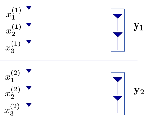
Figure 1: The IMAC model with $K$=2, $N=3$, and $M=2$.

Consider the interfering MAC (IMAC) model in [13], which is one of multi-cell uplink scenarios, to describe practical cellular networks. As illustrated in Fig. 1, there are multiple cells, each of which has multiple mobile users. The example for $K=2$, $N=3$, and $M=2$ is shown in Fig. 1. Under the model, each BS is interested only in traffic demands of users in the corresponding cell. Suppose that there are $K$ cells and there are $N$ users in a cell. We assume that each user is equipped with a single transmit antenna and each cell is covered by one BS with $M$ receive antennas. The channel in a single-cell can then be regarded as the single-input multiple-output (SIMO) MAC. If $N$ is much greater than $M$, then it is possible to exploit the channel randomness and thus to obtain the opportunistic gain in multi-user environments.

The term $\mathbf{h}_{i,j}^{(k)}\in\mathbb{C}^{M\times 1}$ denotes the channel vector between user $j$ in the $k$-th cell and BS $i$, where $j\in\{1,\cdots,N\}$ and $i,k\in\{1,\cdots,K\}$. The channel is assumed to be Rayleigh, whose elements have zero-mean and unit variance, and to be independent across different $i$, $j$, and $k$. We assume a block-fading model, i.e., the channel vectors are constant during one block (e.g., frame) and changes to a new independent value for every block. The receive signal vector $\mathbf{y}_{i}\in\mathbb{C}^{M\times 1}$ at BS $i$ is given by

$$\mathbf{y}_{i} = \sum_{j=1}^{S}\mathbf{h}_{i,j}^{(i)}x_{j}^{(i)}+\sum_{k=1,k\neq i}^{K}\sum_{n=1}^{S}\mathbf{h}_{i,n}^{(k)}x_{n}^{(k)}+\mathbf{z}_{i},$$ (1)

where $x_{j}^{(i)}$ is the transmit symbol of user $j$ in the $i$-th cell and $S$ represents the number of users transmitting data simultaneously in each cell for $S\in\{1,\cdots,M\}$. The received signal $\mathbf{y}_{i}$ at BS $i$ is corrupted by the independently identically distributed (i.i.d.) and circularly symmetric complex additive white Gaussian noise (AWGN) vector $\mathbf{z}_{i}\in\mathbb{C}^{M\times 1}$ whose elements have zero-mean and variance $N_{0}$. We assume that each user has an average transmit power constraint $\mathbb{E}\left[\left|x_{j}^{(i)}\right|^{2}\right]\leq P$. Then, the received SNR at each BS is expressed as a function of $P$ and $N_{0}$, which depends on the decoding process at the receiver side. In this work, we take into account a simple zero-forcing (ZF) receiver based on the channel vectors between the BS and its selected home cell users, which will be discussed in detail in Section III-A.

III Achievability Result

We propose the following two OIM protocols: OIN and OIA protocols. Then, their performance is analyzed in terms of achievable DoFs.

III-A OIM in $K$-cell Uplink Networks

We mainly focus on the case for $SK>M$, since otherwise we can simply achieve the maximum DoFs by applying the conventional ZF receiver (at BS $i\in\{1,\cdots,K\}$) based on the following channel transfer matrix

$$\begin{bmatrix}\mathbf{h}_{1,1}^{(i)}&\cdots&\mathbf{h}_{1,S}^{(i)}&\cdots&\mathbf{h}_{K,1}^{(i)}&\cdots&\mathbf{h}_{K,S}^{(i)}\end{bmatrix}.$$

III-A1 OIN Protocol

We first introduce an OIN protocol with which $M$ selected users in a cell transmit their data simultaneously, i.e., the case where $S=M$. It is possible for user $j$ in the $i$-th cell to obtain all the cross-channel vectors $\mathbf{h}_{k,j}^{(i)}$ by utilizing a pilot signaling sent from other cell BSs, where $j\in\{1,\cdots,N\}$, $i\in\{1,\cdots,K\}$, and $k\in\{1,\cdots,i-1,i+1,\cdots,K\}$.

We now examine how much the cross-channels of selected users are in deep fade by computing the following value $L_{k,j}^{i}$:

$$L_{k,j}^{i}=\left\|\mathbf{h}_{k,j}^{(i)}\right\|^{2},$$ (2)

which is called leakage of interference (LIF), for $k\in\{1,\cdots,i-1,i+1,\cdots,K\}$. For user $j$ in the $i$-th cell, the user scheduling metric $L_{j}^{i}$ is given by

$$L_{j}^{i}=\sum_{k}L_{k,j}^{i}$$ (3)

for $k\in\{1,\cdots,i-1,i+1,\cdots,K\}$. After computing the metric representing the total sum of $K-1$ LIF values in (3), each user feeds back the value to its home cell BS $i$. Thereafter, BS $i$ selects a set $\{\pi_{i}(1),\ldots,\pi_{i}(M)\}$ of $M$ users who feed back the values up to the $M$-th smallest one in (3), where $\pi_{i}(j)$ denotes the index of users in cell $i$ whose value is the $j$-th smallest one. The selected $M$ users in each cell start to transmit their data packets.

At the receiver side, each BS performs a simple ZF filtering based on intra-cell channel vectors to detect the signal from its home cell users, which is sufficient to capture the full DoFs in our model. The resulting signal (symbol), postprocessed by ZF matrix $\mathbf{G}_{i}\in\mathbb{C}^{M\times M}$ at BS $i$, is then given by

$$\begin{bmatrix}\hat{x}_{1}^{(i)}&\cdots&\hat{x}_{M}^{(i)}\end{bmatrix}^{T}=\mathbf{G}_{i}\mathbf{y}_{i},$$ (4)

where

$$\mathbf{G}_{i}\!\!\!\!\!\!\! =\begin{bmatrix}\bar{\mathbf{g}}_{1}^{(i)}~{}\cdots~{}\bar{\mathbf{g}}_{M}^{(i)}\end{bmatrix}^{T}$$

$$=\begin{bmatrix}\mathbf{h}_{i,1}^{(i)}~{}\cdots~{}\mathbf{h}_{i,M}^{(i)}\end{bmatrix}^{\dagger}$$

and $\bar{\mathbf{g}}_{m}^{(i)}\in\mathbb{C}^{M\times 1}$ ($m=1,\cdots,M$) is the ZF column vector.

III-A2 OIA Protocol

The fact that the OIN scheme needs a great number of per-cell users motivates the introduction of an OIA protocol in which $S$ transmitting users are selected in each cell for $S\in\{1,\cdots,M-1\}$. The OIA scheme is now described as follows. First, BS $i$ in the $i$-th cell generates a set of orthonormal random vectors $\mathbf{v}_{m}^{(i)}\in\mathbb{C}^{M\times 1}$ for all $m=1,\cdots,M-S$ and $i=1,\cdots,K$, where $\mathbf{v}_{m}^{(i)}$ corresponds to its pre-defined interference direction, and then broadcasts the random vectors to all the users in other cells. That is, the interference subspace is broadcasted. If $m_{1}=m_{2}$, then $\mathbf{v}_{m_{1}}^{(i)H}\mathbf{v}_{m_{2}}^{(i)}=1$ for $m_{1},m_{2}\in\{1,\cdots,M-1\}$. Otherwise, it follows that $\mathbf{v}_{m_{1}}^{(i)H}\mathbf{v}_{m_{2}}^{(i)}=0$. For example, if $M-S$ is set to 1, i.e., single interference dimension is used, then $M-1$ users in a cell are selected to transmit their data packets simultaneously. This can be easily extended to the case where a multi-dimensional subspace is allowed for IA (e.g., $M-S\geq 2$).

With this scheme, it is important to see how closely the channels of selected users are aligned with the span of broadcasted interference vectors. To be specific, let $\{{\bf u}_{1}^{(i)},\cdots,{\bf u}_{S}^{(i)}\}$ denote an orthonormal basis for the null space $U^{(i)}$ (i.e., kernel) of the interference subspace. User $j\in\{1,\cdots,N\}$ in the $i$-th cell then computes the orthogonal projection onto $U^{(k)}$ of its channel vector $\mathbf{h}_{k,j}^{(i)}$, which is given by

$$\text{Proj}_{U^{(k)}}\left(\mathbf{h}_{k,j}^{(i)}\right)=\sum_{m=1}^{S}\left({\bf u}_{m}^{(k)H}\mathbf{h}_{k,j}^{(i)}\right){\bf u}_{m}^{(k)},$$

and the value

$$L_{k,j}^{i}=\left\|\text{Proj}_{U^{(k)}}\left(\mathbf{h}_{k,j}^{(i)}\right)\right\|^{2},$$ (5)

which can be interpreted as the LIF in the OIA scheme, for $k\in\{1,\cdots,i-1,i+1,\cdots,K\}$. For example, if the LIF of a user is given by $0$ for a certain another BS $k\in\{1,\cdots,i-1,i+1,\cdots,K\}$, then it indicates that the user’s channel vectors are perfectly aligned to the interference direction of BS $k$ and the user’s signal does not interfere with signal detection at the BS. For user $j$ in the $i$-th cell, the user scheduling metric $L_{j}^{i}$ is finally given by (3), as in the OIN protocol. The remaining scheduling steps are the same as those of OIN except that a set $\{\pi_{i}(1),\ldots,\pi_{i}(S)\}$ of $S$ users is selected at BS $i$ instead of $M$ users.

A ZF filtering at BS $i$ is performed based on both random vectors $\{\mathbf{v}_{1}^{(i)},\cdots,\mathbf{v}_{M-S}^{(i)}\}$ and the intra-cell channel vectors $\{\mathbf{h}_{i,1}^{(i)},\cdots,\mathbf{h}_{i,S}^{(i)}\}$. Then, the resulting signal, postprocessed by ZF matrix $\mathbf{G}_{i}\in\mathbb{C}^{S\times M}$, is given by

$$\begin{bmatrix}\hat{x}_{1}^{(i)}&\cdots&\hat{x}_{S}^{(i)}\end{bmatrix}^{T}=\mathbf{G}_{i}\mathbf{y}_{i},$$

where

$$\mathbf{G}_{i}\!\!\!\!\!\!\! =\begin{bmatrix}\bar{\mathbf{g}}_{1}^{(i)}~{}\cdots~{}\bar{\mathbf{g}}_{S}^{(i)}\end{bmatrix}^{T}$$

$$=\begin{bmatrix}\mathbf{h}_{i,1}^{(i)}&\cdots&\mathbf{h}_{i,S}^{(i)}\end{bmatrix}^{\dagger}$$

and $\bar{\mathbf{g}}_{m}^{(i)}\in\mathbb{C}^{M\times 1}$ ($m=1,\cdots,S$) is the ZF column vector.

III-B Analysis of Achievable DoFs

In this subsection, we show that the OIM scheme with $S$ simultaneously transmitting users per cell achieves the total number $KS$ of DoFs asymptotically. The achievability is conditioned by the scaling behavior between the number $N$ of per-cell users and the received SNR.

The total number $\mathrm{dof}_{\mathrm{total}}$ of DoFs is defined as [32]

$$\mathrm{dof}_{\mathrm{total}} =\sum_{i=1}^{K}\sum_{j=1}^{N}d_{j}^{(i)}$$

$$=\sum_{i=1}^{K}\sum_{j=1}^{N}\left(\lim_{\mathrm{SNR}\to\infty}\frac{R_{j}^{(i)}(\mathrm{SNR})}{\operatorname{log}\mathrm{SNR}}\right),$$ (6)

where $d_{j}^{(i)}$ and $R_{j}^{(i)}(\text{SNR})$ denote the DoFs and the rate, respectively, for the transmission of user $j\in\{1,\cdots,N\}$ in the $i$-th cell ($i=1,\cdots,K$). Note that under the OIM protocol, $\mathrm{dof}_{\mathrm{total}}$ is then lower-bounded by

$$\mathrm{dof}_{\mathrm{total}}\geq\sum_{i=1}^{K}\sum_{m=1}^{S}\left(\lim_{\mathrm{SNR}\to\infty}\frac{\operatorname{log}\left(1+\mathrm{SINR}_{i,m}\right)}{\operatorname{log}\mathrm{SNR}}\right),$$ (7)

where $\mathrm{SINR}_{i,m}$ denotes the signal-to-interference-and-noise ratio (SINR) for the desired stream $m\in\{1,\cdots,S\}$ at the receiver (BS) in the $i$-th cell and is represented by

$$\mathrm{SINR}_{i,m} =\frac{\left|\bar{\mathbf{g}}_{m}^{(i)H}\mathbf{h}_{i,\pi_{i}(m)}^{(i)}\right|^{2}\mathrm{SNR}}{1+\sum_{k=1,k\neq i}^{K}\sum_{j=1}^{S}\left|\bar{\mathbf{g}}_{m}^{(i)H}\mathbf{h}_{i,\pi_{k}(j)}^{(k)}\right|^{2}\mathrm{SNR}}$$

$$\geq\frac{\left|\bar{\mathbf{g}}_{m}^{(i)H}\mathbf{h}_{i,\pi_{i}(m)}^{(i)}\right|^{2}\mathrm{SNR}}{1+\sum_{k=1,k\neq i}^{K}\sum_{j=1}^{S}\left\|\bar{\mathbf{g}}_{m}^{(i)H}\right\|^{2}L_{i,\pi_{k}(j)}^{k}\mathrm{SNR}}$$

$$=\frac{\frac{\left|\bar{\mathbf{g}}_{m}^{(i)H}\mathbf{h}_{i,\pi_{i}(m)}^{(i)}\right|^{2}}{\left\|\bar{\mathbf{g}}_{m}^{(i)H}\right\|^{2}}\mathrm{SNR}}{1+\sum_{k=1,k\neq i}^{K}\sum_{j=1}^{S}L_{i,\pi_{k}(j)}^{k}\mathrm{SNR}},$$ (8)

where $L_{i,\pi_{k}(j)}^{k}$ is given by (2) and (5) when $S=M$ and $S\in\{1,\cdots,M-1\}$, respectively. Here, the inequality holds due to the Cauchy-Schwarz inequality. Now our focus is to characterize the LIF $L_{i,\pi_{k}(j)}^{k}$ in order to quantify the achievable total DoFs $\mathrm{dof}_{\mathrm{total}}$. Since the $M$-dimensional SIMO channel vector $\mathbf{h}_{i,\pi_{k}(j)}^{(k)}$ is isotropically distributed, the user scheduling metric $L^{i}_{j}$, representing the total sum of $K-1$ LIF values, follows the chi-square distribution with $2(K-1)S$ degrees of freedom for any $i=1,\cdots,K$ and $j=1,2,\ldots,N$. The cumulative distribution function (cdf) $F_{L}(l)$ of the metric $L^{i}_{j}$ is given by

$$F_{L}(l)=\frac{\gamma{((K-1)S,l/2)}}{\Gamma((K-1)S)},$$ (9)

where $\Gamma(z)=\int_{0}^{\infty}t^{z-1}e^{-t}dt$ is the Gamma function and $\gamma(z,x)=\int_{0}^{x}t^{z-1}e^{-t}dt$ is the lower incomplete Gamma function. We start from the following lemma.

Lemma 1

For any $0\leq l<2$, the cdf $F_{L}(l)$ of the metric $L^{i}_{j}$ in (3) is lower- and upper-bounded by

$$C_{1}l^{(K-1)S}\leq F_{L}(l)\leq C_{2}l^{(K-1)S},$$ (10)

where

$$C_{1} =\frac{e^{-1}2^{-(K-1)S}}{(K-1)S\cdot\Gamma\left((K-1)S\right)},$$

$$C_{2} =\frac{2\cdot 2^{-(K-1)S}}{(K-1)S\cdot\Gamma\left((K-1)S\right)},$$

and $\Gamma(z)$ is the Gamma function.

The proof of this lemma is presented in Appendix A-A. It is now possible to derive the achievable DoFs for $K$-cell uplink networks using the OIM protocol.

Theorem 1

Suppose that the OIM scheme with $S$ simultaneously transmitting users in a cell is used in the IMAC model. Then,

$$\mathrm{dof}_{\mathrm{total}}\geq KS$$ (11)

is achievable with high probability (whp), if $N=\omega\left(\mathrm{SNR}^{(K-1)S}\right)$, where $S=\{1,\cdots,M\}$.

Proof:

From (7) and (8), the OIM scheme achieves $KS$ DoFs if the value

$$\sum_{k=1,k\neq i}^{K}\sum_{j=1}^{S}L_{i,\pi_{k}(j)}^{k}\mathrm{SNR}$$ (12)

for all $i\in\{1,2,\ldots,K\}$ and $m\in\{1,2,\ldots,S\}$ is smaller than or equal to some constant $\epsilon>0$ independent of SNR. The number $\mathrm{dof}_{\mathrm{total}}$ of DoFs is lower-bounded by

$$\mathrm{dof}_{\mathrm{total}}\geq P_{\mathrm{OIM}}KS,$$

which holds since $KS$ DoFs are achieved for a fraction $P_{\mathrm{OIM}}$ of the time, from the fact that $\mathrm{SINR}_{i,m}=\Omega(\mathrm{SNR})$ with probability $P_{\mathrm{OIM}}$, where

$$P_{\mathrm{OIM}} =\lim_{\mathrm{SNR}\to\infty}\mathrm{Pr}\left\{\sum_{k=1,k\neq i}^{K}\sum_{j=1}^{S}L_{i,\pi_{k}(j)}^{k}\mathrm{SNR}\leq\epsilon~{}\textrm{for all}~{}i\in\{1,2,\ldots,K\},m\in\{1,2,\ldots,S\}\right\}.$$

We now examine the scaling condition such that $P_{\mathrm{OIM}}$ converges to one whp. For a constant $\epsilon>0$, we have

$$P_{\mathrm{OIM}} \geq\lim_{\mathrm{SNR}\to\infty}\mathrm{Pr}\left\{\sum_{i=1}^{K}\sum_{m=1}^{S}\sum_{k=1,k\neq i}^{K}\sum_{j=1}^{S}L_{i,\pi_{k}(j)}^{k}\mathrm{SNR}\leq\epsilon\right\}$$

$$\geq\lim_{\mathrm{SNR}\to\infty}\mathrm{Pr}\left\{S\sum_{k=1}^{K}\sum_{j=1}^{S}L^{k}_{\pi_{k}(j)}\leq\epsilon\mathrm{SNR}^{-1}\right\}$$

$$\geq\lim_{\mathrm{SNR}\to\infty}\mathrm{Pr}\left\{L^{k}_{\pi_{k}(S)}\leq\frac{\epsilon\mathrm{SNR}^{-1}}{KS^{2}}~{}\textrm{for all}~{}k\in\{1,\ldots,K\}\right\}$$

$$=\lim_{\mathrm{SNR}\to\infty}\left(\mathrm{Pr}\left\{L^{1}_{\pi_{1}(S)}\leq\frac{\epsilon\mathrm{SNR}^{-1}}{KS^{2}}\right\}\right)^{K},$$ (13)

where the last equality holds from the fact that if $i_{1}\neq i_{2}$, then $L^{i_{1}}_{j}$ and $L^{i_{2}}_{j}$ are given by a function of different random vectors, and thus are independent of each other. Then, (13) can further be lower-bounded by using

$$\lim_{\mathrm{SNR}\to\infty}\mathrm{Pr}\left\{L^{1}_{\pi_{1}(S)}\leq\frac{\epsilon\mathrm{SNR}^{-1}}{KS^{2}}\right\}$$

$$=1-\lim_{\mathrm{SNR}\to\infty}\sum_{i=0}^{S-1}\left(N\atop i\right)F_{L}\left(\frac{\epsilon\mathrm{SNR}^{-1}}{KS^{2}}\right)^{i}\left(1-F_{L}\left(\frac{\epsilon\mathrm{SNR}^{-1}}{KS^{2}}\right)\right)^{N-i}$$

$$\geq 1-\lim_{\mathrm{SNR}\to\infty}\sum_{i=0}^{S-1}\frac{\left(NC_{2}\left(\frac{\epsilon}{2KS^{2}}\right)^{(K-1)S}\mathrm{SNR}^{-(K-1)S}\right)^{i}\left(1-C_{1}\left(\frac{\epsilon}{2KS^{2}}\right)^{(K-1)S}\mathrm{SNR}^{-(K-1)S}\right)^{N}}{\left(1-C_{2}\left(\frac{\epsilon}{2KS^{2}}\right)^{(K-1)S}\mathrm{SNR}^{-(K-1)S}\right)^{i}},$$

where the inequality holds due to Lemma 1. If $N=\omega\left(\mathrm{SNR}^{(K-1)S}\right)$, then the value

$$\left(NC_{2}\left(\frac{\epsilon}{2KS^{2}}\right)^{(K-1)S}\mathrm{SNR}^{-(K-1)S}\right)^{i}\left(1-C_{1}\left(\frac{\epsilon}{2KS^{2}}\right)^{(K-1)S}\mathrm{SNR}^{-(K-1)S}\right)^{N}$$ (14)

converges to zero for all $i=0,\cdots,S-1$, because in (14), the second term decays exponentially with increasing SNR while the first term increases rather polynomially. The lower bound in (13) thus converges to one.

As a consequence, our result indicates that the term $\sum_{k=1,k\neq i}^{K}\sum_{j=1}^{S}L_{i,\pi_{k}(j)}^{k}$ scales as $O\left(\mathrm{SNR}^{-1}\right)$ whp if $N=\omega\left(\mathrm{SNR}^{(K-1)S}\right)$. This further implies that for the decoded symbol $\hat{x}^{(i)}_{m}$, the value in (12) is smaller than or equal to $\epsilon$ with probability $P_{\mathrm{OIM}}$, approaching one, as the received SNR tends to infinity, where $i\in\{1,\cdots,K\}$ and $m\in\{1,\cdots,S\}$. Therefore, it follows that $\mathrm{dof}_{\mathrm{total}}\geq KS$ if $N=\omega\left(\mathrm{SNR}^{(K-1)S}\right)$, which completes the proof of this theorem. ∎

From the above theorem, let us show the following interesting discussion according to the two proposed protocols.

Remark 1

It is seen that the asymptotically achievable DoFs are given by $KM$ and $KS$ ($S\in\{1,\cdots,M-1\}$) when the OIN and OIA protocols are used in $K$-cell uplink networks, respectively. In fact, the OIN scheme achieves the optimal DoFs, which will be proved in Section IV by showing an upper bound on the DoFs, while it works under the condition that the required number $N$ of users per cell scales faster than $\mathrm{SNR}^{(K-1)M}$. On the other hand, the OIA scheme operates with at least $\mathrm{SNR}^{(K-1)S}$ users per cell, which are surely smaller than those of the OIN scheme, at the expense of some DoF loss. This thus gives us a trade-off between the achievable number of DoFs and the required number $N$ of users in a cell. Note that for the case where $N$ is not sufficiently large to utilize the OIN scheme, the OIA scheme can instead be applied in the networks.

It is now examined how our scheme is fundamentally different from the existing DoF-optimal schemes [8, 10, 11, 12, 13, 16].

Remark 2

As addressed before, the minimum number $N$ of per-cell users needs to be guaranteed in order that the proposed OIM protocols work properly even in the time-invariant channel condition without any dimension expansion. On the other hand, in [8, 10, 11, 12, 13, 16], a huge number of dimensions are required to asymptotically achieve the optimal DoFs.

IV Upper Bound for DoFs

In this section, to verify the optimality of the proposed OIN scheme, we derive an upper bound on the DoFs in cellular networks, especially for the IMAC model shown in Fig. 1. Suppose that $\tilde{N}$ users (i.e., $N$ streams) per cell transmit their packets simultaneously to the corresponding BS, where $\tilde{N}\in\{1,2,\cdots,N\}$. This is a generalized version of the transmission since it is not characterized how many users in a cell need to transmit their packets simultaneously to obtain the optimal DoFs. An upper bound on the total DoFs for the IMAC model is given in the following theorem.

Theorem 2

For the IMAC model shown in Section II, the total number $\mathrm{dof}_{\mathrm{total}}$ of DoFs is upper-bounded by

$$\mathrm{dof}_{\mathrm{total}}=\sum_{i=1}^{K}\sum_{j=1}^{N}d_{j}^{(i)}\leq\frac{KNM}{N+1},$$ (15)

where $d_{j}^{(i)}$ denotes the DoFs for the transmission of user $j$ in the $i$-th cell for $i=1,\cdots,K$ and $j=1,\cdots,N$.

The proof of this theorem is presented in Appendix A-B. Note that this upper bound is generally derived regardless of whether the number $N$ of users per cell tends to infinity or not. Thus, our converse result always holds for arbitrary $N$, whereas the scaling condition $N=\omega(\text{SNR}^{(K-1)M})$ is included in the achievability proof. Now let us turn to examining how the upper bound is close to the achievable DoFs shown in Section III.

Remark 3

From Theorems 1 and 2, when the OIN scheme is used (i.e., the case of $S=M$), it is shown that the upper bound on the DoFs matches the achievable DoFs as long as $N$ scales faster than $\text{SNR}^{(K-1)M}$. Therefore, the proposed OIN scheme is optimal in terms on DoFs.

In addition, a simple upper bound can also be derived in the following argument.

Remark 4

From a genie-aided removal of all the inter-cell interferences, we obtain $K$ parallel SIMO MAC systems. The number of total DoFs is thus upper-bounded by $KM$ due to the fact that the number of DoFs for the SIMO MAC is given by $M$ [34, 37]. It is seen that the upper bound in (15) approaches $KM$ as the number $N$ of users per cell tends to infinity.

V Discussions

Some important aspects for the proposed scheme are discussed in this section. We first perform computer simulations to validate the performance of the proposed OIA scheme in cellular networks. A two-step user scheduling method is also introduced with a slight modification, where a logarithmic gain can be obtain. Furthermore, we show that our achievable scheme can be extended to multi-carrier systems by executing dimension expansion over the frequency domain.

V-A Numerical Evaluation

The average amount of interference leakage is evaluated as the number $N$ of users in each cell increases. In our simulation, the channel vectors in (1) are generated $1\times 10^{5}$ times for each system parameter.

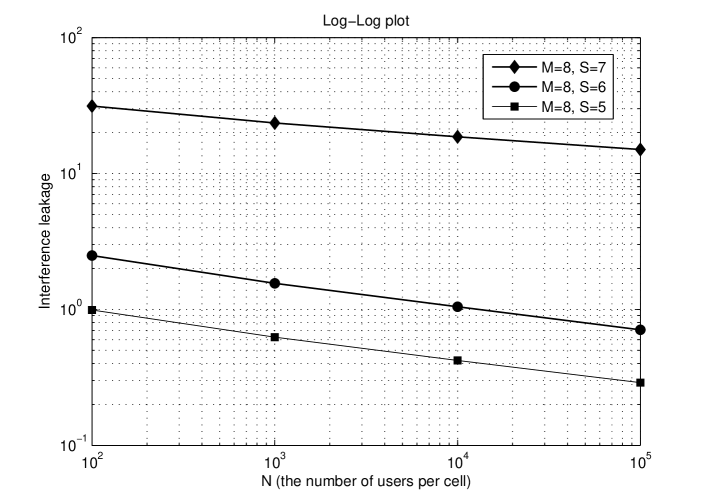
Figure 2: The leakage interference with respect to $N$ for some $S$. The system with $M=8$, $K=2$, and $SK>M$ is considered.

In Fig. 2, The log-log plot of interference leakage versus $N$ is shown as $N$ increases. The interference leakage is interpreted as the total interference power remaining in each desired signal space (from the users in other cells) after the ZF filter is applied, assuming that the received signal power from a desired transmitter is normalized to 1 in the signal space. This performance measure enables us to measure the quality of the proposed OIA scheme, as shown in [9, 30]. We now evaluate the interference leakage for various system parameters. In Fig. 2, the case with $M=8$, $K=2$, and $SK>M$ is considered, where $S$ denotes the number of simultaneously transmitting users per cell. It is shown that when the parameter $S$ varies from 7 to 5, the interference leakage decreases due to less interferers, which is rather obvious. The result, illustrated in Fig. 2, indicates that the interference leakage tends to decrease linearly with $N$, while the slopes of the curves are almost identical to each other as $N$ increases. It is further seen how many users per cell are required to guarantee that the interference leakage is less than an arbitrarily small $\epsilon>0$ for given parameters $M$, $S$, and $K$.

V-B Two-step OIN Protocol

The main result of the paper states that the OIN scheme asymptotically achieves the optimal DoFs in $K$-cell uplink networks. Users are opportunistically selected in the sense of confining the generating interference power to other cell BSs within a constant independent of SNR, while the other opportunistic algorithms aim to obtain the MUD gain by selecting users with the maximum channel gain. We now introduce a two-step opportunistic scheduling method that enables to obtain an additional logarithmic gain, i.e., power gain, similarly as in [17, 18, 19], as well as the full DoF gain.

• Step 1: For the $i$-th cell, $\tilde{M}$ users are first selected according to the user scheduling metric $L_{j}^{i}$ in (3), where $\tilde{M}=\omega(M)$ and $i=1,\cdots,K$. That is, the parameter $\tilde{M}$ needs to scale as a certain function of increasing SNR.

• Step 2: Among the $\tilde{M}$ users, $M$ users with the desired channel gains up to the $M$-th largest one are then chosen based on the metric $\|{\bf h}_{i,\pi_{i}^{\prime}(j)}^{(i)}\|^{2}$, where $\pi_{i}^{\prime}(j)$ denotes the index of users selected in the first step in cell $i$ for $j=\{1,\cdots,\tilde{M}\}$.

From Theorem 1, it is easily shown that if $N=\omega(\mathrm{SNR}^{(K-1)\tilde{M}})$, then the interference in each desired signal space from $\tilde{M}$ selected users per cell is confined within a constant independent of SNR. Hence, similarly as in [19], the received SNR for each symbol would be boosted by $\operatorname{log}\tilde{M}$ whp, compared to that shown in (4), under the condition $\tilde{M}=\omega(M)$. As $\tilde{M}$ scales with SNR (or equivalently $N$), the scaling laws of the sum-rate in (7) can be obtained with respect to $\tilde{M}$, and thus the achievable sum-rate scales as

$$KM\operatorname{log}\left(\text{SNR}\operatorname{log}\tilde{M}\right)$$

whp. Hence, note that the above two-step procedure leads to performance improvement on the sum-rate (but not on the DoFs).

V-C Extension to Multi-carrier Systems

The OIM scheme can easily be applied to multi-carrier systems by executing dimension expansion over the frequency domain. Let $N_{\text{sub}}$ denote the total number of subcarriers, which has no need for tending to infinity. As a single antenna is simply assumed at each BS in the multi-carrier environment, each user transmits a data symbol using $N_{\text{sub}}$ frequency subcarriers and the received signal vector $\mathbf{y}_{i}\in\mathbb{C}^{N_{\text{sub}}\times 1}$ over the frequency domain at BS $i$ can then be expressed as

$$\mathbf{y}_{i}=\sum_{j=1}^{S}\mathbf{H}_{i,j}^{(i)}x_{j}^{(i)}+\sum_{k=1,k\neq i}^{K-1}\sum_{n=1}^{S}\mathbf{H}_{i,n}^{(k)}x_{n}^{(k)}+\mathbf{z}_{i},$$

where $\mathbf{H}_{k,j}^{(i)}\in\mathbb{C}^{N_{\text{sub}}\times 1}$ indicates the frequency response of the channel from the $j$-th user in the $k$-th cell to BS $i$, $\mathbf{z}_{i}\in\mathbb{C}^{N_{\text{sub}}\times 1}$ is the AWGN vector over the frequency domain at BS $i$, and $S\in\{1,\cdots,N_{\text{sub}}\}$ is the number of users transmitting their data simultaneously in each cell. We assume a rich scattering multipath fading environment and thus all elements of $\mathbf{H}_{k,j}^{(i)}$ are assumed to be statistically independent for all $i,k\in\{1,\cdots,K\}$ and $j\in\{1,\cdots,N\}$.

For the OIN and OIA protocols under the multi-carrier model, the user scheduling strategy and its achievability result almost follow the same steps as those shown in Section III. Hence, we mainly focus on the scenario where a beamforming can also be performed at the transmitter side along with the user scheduling.

For example, when the OIA scheme is utilized, it is possible for each user to reduce the amount of interference caused to the BSs in other cells by generating a beamforming matrix and then adjusting its vector directions, while no beamforming is available in Section III since a single transmit antenna is used at each user. The optimal diagonal weight matrix ${\bf W}_{j}^{(i)}\in\mathbb{C}^{N_{\text{sub}}\times N_{\text{sub}}}$ can be designed at each user in the sense of minimizing the total sum of $K-1$ LIF values defined in (5), i.e., the metric $L_{j}^{i}$:

$${\bf W}_{j}^{(i)}=\operatorname{arg}\operatornamewithlimits{min}_{{\bf W}\in\mathbb{C}^{N_{\text{sub}}\times N_{\text{sub}}}}\sum_{l=1,k\neq i}^{K}\left\|\text{Proj}_{U^{(l)}}\left({\bf W}\mathbf{H}_{l,j}^{(i)}\right)\right\|^{2}$$ (16)

$$\textrm{subject to}\quad\|\text{diag}({\bf W})\|^{2}=1,$$

where $U^{(l)}$ denotes the null space of the interference subspace in the $l$-th cell. Note that each user does not need to feed back its optimal weight matrix in (16) to its home cell BS. Let ${\bf W}_{j,\text{opt}}^{(i)}$ denote the optimal solution of (16). The $j$-th user in the $i$-th cell then feeds back the following scheduling metric $\widetilde{L}_{j}^{i}$ that can be computed again by applying the optimal weight matrix:

$$\widetilde{L}_{j}^{i}=\sum_{l=1,k\neq i}^{K}\left\|\text{Proj}_{U^{(l)}}\left(\mathbf{\tilde{H}}_{l,j}^{(i)}\right)\right\|^{2},$$ (17)

where

$$\mathbf{\tilde{H}}_{l,j}^{(i)}={\bf W}_{j,\text{opt}}^{(i)}\mathbf{H}_{l,j}^{(i)}.$$

Thereafter, BS $i$ selects a set of $S$ users who feed back the values up to the $S$-th smallest one in (17) among all users in a cell, where $S\in\{1,\cdots,N_{\text{sub}}-1\}$. This per-user optimization procedure may yield less amount of the LIF at each BS than that of the conventional approach without beamforming. In other words, by applying the beamforming design as well as the user scheduling, the minimum required number $N$ of users per cell such that a given LIF value is guaranteed may scale slower than $\text{SNR}^{(K-1)S}$ shown in Theorem 1, thus leading to more feasible network realization.

V-D Comparison with the Existing Methods

In this subsection, the proposed scheme is compared with the two existing strategies [13, 14] that also achieve the optimal DoFs in $K$-cell uplink networks. We now focus on the case for $M=1$, i.e., $K$-cell IMAC model with a single antenna at each BS, as in [13, 14]. Under the model, all of the OIN and two existing IA methods achieve $K$ DoFs asymptotically as the number $N$ of users in a cell tends to infinity, while their channel models and (analytical) approaches are quite different from each other.

Since the two schemes [13, 14] are analyzed in a deterministic manner, it is possible to achieve a non-zero number of DoFs, less than $K$, even for finite $N$ (independent of SNR). In contrast, the achievability result of the OIN scheme is shown based on a probabilistic approach, where infinitely many number of users per cell, which scales faster than $\text{SNR}^{K-1}$, is needed to guarantee full DoFs without any dimension expansion.

Now let us turn to discussing channel modelings. The subspace-based IA scheme [13] was introduced in $K$-cell uplink networks allowing dimension expansion over the frequency domain, where it requires $(K-1)$-level decomposability of channels at each link since designing transmit vectors shown in [13] takes advantage of decomposed channel matrices. Accordingly, single-path random delay channels are preferable due to the fact that they are $(K-1)$-level decomposable and thus are convenient to align interfering signals in practice. If we assume multipath frequency selective channels, then the whole channel band should be splitted into multiple sub-bands, each of which needs to be within coherence bandwidth and to occupy many subcarriers for dimension expansion, thereby yielding practical challenges. On the other hand, our scheme works well with rich scattering environments, because it exploits channel randomness for either nulling or aligning interfering signals. However, a highly correlated channel among users (e.g., relatively poor scattering environment) may result in performance degradation for the proposed scheme, since it is difficult to select users such that the sum of LIF values is small enough. In [14], another IA scheme, named as real IA, has been introduced in cellular uplink networks with time-invariant real channel coefficients—the IA operation is conducted in signal scale but not in signal vector space. Specifically, the strategy exploits the fact that a real line consists of infinite rational dimensions. Instead, under the complex channel environment, a multi-dimensional Euclidean space is taken into account to align interference in signal vector space, as shown in the conventional IA methods [7, 8, 10, 11, 12, 13].

VI Conclusion

Two types of OIM protocols were proposed in wireless $K$-cell uplink networks, where they do not require the global CSI, infinite dimension extension, and parameter adjustment through iteration. The achievable DoFs were then analyzed—the OIM protocol asymptotically achieves $KS$ DoFs as long as $N$ scales faster than $\text{SNR}^{(K-1)S}$, where $S\in\{1,\cdots,M\}$. It has been seen that there exists a trade-off between the achievable DoFs and the parameter $N$ based on the two OIM schemes. From the result of the upper bound on the DoFs, it was shown that the OIM protocol with $S=M$ achieves the optimal DoFs with the help of the MUD gain. In addition, the two-step scheduling method that can further obtain a power gain has been shown, and extension to the multi-carrier systems has been discussed.

Appendix A Appendix

A-A Proof of Lemma 1

The cdf $F_{L}(l)$ of the metric $L_{j}^{i}$ satisfies the inequality $\gamma(z,x)\geq\frac{1}{z}x^{z}e^{-1}$ for $z>0$ and $0\leq x<1$ since

$$\gamma(z,x) =\frac{1}{z}x^{z}e^{-x}+\frac{1}{z}\gamma(z+1,x)$$

$$=\frac{1}{z}x^{z}e^{-x}+\frac{1}{z(z+1)}x^{{z+1}}e^{-x}+\cdots$$

$$\geq\frac{1}{z}x^{z}e^{-1}.$$

Similarly, $\gamma(z,x)$ is upper-bounded by $2z^{-1}x^{z}$ for $z>0$ and $0\leq x<1$ from the fact that

$$\gamma(z,x) =\frac{1}{z}x^{z}e^{-x}+\frac{1}{z}\gamma(z+1,x)$$

$$\leq\frac{1}{z}x^{z}e^{-x}+\frac{1}{z}x^{z}e^{-x}\sum_{i=1}^{\infty}\left(\frac{x}{z+1}\right)^{i}$$

$$=\left(\frac{1}{z}+\frac{x}{z+1-x}\right)x^{z}e^{-x}$$

$$\leq\frac{2}{z}x^{z}.$$

Applying the above bounds to (9), we finally obtain (10), which completes the proof.

A-B Proof of Theorem 2

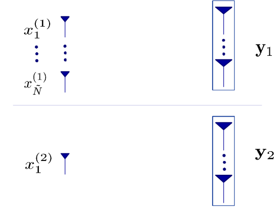
Figure 3: The two-cell IMAC model defined in Section IV.

Although the proof technique is essentially similar to that of [8, 35], the whole steps are shown here for completeness. Let $W_{j}^{(i)}$ and $R_{j}^{(i)}$ denote the message and its transmission rate of user $j$ in the $i$-th cell, respectively. Consider a certain two-cell IMAC model illustrated in Fig. 3, where we eliminate messages $W_{j}^{(3)},W_{j}^{(4)},\cdots,W_{j}^{(K)}$ for all $j\in\{1,\cdots,\tilde{N}\}$ as well as $W_{j}^{(2)}$ for $j\in\{2,\cdots,\tilde{N}\}$. We then obtain the following two equations:

$$\mathbf{y}_{1} = \sum_{j=1}^{\tilde{N}}\mathbf{h}_{1,j}^{(1)}x_{j}^{(1)}+\mathbf{h}_{1,1}^{(2)}x_{1}^{(2)}+\mathbf{z}_{1}$$

and

$$\mathbf{y}_{2} = \sum_{j=1}^{\tilde{N}}\mathbf{h}_{2,j}^{(1)}x_{j}^{(1)}+\mathbf{h}_{2,1}^{(2)}x_{1}^{(2)}+\mathbf{z}_{2},$$ (18)

which yield

$$\mathbf{y}_{2}^{\prime} = \mathbf{h}_{1,1}^{(2)}\left(\mathbf{h}_{2,1}^{(2)\dagger}\mathbf{h}_{2,1}^{(2)}\right)^{-1}\mathbf{h}_{2,1}^{(2)\dagger}\sum_{j=1}^{\tilde{N}}\mathbf{h}_{2,j}^{(1)}x_{j}^{(1)}+\mathbf{h}_{1,1}^{(2)}x_{1}^{(2)}+\mathbf{z}_{2}^{\prime}$$

after multiplying some channel matrices at both sides of (18), where

$$\mathbf{z}_{2}^{\prime}\sim\mathcal{CN}\left(\mathbf{0},N_{0}\left(\mathbf{h}_{1,1}^{(2)}\left(\mathbf{h}_{2,1}^{(2)\dagger}\mathbf{h}_{2,1}^{(2)}\right)^{-1}\mathbf{h}_{2,1}^{(2)\dagger}\right)\left(\mathbf{h}_{1,1}^{(2)}\left(\mathbf{h}_{2,1}^{(2)\dagger}\mathbf{h}_{2,1}^{(2)}\right)^{-1}\mathbf{h}_{2,1}^{(2)\dagger}\right)^{\dagger}\right).$$

Suppose that $\mathbf{z}_{1}=\bar{\mathbf{z}}+\bar{\mathbf{z}}_{1}$ and $\mathbf{z}_{2}^{\prime}=\bar{\mathbf{z}}+\bar{\mathbf{z}}_{2}$, where

$$\bar{\mathbf{z}}\sim\mathcal{CN}\left(\mathbf{0},\alpha N_{0}\mathbf{I}_{M}\right),$$

$$\bar{\mathbf{z}}_{1}\sim\mathcal{CN}\left(\mathbf{0},(1-\alpha)N_{0}\mathbf{I}_{M}\right),$$

and

$$\bar{\mathbf{z}}_{2}\sim\mathcal{CN}\left(\mathbf{0},N_{0}\left(\mathbf{h}_{1,1}^{(2)}\left(\mathbf{h}_{2,1}^{(2)\dagger}\mathbf{h}_{2,1}^{(2)}\right)^{-1}\mathbf{h}_{2,1}^{(2)\dagger}\right)\left(\mathbf{h}_{1,1}^{(2)}\left(\mathbf{h}_{2,1}^{(2)\dagger}\mathbf{h}_{2,1}^{(2)}\right)^{-1}\mathbf{h}_{2,1}^{(2)\dagger}\right)^{\dagger}-\alpha N_{0}\mathbf{I}_{M}\right).$$

Here, $\alpha$ is given by

$$\alpha=\operatornamewithlimits{min}\left(1,\lambda_{\operatornamewithlimits{min}}\left(\left(\mathbf{h}_{1,1}^{(2)}\left(\mathbf{h}_{2,1}^{(2)\dagger}\mathbf{h}_{2,1}^{(2)}\right)^{-1}\mathbf{h}_{2,1}^{(2)\dagger}\right)\left(\mathbf{h}_{1,1}^{(2)}\left(\mathbf{h}_{2,1}^{(2)\dagger}\mathbf{h}_{2,1}^{(2)}\right)^{-1}\mathbf{h}_{2,1}^{(2)\dagger}\right)^{\dagger}\right)\right).$$

Then by using Fano’s inequality [36], we have

$$\sum_{j=1}^{\tilde{N}}R_{j}^{(1)}+R_{1}^{(2)}\!\!\!\!\!\!\! \leq I\left(W_{1}^{(1)},\cdots,W_{\tilde{N}}^{(1)};\mathbf{y}_{1}\right)+I\left(W_{1}^{(2)};\mathbf{y}_{2}\right)+\epsilon_{0}$$ (19)

$$=I\left(W_{1}^{(1)},\cdots,W_{\tilde{N}}^{(1)};\mathbf{y}_{1}\right)+I\left(W_{1}^{(2)};\mathbf{y}_{2}^{\prime}\right)+\epsilon_{0}$$

$$\leq I\left(W_{1}^{(1)},\cdots,W_{\tilde{N}}^{(1)};\mathbf{y}_{1}\right)$$

$$\quad+I\biggl{(}W_{1}^{(2)};\mathbf{h}_{1,1}^{(2)}\left(\mathbf{h}_{2,1}^{(2)\dagger}\mathbf{h}_{2,1}^{(2)}\right)^{-1}\mathbf{h}_{2,1}^{(2)\dagger}\sum_{j=1}^{\tilde{N}}\mathbf{h}_{2,j}^{(1)}x_{j}^{(1)}+\mathbf{h}_{1,1}^{(2)}x_{1}^{(2)}+\bar{\mathbf{z}}$$

$$\quad\bigg{|}W_{1}^{(1)},\cdots,W_{\tilde{N}}^{(1)},x_{1}^{(1)},\cdots,x_{\tilde{N}}^{(1)}\biggr{)}+\epsilon_{0}$$

$$=I\left(W_{1}^{(1)},\cdots,W_{\tilde{N}}^{(1)};\mathbf{y}_{1}\right)$$

$$\quad+I\biggl{(}W_{1}^{(2)};\mathbf{h}_{1,1}^{(2)}x_{1}^{(2)}+\bar{\mathbf{z}}\left|W_{1}^{(1)},\cdots,W_{\tilde{N}}^{(1)},x_{1}^{(1)},\cdots,x_{\tilde{N}}^{(1)}\right)+\epsilon_{0}$$

$$\leq I\left(W_{1}^{(1)},\cdots,W_{\tilde{N}}^{(1)};\sum_{j=1}^{\tilde{N}}\mathbf{h}_{1,j}^{(1)}x_{j}^{(1)}+\mathbf{h}_{1,1}^{(2)}x_{1}^{(2)}+\bar{\mathbf{z}}\right)$$

$$\quad+I\biggl{(}W_{1}^{(2)};\sum_{j=1}^{\tilde{N}}\mathbf{h}_{1,j}^{(1)}x_{j}^{(1)}+\mathbf{h}_{1,1}^{(2)}x_{1}^{(2)}+\bar{\mathbf{z}}$$

$$\quad\bigg{|}W_{1}^{(1)},\cdots,W_{\tilde{N}}^{(1)},x_{1}^{(1)},\cdots,x_{\tilde{N}}^{(1)}\biggr{)}+\epsilon_{0}$$

$$=I\left(W_{1}^{(1)},\cdots,W_{\tilde{N}}^{(1)},W_{1}^{(2)};\sum_{j=1}^{\tilde{N}}\mathbf{h}_{1,j}^{(1)}x_{j}^{(1)}+\mathbf{h}_{1,1}^{(2)}x_{1}^{(2)}+\bar{\mathbf{z}}\right)+\epsilon_{0}$$

for an arbitrarily small $\epsilon_{0}>0$, where the second and third inequalities come from reducing noise variance. The right-hand-side of (19) represents the sum capacity of a MAC with an $M$ antenna receiver and $\tilde{N}$ single-antenna transmitters, and thus if $\tilde{N}\geq M$, then the number of DoFs for the MAC is given by $M$ [34, 37]. Hence, simply assuming $\tilde{N}=N$, we obtain the following upper bounds:

$$\sum_{j=1}^{N}R_{j}^{(1)}+R_{1}^{(2)}\leq M\operatorname{log}\text{SNR}+o\left(\operatorname{log}\text{SNR}\right)$$

and

$$\sum_{j=1}^{N}d_{j}^{(1)}+d_{1}^{(2)}\leq M.$$

Similarly, for any $k\in\{1,2,\cdots,N\}$, we obtain

$$\sum_{j=1}^{N}d_{j}^{(1)}+d_{k}^{(2)}\leq M$$ (20)

and

$$d_{k}^{(1)}+\sum_{j=1}^{N}d_{j}^{(2)}\leq M.$$ (21)

Adding up all the possible combinations over $k$ shown in (20) and (21), we finally have

$$\sum_{j=1}^{N}d_{j}^{(i)}\leq\frac{NM}{N+1}$$

at a given cell $i$. Since there are $K$ cells in the IMAC model, the total number of DoFs is upper-bounded by (15), which completes the proof.

Acknowledgement

The authors would like to thank Sae-Young Chung for his helpful discussions.

References

- [1] A. D. Wyner, “Shannon-theoretic approach to a Gaussian cellular multiple-access channel,” IEEE Trans. Inf. Theory, vol. 40, no. 6, pp. 1713–1727, Nov. 1994.
- [2] S. Shamai (Shitz) and A. D. Wyner, “On information theoretic considerations for symmetric cellular multiple access communication channels–Part I,” IEEE Trans. Inf. Theory, vol. 43, no. 6, pp. 1877–1894, Nov. 1997.
- [3] S. Shamai (Shitz) and A. D. Wyner, “On information theoretic considerations for symmetric cellular multiple access communication channels–Part II,” IEEE Trans. Inf. Theory, vol. 43, no. 6, pp. 1895–1911, Nov. 1997.
- [4] O. Somekh and S. Shamai (Shitz), “Shannon-theoretic approach to a Gaussian cellular multi-access channel with fading,” IEEE Trans. Inf. Theory, vol. 46, no. 4, pp. 1401–1425, Jul. 2000.
- [5] O. Somekh, B. M. Zaidel, and S. Shamai (Shitz), “Sum rate characterization of joint multiple cell-site processing,” IEEE Trans. Inf. Theory, vol. 53, no. 12, pp. 4473–4497, Dec. 2007.
- [6] N. Levy and S. Shamai (Shitz), “Information theoretic aspects of users’ activity in a Wyner-like cellular model,” IEEE Trans. Inf. Theory, vol. 56, no. 5, pp. 2241–2248, May 2010.
- [7] M. A. Maddah-Ali, A. S. Motahari, and A. K. Khandani, “Communication over MIMO X channels: interference alignment, decomposition, and performance analysis,” IEEE Trans. Inf. Theory, vol. 54, no. 8, pp. 3457–3470, Aug. 2008.
- [8] V. R. Cadambe and S. A. Jafar, “Interference alignment and degrees of freedom of the -user interference channel,” IEEE Trans. Inf. Theory, vol. 54, no. 8, pp. 3425–3441, Aug. 2008.
- [9] K. Gomadam, V. R. Cadambe, and S. A. Jafar, “Approaching the capacity of wireless networks through distributed interference alignment,” preprint, [Online]. Available: http://arxiv.org/abs/0803.3816.
- [10] T. Gou and S. A. Jafar, “Degrees of freedom of the -user MIMO interference channel,” preprint, [Online]. Available: http://arxiv.org/abs/0809.0099.
- [11] V. R. Cadambe and S. A. Jafar, “Degrees of freedom of wireless networks,” preprint, [Online]. Available: http://arxiv.org/abs/0711.2824.
- [12] S. A. Jafar and S. Shamai (Shitz), “Degrees of freedom region of the MIMO X channel,” IEEE Trans. Inf. Theory, vol. 54, no. 1, pp. 151–170, Jan. 2008.
- [13] C. Suh and D. Tse, “Interference alignment for celluar networks,” in Proc. 46th Annual Allerton Conf. on Commun., Control, and Computing, Monticello, IL, Sep. 2008.
- [14] A. S. Motahari, O. Gharan, M.-A. Maddah-Ali, and A. K. Khandani, “Real interference alignment: exploiting the potential of single antenna systems,” IEEE Trans. Inf. Theory, submitted for publication, [Online]. Available: http://arxiv.org/abs/0908.2282.
- [15] N. Lee, W. Shin, and B. Clerckx, “Interference alignment with limited feedback on two-cell interfering two-user MIMO-MAC,” preprint, [Online]. Available: http://arxiv.org/abs/1010.0933.
- [16] B. Nazer, M. Gastpar, S. A. Jafar, and P. Viswanath , “Ergodic interference alignment,” in Proc. IEEE Int. Symp. Inf. Theory (ISIT), Seoul, Korea, Jun.-Jul. 2009, pp. 1769–1773.
- [17] R. Knopp and P. Humblet, “Information capacity and power control in single cell multiuser communications,” in Proc. IEEE Int. Conf. Commun. (ICC), Seattle, WA, Jun. 1995, pp. 331–335.
- [18] P. Viswanath, D. N. C. Tse, and R. Laroia, “Opportunistic beamforming using dumb antennas,” IEEE Trans. Inf. Theory, vol. 48, no. 6, pp. 1277–1294, Aug. 2002.
- [19] M. Sharif and B. Hassibi, “On the capacity of MIMO broadcast channels with partial side information,” IEEE Trans. Inf. Theory, vol. 51, no. 2, pp. 506–522, Feb. 2005.
- [20] Z. Wang, M. Ji, H. R. Sadjadpour, and J. J. Garcia-Luna-Aceves, “Interference management: a new paradigm for wireless cellular networks,” in Proc. IEEE Military Commun. Conf. (MILCOM), Boston, MA, Oct. 2009, pp. 1–6.
- [21] L. Dritsoula, Z. Wang, H. R. Sadjadpour, and J. J. Garcia-Luna-Aceves, “Antenna selection for opportunistic interference management in MIMO broadcast channels,” in Proc. IEEE Signal Process. Advances Wireless Commun. (SPAWC), Marrakech, Morocco, Jun. 2010, pp. 1–5.
- [22] S. Cui, A. M. Haimovich, O. Somekh, and H. V. Poor, “Opportunistic relaying in wireless networks,” IEEE Trans. Inf. Theory, vol. 55, no. 11, pp. 5121–5137, Nov. 2009.
- [23] W.-Y. Shin, S.-Y. Chung, and Y. H. Lee, “Improved power–delay trade-off in wireless networks using opportunistic routing,” IEEE Trans. Inf. Theory, under revision for possible publication, [Online]. Available: http://arxiv.org/abs/0907.2455.
- [24] T. W. Ban, W. Choi, B. C. Jung, and D. K. Sung, “Multi-user diversity in a spectrum sharing system,” IEEE Trans. Wireless Commun., vol. 8, no. 1, pp. 102–106, Jan. 2009.
- [25] C. Shen and M. P. Fitz, “Opportunistic spatial orthogonalization and its application to fading cognitive radio networks,” preprint, [Online]. Available: http://arxiv.org/abs/0904.4283.
- [26] S.-W. Jeon and S.-Y. Chung, “Capacity of a class of a multi-source relay networks,” IEEE Trans. Inf. Theory, under revision for possible publication, [Online], Available: http://arxiv.org/abs/0907.2510.
- [27] S. M. Perlaza, M. Debbah, S. Lasaulce, and J. -M. Chaufray, “Opportunistic interference alignment in MIMO interference channels,” in Proc. IEEE Personal, Indoor and Mobile Radio Commun. Symp. (PIMRC), Cannes, France, Sep. 2008, pp. 1–5.
- [28] S. M. Perlaza, N. Fawaz, S. Lasaulce, and M. Debbah, “From spectrum pooling to space pooling: opportunistic interference alignment in MIMO cognitive networks,” IEEE Trans. Signal Process., vol. 58, no. 7, pp. 3728–3741, Jul. 2010.
- [29] R. Zhang and Y. C. Liang, “Exploiting multi-antennas for opportunistic spectrum sharing in cognitive radio networks,” IEEE J. Select. Topics Signal Process., submitted for publication, [Online]. Available: http://arxiv.org/abs/0711.4414.
- [30] H. Yu and Y. Sung, “Least squares approach to joint beam design for interference alignment in multiuser multi-input multi-output interference channels,” IEEE Trans. Signal Process., vol. 58, no. 9, pp. 4960–4966, Sep. 2010.
- [31] T. Tang, R. W. Heath, Jr., S. Cho, and S. Yun, “Opportunistic feedback in multiuser MIMO systems with linear receivers,” IEEE Trans. Commun., vol. 55, no. 5, pp. 1020–1032, May 2007.
- [32] L. Zheng and D. N. C. Tse, “Diversity and multiplexing: a fundamental tradeoff in multiple-antenna channels,” IEEE Trans. Inf. Theory, vol. 49, no. 5, pp. 1073–1096, May 2003.
- [33] D. E. Knuth, “Big Omicron and big Omega and big Theta,” ACM SIGACT News, vol. 8, pp. 18–24, Apr.-Jun. 1976.
- [34] D. Tse and P. Viswanath, Fundamentals of Wireless Communication, New York: Cambridge University Press, 2005.
- [35] S. A. Jafar and M. J. Fakhereddin, “Degrees of freedom for the MIMO interference chanel,” IEEE Trans. Inf. Theory, vol. 53, no. 7, pp. 2637–2642, Jul. 2007.
- [36] T. M. Cover and J. A. Thomas, Elements of Information Theory, New York: Wiley, 1991.
- [37] P. Viswanath and D. N. C. Tse, “Sum capacity of the vector Gaussian broadcast channel and uplink-downlink duality,” IEEE Trans. Inf. Theory, vol. 49, no. 8, pp. 1912–1921, Aug. 2003.