Finite-size effects on the radiative energy loss of a fast parton in hot and dense strongly interacting matter

Abstract

We consider finite-size effects on the radiative energy loss of a fast parton moving in a finite temperature strongly interacting medium, using the light cone path integral formalism put forward by Zakharov. We present a convenient reformulation of the problem which makes possible its exact numerical analysis. This is done by introducing the concept of a radiation rate in the presence of finite-size effects. This effectively extends the finite-temperature approach of AMY (Arnold, Moore, and Yaffe) to include interference between vacuum and medium radiation. We compare results with those obtained in the regime considered by AMY, with those obtained at leading order in an opacity expansion, and with those obtained deep in the LPM (Landau-Pomeranchuk-Migdal) regime.

I Introduction

The physics of strongly interacting matter in extreme conditions of temperature and density continues to be one of the most active and fascinating fields of contemporary subatomic physics. It straddles nuclear and particle physics, and enjoys an immediate connection with the science of dense stellar objects. The liveliness of this discipline owes in no small part to the vibrant experimental programs and active theoretical support that characterize it. In this context, it is fair to write that the Relativistic Heavy Ion Collider (RHIC) continues to be a center of activity, and that this facility now boasts several compelling results white . For example, the measurement of a strong suppression of hard partons in nucleus-nucleus collisions has been spectacular RAA , confirming - and even exceeding - early expectations gyuwang . In addition, the empirical success of the hydrodynamical modelling of soft hadronic observables has been an important factor in popularizing the concept of a strongly coupled quark-gluon plasma (sQGP) sqgp .

The experimental measurements of the quenching of hard QCD jets have stimulated the theory community and several approaches based on perturbative QCD (pQCD) have been put forward to explain them. The formalisms differ in the details by which they treat the QCD medium, but all include the coherence built in multiple scatterings: The so-called Landau-Pomeranchuk-Migdal (LPM) effect LPM . Recently, some work has been devoted to comparing the different theoretical approaches, to highlight the similarities, and to point out the differences TECHQM . Importantly, the medium in a relativistic heavy ion collision is a dynamical one: It rapidly evolves with time. It is therefore important to separate the consequences of the dynamical evolution scenario from those related to basic and fundamental differences in the theory bass . In order to highlight as clearly as possible the different assumptions and ingredients going into the different theory approaches, it has been useful to imagine an idealized setting where the basic formalisms can simply be compared without the complications of realistic dynamics: The “QCD brick”. The brick is a slab of strongly interacting partonic matter, in thermal equilibrium at a temperature $T$. The goal then consists of analyzing the energy loss of a fast parton, propagating in, and interacting with, the medium. With this philosophy in mind, we concentrate in this paper on AMY, a formalism which stems from finite-temperature field theory and treats the QCD medium dynamically. Its basic premises were established in a series of papers written in the last decade AMY ; JeonMoore , and some of its phenomenological consequences have also been investigated bass ; Qin:2009bk ; AMYpheno . The original formulation of AMY was in momentum space, and effects owing to the finite size of the emitting region were therefore a challenge to include. This paper follows the techniques of the light-cone path integral formalism elaborated by Zakharov ZakharovL ; ZakharovBulk and which is known to lead to results similar to those of Baier-Dokshitzer-Mueller-Peigne-Schiff (BDMPS) BDMPS and incorporate these effects into the AMY description. The effects of a finite formation time on inelastic radiation rates and on the time-dependent parton momentum distributions are explored, in order to eventually assess the consequences of this additional consideration on the phenomenology of RHIC and on that of the LHC.

Our paper is organized as follows: In the next section, the basic theoretical building blocks of our approach are laid down. In what regards radiation rates, we show that in well-defined limits our results coincide with those obtained in other treatments. Next we explore numerically the effect of the finite formation time on radiation rates, and then on the parton distribution functions. We explore the dynamics of the radiated gluons, and then summarize and conclude.

II Formalism

II.1 Starting point

The starting point here will be Eq. (4) of Ref. ZakharovBulk expressing the total probability for parton $a$, produced at time $t=0$ with energy $p$, to emit a pair $b,c$ of bremsstrahlung partons with energies $k$, $p{-}k$:

$$\frac{dP^{a}_{bc}}{dk}=\frac{P^{a(0)}_{bc}(x)}{\pi p}\times{\rm Re}\,\int_{0}^{\infty}dt_{1}\int_{t_{1}}^{\infty}dt_{2}\frac{\partial}{\partial{\bf x}}{\cdot}\frac{\partial}{\partial{\bf y}}\left[K(t_{2},{\bf x};t_{1},{\bf y})-\mbox{(vac)}\right]_{{\bf x}={\bf y}=0}.$$ (1)

For the benefit of the reader, this equation will be re-derived in the next section. In Eq. (1), $K(t_{2},{\bf x};t_{1},{\bf y})$ is $[p/(2k(p{-}k))]^{2}$ times the propagator associated with the light-cone Hamiltonian

$$H = \delta E({\bf p})-i\mathcal{C}_{3},$$ (2a)

$$\delta E({\bf p}) \equiv \frac{p{\bf p}^{2}}{2k(p{-}k)}+\frac{m_{b}^{2}}{2k}+\frac{m_{c}^{2}}{2(p{-}k)}-\frac{m_{a}^{2}}{2p},$$ (2b)

$$\mathcal{C}_{3}({\bf x}) \equiv \frac{C_{b}{+}C_{c}{-}C_{a}}{2}v_{2}({\bf x})+\frac{C_{a}{+}C_{c}{-}C_{b}}{2}v_{2}(\frac{k}{p}{\bf x})+\frac{C_{a}{+}C_{b}{-}C_{c}}{2}v_{2}(\frac{p{-}k}{p}{\bf x}),$$ (2c)

which acts on wave-function $\psi({\bf x})$ on the transverse plane; $m_{a,b,c}$ and $C_{a,b,c}$ are the respective masses (including thermal corrections) and group theory Casimirs of the particles involved ($C_{A}=3$ for gluons and $C_{F}=\frac{4}{3}$ for quarks in QCD); $C_{\textrm{F}}v_{2}({\bf x})$ is the dipole propagation amplitude per unit length for a $q\overline{q}$ pair. $P^{a(0)}_{bc}(x)$ are the DGLAP splitting kernels DGLAP for the process $a\to bc$, with $x=\frac{k}{p}$ the longitudinal momentum fraction of particle $b$:

$$P^{a(0)}_{bc}(x)=\left\{\begin{array}[]{ll}g^{2}C_{\textrm{F}}\frac{1+(1{-}x)^{2}}{x},&q\to gq\\ g^{2}C_{A}\frac{1{+}x^{4}{+}(1{-}x)^{4}}{x(1{-}x)},&g\to gg\\ 2g^{2}N_{\textrm{F}}T_{\textrm{F}}\left[x^{2}+(1{-}x)^{2}\right],&g\to q\overline{q}\\ e^{2}\frac{1+(1{-}x)^{2}}{x}&e\to\gamma e\end{array}\right.$$ (3)

Final states $bc$ and $cb$ are equivalent and should be counted only once. In particular, only the region $x<\frac{1}{2}$ is to be included in $g\to gg$. For QCD, $C_{\textrm{F}}=\frac{4}{3}$, $C_{\textrm{A}}=3$ and $N_{\textrm{F}}T_{\textrm{F}}=\frac{3}{2}$.

At this stage, it is appropriate to observe that the formula contains two time integrations, which, ultimately, correspond to two emission vertices – one in the matrix element and one in its complex conjugate. Since no emission occurs before the jet is produced, both integrations begin at $t=0$. But since the radiation can be emitted at any time afterwards, they extend to infinity. Hence (1) contains two non-compact time integrations, which, in general, have to be performed numerically.

II.2 Re-organization

We re-arrange Eq. (1) in two steps in order to make it more suitable for our analysis. Mainly, we wish to remove the non-compact time integrations. First, we Fourier-transform it to transverse momentum space, with $\int_{\bf k}\equiv\int\frac{d^{2}{\bf k}}{(2\pi)^{2}}$,

$$\frac{dP^{a}_{bc}}{dk}=\frac{P^{a(0)}_{bc}(x)}{\pi p}\times{\rm Re}\,\int_{0}^{\infty}dt_{1}\int_{t_{1}}^{\infty}dt_{2}\int_{{\bf q},{\bf p}}{\bf q}{\cdot}{\bf p}\left[K(t_{2},{\bf q};t_{1},{\bf p})-\mbox{(vac)}\right].$$

In Fourier space, $\mathcal{C}_{3}$ becomes the Boltzmann-like collision operator

$$\mathcal{C}\,\psi({\bf p}) = \int_{\bf q}C({\bf q})\left\{\frac{C_{b}{+}C_{c}{-}C_{a}}{2}[\psi({\bf p})-\psi({\bf p}{-}{\bf q})]\right.$$ (4)

$$\left.\hskip 48.36958pt+\frac{C_{a}{+}C_{c}{-}C_{b}}{2}[\psi({\bf p})-\psi({\bf p}{+}\frac{k}{p}{\bf q})]\right.$$

$$\left.\hskip 48.36958pt+\frac{C_{a}{+}C_{b}{-}C_{c}}{2}[\psi({\bf p})-\psi({\bf p}{+}\frac{p{-}k}{p}{\bf q})]\right\}\ ,$$

and $C({\bf q})$ is related to the dipole amplitude via $v_{2}({\bf x})\equiv\int_{\bf q}C({\bf q})\left(1-e^{i{\bf q}{\cdot}{\bf x}}\right)$. This function can also be described as the Casimir-stripped elastic collision rate for a hard particle:

$$C({\bf q})=\frac{1}{C_{\textrm{s}}}(2\pi)^{2}\frac{d^{2}\Gamma_{\textrm{el}}({\bf q})}{d^{2}{\bf q}}.$$

No confusion should arise between the function $C({\bf q})$ and the Casimirs $C_{s}$.

The second step is to make the time integrations compact. At large times, there are no collisions and $K$ depends on time only through phases, which can be integrated exactly. We use this when integrating by parts:

$$\int_{t_{1}}^{\infty}dt_{2}K(t_{2},{\bf q};t_{1},{\bf p}) \equiv \int_{t_{1}}^{\infty}dt_{2}\,\left[\frac{d}{dt_{2}}\left(\frac{e^{-i\delta E({\bf q})t_{2}}}{-i\delta E({\bf q})}\right)\right]e^{i\delta E({\bf q})t_{2}}K(t_{2},{\bf q};t_{1},{\bf p})$$ (5)

$$= \frac{1}{-i\delta E({\bf q})}K(\infty,{\bf q};t_{1},{\bf p})-\frac{1}{-i\delta E({\bf q})}K(t_{1},{\bf q};t_{1},{\bf p})$$

$$+\int_{t_{1}}^{\infty}dt\frac{i}{\delta E({\bf q})}\mathcal{C}(t)K(t,{\bf q};t_{1},{\bf p}).$$

The first, rapidly oscillating, term on the second line disappears, owing to the conventional convergence factor $e^{-\epsilon t}$ implicit in Eq. (1). The second term is closely related to the vacuum (DGLAP) radiation, and for the moment we simply cancel it against the vacuum subtraction. In fact, this cancellation is not exact and a remainder associated with the thermal masses will remain; we postpone its discussion to section IV. For now, only the last term survives, giving

$$\frac{dP^{a}_{bc}}{dk}=\frac{P^{a(0)}_{bc}(x)}{\pi p}\times{\rm Re}\,\int_{0}^{\infty}dt\int_{0}^{t}dt_{1}\int_{{\bf q},{\bf p}}\frac{i{\bf q}{\cdot}{\bf p}}{\delta E({\bf q})}\mathcal{C}(t)K(t,{\bf q};t_{1},{\bf p}).$$

In this form, it is natural to take a derivative with respect to $t$ to define a radiation rate:

$$\frac{d\Gamma^{a}_{bc}(t)}{dk}\equiv\frac{P^{a(0)}_{bc}(x)}{\pi p}\times{\rm Re}\,\int_{0}^{t}dt_{1}\int_{{\bf q},{\bf p}}\frac{i{\bf q}{\cdot}{\bf p}}{\delta E({\bf q})}\mathcal{C}(t)K(t,{\bf q};t_{1},{\bf p}).$$ (6)

This is the formula which we shall study in this paper. It defines a radiation rate in terms of a single, compact, time integration that may conveniently be computed numerically. By construction, its content is fully equivalent to that in the BDMPS-Z probability, Eq. (1); its time integral reproduces the latter. Details of its numerical implementation are given in Appendix A.

It is important to mention that a radiation rate is never uniquely defined. Indeed, the emission time of a given quanta is itself ambiguous up to a so-called formation time. Different prescriptions may lead to different time-dependent rates all associated with the same time-integrated probability. The present prescription is to locate the emission at the time $t$, which corresponds physically to the time of the last collision that influences the emission. This is a reasonable choice, as it is located between the two emission vertices. It is also a particularly natural and convenient choice because it causes the medium-induced radiation to stop outside the medium, that is, $\Gamma$ is zero when $\mathcal{C}$ vanishes. In particular, for the brick problem, $\Gamma$ is zero after exiting the brick. Nevertheless, all possible interference effects (including LPM interference), and memory effects, are included through the non-local kernel $K$.

III Physical interpretation of the formula

We now provide a heuristic derivation of our formula (6), as promised. This will help highlight its underlying assumptions and regime of validity. In this section we also discuss various analytical limits which are related to approximations used in the literature.

III.1 Heuristic derivation of Eq. (1)

Numerous derivations of formulae similar to (1) exist, exploiting one formalism or another BDMPS ; ZakharovL ; GLV0 ; AMY ; aurzak . We believe that the assumptions to be presented here, which did not previously appear with such generality, suffice for its validity.

The four assumptions we will need to make are:

• The three “hard” particles $a$, $b$ and $c$ propagate eikonally.

• The opening angle of the radiation is small and its emission vertices are described by the leading-order DGLAP expressions.

• The elastic collisions against the plasma constituents are instantaneous compared to the formation time of the radiation.

• The transverse size of the radiation, at its formation, is small compared to medium scales.

The meaning of assumption 1 is that the change in the propagation direction of any of the hard particles, over a formation time, is small. This does not necessarily mean that the opening angle should be small, only that it should stay constant with time. This will always be true provided $E/T$ is large for all three particles, and corrections will come in powers of $T/k$, $k$ denoting the smallest of the energies of the particles.

The meaning of assumption 2 is that the emission itself is mediated by a leading-order DGLAP vertex. This does require a small opening angle, although a parametrically small angle may not be needed. This also requires that loop corrections be small. The relevant loops are presumably controlled by $\alpha_{\textrm{s}}$ at the scale $p_{\perp}$ which enters in (6). An argument for this can be found in Ref. arnolddogan , section VI B. The values of $p_{\perp}$ that appear in RHIC and LHC contexts will be discussed below. Incorporating these loop corrections would be difficult at present.

The meaning of assumption 3 is that the coherence time of the force exerted on the hard particles is short compared to the time scale of the emission process. This coherence time can be estimated as $\sim 1/\sqrt{kT}$ for the hardest elastic collisions up to $\sim 1/T$ for plasma-scale ones ($\sim 1/gT$ for a typical soft collision if the plasma is weakly coupled). On the other hand, formation times scale like

$$t\sim\frac{k}{T^{2}},\quad\mbox{Bethe-Heitler regime},\quad t\sim\frac{k^{1/2}}{T^{3/2}},\quad\mbox{LPM regime}.$$

Formation times increase with a power of energy, while coherence times do not. Hence this assumption will always be valid up to $T/k$ corrections.

Assumption 4 means that the medium can be treated as homogeneous in the transverse plane. Note that no homogeneity assumption is made in the longitudinal direction. The case of a general, time-dependent medium is dealt with in Appendix A.

Within these assumptions, the most general Feynman diagram contributing to a squared matrix element for bremsstrahlung is of the “ladder” form shown in Figure 1. All such diagrams contribute at the same order and have to be summed. The eikonal approximation implies a monotonic time flow along the horizontal hard lines $a$, $b$ and $c$, and only two hard vertices connect those lines because of assumption 2. (One is in the matrix element, the other is in its complex conjugate.) The vertical rungs describe real and virtual elastic collisions that occur against plasma constituents. We allow the rungs to be arbitrarily complicated, multi-loop, objects – we will only need to assume that they have no horizontal extent. Because of this, all diagrams are cleanly separated by the emission vertices into three regions A, B and C. As we shall now review, only region B contributes to radiation probabilities.

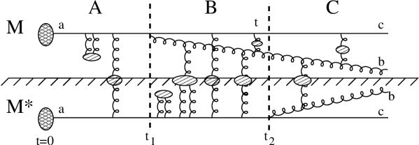
Figure 1: A typical matrix element for gluon emission along with its complex conjugate. The initial blob represents the hard process that creates the hard parton $a$, drawn as a solid line, while the other blobs represent an arbitrary number of plasma particles. There is a monotonic time flow from the left to the right of the diagram which is a consequence of the eikonal approximation. The collision sub-diagrams, or “rungs”, are assumed to have negligible horizontal extent. Only region B actually contributes to the emission process.

Consider, first, elastic collisions in region C (“elastic” refers only to the particles in the jet; the plasma particles could be scattered very inelastically). These collisions will change the momenta of the outgoing particles and typically reduce their energies by a relatively small amount, which will modify their momenta measured in the detector. To discuss the radiation probability, the proper thing to consider is the integrated measurement over the final momenta. This is represented symbolically by the operator

$$\int_{{\bf p}_{b},{\bf p}_{c}}|{\bf p}_{b},{\bf p}_{c}\rangle\otimes\langle{\bf p}_{b},{\bf p}_{c}|=\int d^{2}{\bf x}_{b}d^{2}{\bf x}_{c}~{}|{\bf x}_{b},{\bf x}_{c}\rangle\langle{\bf x}_{b},{\bf x}_{c}|$$ (7)

being convoluted on the right-hand side of the diagram in Figure 1. In the eikonal approximation, this operator is time-independent. To put it as it is, “elastic collisions are elastic”. Hence the sum over states can be performed at time $t_{2}$, making region C irrelevant for the radiation probability. For the same reason, elastic collisions occurring in region A will not affect the emission probability, as they can be absorbed by a change in the jet axis.

Thus only region B contributes. In the eikonal approximation, the object that is evolved in that region is a wavefunction of the form $|{\bf q}_{b},{\bf q}_{c}\rangle\otimes\langle{\bf q}_{a}|$, depending on three transverse momenta. Equivalently, it depends on three transverse positions. This describes the eikonal amplitude times its complex conjugate in region B. Elastic collisions modify all three momenta but preserve the combination $({\bf q}_{b}{+}{\bf q}_{c}{-}{\bf q}_{a})$. In fact, this combination vanishes at all times. Furthermore, it is possible to “gauge” to zero ${\bf q}_{a}$ (or ${\bf q}_{b}$ or ${\bf q}_{c}$) by a rotation of the beam axis AMY . Provided the opening angles are small, this rotation reduces to linear shifts $\delta{\bf q}_{i}\sim p^{+}_{i}$, which commute with both the eikonal expression for the energy $\sim\sum{\bf q}_{i}^{2}/p_{i}$ and with the collision term. Thus this dynamical gauge fixing does not introduce any new term, and the wavefunction really depends on a single transverse momentum. The evolution of this wavefunction will now be expressed in terms of the light-cone Schrödinger equation (2).

Choosing to gauge ${\bf q}_{a}$ to zero so that ${\bf q}\equiv{\bf q}_{b}=-{\bf q}_{c}$, the light-cone energy of the state $|{\bf q}_{b},{\bf q}_{c}\rangle\otimes\langle{\bf q}_{a}|$ is

$$E_{b}{+}E_{c}{-}E_{a}=\frac{p{\bf q}^{2}}{2k(p{-}k)}+\frac{m_{b}^{2}}{2k}+\frac{m_{c}^{2}}{2(p{-}k)}-\frac{m_{a}^{2}}{2p}.$$

This gives $\delta E$ in the Schrödinger equation (2).

The second ingredient in that equation is the collision operator. Quite generally, within the eikonal and instantaneous approximations, the vertical rungs in Figure (1) reduce to a potential

$$-iv({\bf x},\frac{k}{p}{\bf x})$$

added to the Schrödinger equation. This is imaginary, corresponding to a collision rate. Here we have used assumption 4, homogeneity in the transverse plane, to reduce it to a function of two separations, but we could still be left with a quite complicated function of two arguments. To proceed further, we need to make the extra assumption that $v$ is well-described by the dipole-factorized form (2c):

$$\frac{C_{b}{+}C_{c}{-}C_{a}}{2}v_{2}({\bf x})+\frac{C_{a}{+}C_{c}{-}C_{b}}{2}v_{2}(\frac{k}{p}{\bf x})+\frac{C_{a}{+}C_{b}{-}C_{c}}{2}v_{2}(\frac{p{-}k}{p}{\bf x}),$$

for some function $v_{2}({\bf x})$. We believe that this is reasonable. In particular, it was shown in qhatNLO that ${\cal O}(g_{\textrm{s}})$ effects at weak coupling do preserve this form. Perhaps, then, the dominant higher-order effects also do. In momentum space, this assumption implies that the collision operator takes the form (4) for some function $C({\bf q})$.

Since little or no experimental data presently constrains $C({\bf q})$, and since its theoretical determination is so uncertain, at this stage it is probably best to think of the whole curve $C({\bf q})$ as a phenomenological parameter. We shall not have much more to say regarding its choice in this paper.

The final ingredients which enter the diagrams are the hard vertices, which give the DGLAP factor in (1).

This forms the physical basis of the BDMPS-Z formula. Diagrammatically, to obtain our equation (6), one introduces a new time variable $t$ which corresponds to the time of the last scattering before $t_{2}$. The integral over $t_{2}$ can then be performed analytically, since there are no collisions between $t$ and $t_{2}$, and time $t$ becomes the emission time in (6).

III.2 Leading order in the opacity expansion

Gyulassy, Levai and Vitev GLV0 ; GLVmain perform an expansion in the number of in-medium collisions, $N$, occurring during a formation time. Recently, it was shown that this expansion is equivalent to the series expansion of the BDMPS-Z formula (1) in powers of $\mathcal{C}$ Wicks08 . Furthermore, its numerical evaluation appears to converge up to $N=9$. In that sense the GLV expansion is equivalent to the BDMPS-Z formula. Our equation (6) provides an exact and numerically tractable implementation of BDMPS-Z, and its series approximation is thus guaranteed to agree with the GLV series. For what follows it will be useful to highlight the $N=1$ limit, which will be shown to work very well in certain regimes.

In the $N=1$ approximation, $K$ reduces to the free Schrödinger propagator, reducing (6) to

$$\frac{d\Gamma^{a}_{bc}(t)}{dk} \to \frac{P^{a(0)}_{bc}(x)p}{4\pi k^{2}(p{-}k)^{2}}\int_{{\bf p}}\left[\frac{{\bf p}}{\delta E({\bf p})}\right]\mathcal{C}\left[{\bf p}{\rm Re}\,i\int_{0}^{t}dt_{1}e^{-i\delta_{E}({\bf p})(t{-}t_{1})}\right]$$ (8)

$$\equiv \frac{P^{a(0)}_{bc}(x)p}{4\pi k^{2}(p{-}k)^{2}}\int_{{\bf q},{\bf p}}C({\bf q})\frac{1-\cos(\delta E({\bf p})t)}{\delta E({\bf p})}\times\left[\frac{C_{b}{+}C_{c}{-}C_{a}}{2}\left(\frac{{\bf p}^{2}}{\delta E({\bf p})}-\frac{{\bf p}{\cdot}({\bf p}{-}{\bf q})}{\delta E({\bf p}{-}{\bf q})}\right)+\mbox{2 terms}\right].$$

The “2 terms” in the square bracket refer to the last two terms in (4). If we drop the thermal masses in $\delta E$ and make the soft gluon approximation (small $k$), under which the bracket simplifies considerably, this precisely reduces to Eq. (113) of Ref. GLVmain .

In the following, we will refer to (8) (including thermal masses and without making the soft gluon approximation) as the $N=1$ approximation. It is straightforward to evaluate numerically, and it will be seen to be valid at small times.

A word about the collision kernel is in order. GLV conventionally use the “static scattering centers” approximation in which

$$C({\bf q})=\frac{g_{\textrm{s}}^{4}\sum C_{i}n_{i}/d_{i}}{({\bf q}^{2}{+}\mu^{2})^{2}}$$ (9)

with $n_{i}$, $C_{i}$ and $d_{i}$ being the number density, Casimir, and the representation dimension of various plasma constituents. This is a static Yukawa potential, with screening scale $\mu$. In general, this gets modified by recoil effects, which enhance the elastic cross-sections. As has been verified recently in great detail djordjevic (in the $N=1$ case, but with a plausible argument for the general case), a simple change of $C({\bf q})$ to Eq. (12) given below will fully account for this effect. In fact, this particular finding of djordjevic is a consequence of the general argument we have presented above, since the assumptions made in djordjevic are not more general than the ones we have considered. This result is perfectly in line with the viewpoint advocated in the present paper, which is to view $C({\bf q})$ as a phenomenological input to the formalism. In this work we will only use the collision term (12) below.

III.3 AMY

Some work has been done, relating the finite-temperature approach of Arnold-Moore-Yaffe (AMY) to that outlined in section II.1, in Ref. aurzak and independently in Ref. arnoldexact . Other recent work on the AMY formalism includes SV . The computation in the present subsection is very similar to those in Refs. aurzak ; arnoldexact . In both references, the key step was to re-express BDMPS-Z in terms of a rate. This is also the idea behind (6). It is tantamount to formulating AMY in coordinate space. AMY consider bremsstrahlung from an homogeneous medium of infinite length and neglect effects associated with the jet production time $t=0$ as well as effects resulting from changes of the medium during a formation time. For the brick problem, this means that AMY should be valid in the large $t$ limit.

Our formulation connects very naturally with that of AMY. In the large $t$ limit (6) becomes

$$\frac{d\Gamma^{a}_{bc}}{dk}\to\frac{P^{a(0)}_{bc}(x)p}{4\pi k^{2}(p{-}k)^{2}}\times{\rm Re}\,\int_{{\bf p}}{\bf f}({\bf p}){\cdot}{\bf p},\quad{\bf f}({\bf p})\equiv\frac{4k^{2}(p{-}k)^{2}}{p^{2}}\int_{-\infty}^{0}dt_{1}\int_{\bf q}\frac{i{\bf q}}{\delta E({\bf q})}\circ\mathcal{C}\circ K(0,{\bf q};t_{1},{\bf p}).$$ (10)

Now we observe that

$${\bf f}({\bf p})+\frac{{\bf p}}{i\delta E}\equiv\tilde{\bf f}({\bf p})=\frac{4k^{2}(p{-}k)^{2}}{p^{2}}\int_{-\infty}^{0}dt_{1}\int_{\bf q}{\bf q}K(0,{\bf q};t_{1},{\bf p})$$

has the same real part as ${\bf f}({\bf p})$. By time-translation invariance, $\tilde{\bf f}({\bf p})$ obeys the steady-state equation

$$\left[i\delta E+\mathcal{C}\right]\tilde{\bf f}({\bf p})={\bf p}$$ (11)

which suffices to determine it. Eqs. (10) and (11) are precisely equations (10) and (11) appearing in JeonMoore . Hence the rate which we have defined agrees precisely with that defined by AMY when $t\gg t_{\textrm{form}}$.

It is sometimes stated that the AMY treatment, being rigorously justified in thermal field theory in the limit of small coupling, can be valid only for weakly coupled plasmas. This is incorrect. We see that this treatment will always be valid at times larger than a formation time, within the rather general assumptions discussed in section III.1. On the other hand, a rigorous application of AMY does suggest the use of

$$C({\bf q})=\frac{g_{\textrm{s}}^{2}m_{\textrm{D}}^{2}T}{{\bf q}^{2}({\bf q}^{2}{+}m_{\textrm{D}}^{2})},\quad\quad\mbox{with $m_{\textrm{D}}^{2}=\frac{3}{2}g_{\textrm{s}}^{2}T^{2}$ in QCD},$$ (12)

as the collision kernel. This expression is obtained at leading-order in the coupling in thermal field theory. (This was first obtained in this form in AGZ .) This is the only place where a weakly coupled plasma is actually needed, when $k\gg T$ and the conditions of section III.1 are satisfied. Otherwise, if the plasma is not truly weakly coupled but the jet still is, corrections to (12) are to be expected.

III.4 The deep LPM regime: The harmonic oscillator

At asymptotically high energies $p,k\gg T$ the deep LPM regime is realized, in which a large number of collisions occurs during a formation time. This motivates a diffusion approximation in which the Hamiltonian becomes

$$H=\tilde{m}_{\textrm{eff}}+\frac{p{\bf p}^{2}}{2k(p{-}k)}+\frac{i\hat{q}_{3}}{4}\frac{\partial}{\partial{\bf p}}{\cdot}\frac{\partial}{\partial{\bf p}},$$ (13)

where $\tilde{m}_{\textrm{eff}}=\frac{m_{b}^{2}}{2k}+\frac{m_{c}^{2}}{2(p{-}k)}-\frac{m_{a}^{2}}{2p}$. The effective diffusion coefficient $\hat{q}_{3}$ is related to the quark momentum broadening coefficient through $\hat{q}_{3}=\frac{\hat{q}_{q}}{C_{\textrm{F}}}\left[\frac{C_{b}{+}C_{c}{-}C_{a}}{2}+\frac{C_{a}{+}C_{c}{-}C_{b}}{2}\frac{k^{2}}{p^{2}}+\frac{C_{a}{+}C_{b}{-}C_{c}}{2}\frac{(p{-}k)^{2}}{p^{2}}\right]$, where $\hat{q}_{q}$ is defined as

$$\hat{q}_{q}=\int^{{\bf q}_{\textrm{max}}}d^{2}{\bf q}~{}{\bf q}^{2}\frac{d^{2}\Gamma_{\textrm{el}}}{d^{2}{\bf q}}=\frac{4}{3}\int_{\bf q}^{{\bf q}_{\textrm{max}}}{\bf q}^{2}C({\bf q}).$$ (14)

This Hamiltonian is that of a harmonic oscillator with complex frequency $\omega_{0}=\sqrt{\frac{-i\hat{q}_{3}p}{2k(p{-}k)}}$. This means that it can be solved analytically. For a homogeneous brick the exact solution is

$$K(t,{\bf q};t_{1},{\bf p})=\frac{p^{3}}{4k^{3}(p{-}k)^{3}}\frac{1}{2\pi i\omega_{0}\sin\omega_{0}(t{-}t_{1})}\exp\left({i\frac{p[({\bf q}^{2}{+}{\bf p}^{2})\cos\omega_{0}(t{-}t_{1})-2{\bf p}{\cdot}{\bf q}]}{2k(p{-}k)\omega_{0}\sin\omega_{0}(t{-}t_{1})}-i\tilde{m}_{\textrm{eff}}(t{-}t_{1})}\right).$$

Upon performing the ${\bf p}$ integration in the rate (6) and changing variable to $u\propto{\bf q}^{2}$, we obtain

$$\frac{d\Gamma^{a}_{bc}}{dk}\to\frac{P^{a(0)}_{bc}(x)}{4\pi^{2}k(p{-}k)}\times{\rm Re}\,\frac{-\hat{q}_{3}(t)m_{\textrm{eff}}}{\omega_{0}}\int_{0}^{t}dt^{\prime}\frac{e^{-i\tilde{m}_{\textrm{eff}}t^{\prime}}\sin\omega_{0}t^{\prime}}{\cos^{3}\omega_{0}t^{\prime}}\int_{0}^{\infty}\frac{udu~{}e^{-u}}{(u+i\frac{m_{\textrm{eff}}}{\omega_{0}}\frac{\sin\omega_{0}t^{\prime}}{\cos\omega_{0}t^{\prime}})^{3}}.$$ (15)

It can be shown that denominators are always non-singular.

The brick result, Eq. (15), will suffice for the present paper. Possibly, similar formulae for evolving media could be derived following the methods of arnoldexact . We will refer to (15) as the “multiple soft scattering” approximation.

It is unusual to express results obtained within this approximation in terms of a rate, and, for this reason, (15) may appear unfamiliar to many readers. We insist to use a rate in order to facilitate its comparison with (6) later on. To see that (15) is indeed totally equivalent to the usual results, consider, for instance, its limit as $m_{\textrm{eff}}\to 0$:

$$\frac{d\Gamma^{a}_{bc}}{dk}\to\frac{P^{a(0)}_{bc}(x)}{8\pi^{2}k(p{-}k)}\times\hat{q}_{3}(t)~{}{\rm Re}\,\int_{0}^{t}dt^{\prime}\frac{i}{\cos^{2}(\omega_{0}t)}=\frac{P^{a(0)}_{bc}(x)}{4\pi^{2}p}\times{\rm Re}\,\left[-\omega_{0}\tan\omega_{0}t\right].$$ (16)

This is the time derivative of the familiar BDMPS formula $\frac{dP^{a}_{bc}}{dk}=\frac{P^{a(0)}_{bc}(x)}{4\pi^{2}p}\ln|\cos\omega_{0}t|$, hence it is completely equivalent to it. More generally, when masses are included, we expect complete agreement with the formulae of ZakharovL .

Physically, this approximation is justified when a large number of soft collisions occur during a formation time. While this is formally the case in the high-energy limit, the corresponding expansion parameter is only $1/\log(E)$ arnolddogan . We will nevertheless verify that this approximation is accurate in the regime of high energy and sufficiently large time. At times smaller than a formation time, however, this approximation is not well motivated since a large number of collisions may not be reached. This was emphasized in zakharov2000 ; arnold . In particular, in arnold it is explained that formation time effects are only well described in a relatively restricted time window of parametric size $\sqrt{\log(E/T)}$. This quantity is not large at RHIC (nor will it be at the LHC), and its smallness will become apparent numerically below.

IV Multiple emissions

So far we have discussed how to calculate the rate at which a single quanta is radiated. One advantage of a rate formulation is that it is obvious how to account for multiple emissions: One simply writes down a “rate equation.”

In this section we keep the notation general, in anticipation of situations in which the local plasma frame will be evolving with time. Hence we work entirely in the lab frame. In general, the evolution of the distribution of quarks and gluons within a jet may be described within the Boltzmann framework

$$\frac{dn_{q}(p)}{dt}\! = \!\!\int dk\left[n_{q}(p{+}k)\frac{d\Gamma^{q}_{qg}(p{+}k,k)}{dk}+2n_{g}(p{+}k)\frac{d\Gamma^{g}_{qq}(p{+}k,k)}{dk}-n_{q}(p)\frac{d\Gamma^{q}_{qg}(p,k)}{dk}\theta(p{-}k)\right]$$

$$+\textrm{[elastic]}+\textrm{[vacuum]},$$

$$\frac{dn_{g}(p)}{dt}\! = \!\!\int dk\left[n_{q}(p{+}k)\frac{d\Gamma^{q}_{gq}(p{+}k,k)}{dk}+n_{g}(p{+}k)\frac{d\Gamma^{g}_{gg}(p{+}k,k)}{dk}-n_{g}(p)\left(\frac{d\Gamma^{g}_{qq}(p,k)}{dk}\theta(p{-}k)+\frac{d\Gamma^{g}_{gg}(p,k)}{dk}\theta(p{-}2k)\right)\right]$$ (17)

$$+\textrm{[elastic]}+\textrm{[vacuum]},$$

where the $k$ integrations run from 0 to $\infty$. The rate $d\Gamma^{a}_{bc}/dk(p,k)$ for emission of parton $b$ with energy $k$ from parent parton $a$ with energy $p$ is as defined by (6). In an evolving medium its computation is described in the Appendix A. Our notation follows that of JeonMoore , although the integration region is different; JeonMoore and other AMY-based treatments typically include absorption processes from the medium. The reason we omit these processes will be explained below.

The “elastic” component accounts for the energy lost by collisions against plasma constituents. It has been extensively discussed in the literature elastic , and we will not do so here. We only mention that this component is important when discussing observables such as $R_{AA}$ qin .

It is obvious that a vacuum component has to be included. This component, however, deserves further comment. We must recall what is already included in $d\Gamma^{a}_{bc}/dk(p,k)$. This is the vacuum-subtracted rate (6) which includes all interference effects between vacuum and medium radiation. What is left is precisely the amount subtracted in (5) corresponding to the vacuum radiation, which may be written

$$\frac{dP^{a,\textrm{vac}}_{bc}}{dk}=\frac{P^{a(0)}_{bc}(x)}{2\pi p}\times\int_{{\bf q}}{\bf q}^{2}\left|\frac{p}{2k(p{-}k)}\int_{0}^{\infty}dte^{-i\int_{0}^{t}\delta E}\right|^{2}.$$ (18)

In the absence of thermal and vacuum masses, the integral is $\int_{{\bf q}}\frac{1}{{\bf q}^{2}}$ which is the standard collinear logarithm for vacuum radiation. But because thermal masses are nonzero, (18) describes the probability for vacuum radiation with a slight suppression due to the thermal masses. This suppression is known as the (thermal) Ter-Mikaelian effect and it has been analyzed in the RHIC context in adilhorowitz ; djordjevicter . We will not discuss it further here.

The single-emission probability (18) is to be exponentiated so as to maintain a reasonable ordering of events; by our notation we do not wish to suggest that the vacuum radiation can be naturally handled as a rate. Some vacuum radiation will occur before or overlap with the earliest medium radiation, and some will be fragmentation radiation occurring afterwards in the confined phase. We hope to return to this question of ordering in a future work. For the application we have in mind in this work, we return to our idealized thermal medium, and concentrate on the radiative component $d\Gamma^{a}_{bc}/dk$.

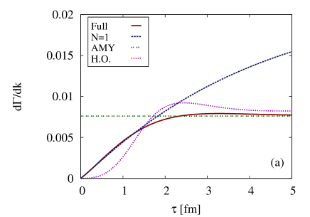
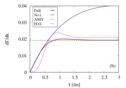
Figure 2: (Color online) Radiation rate for a 3 GeV gluon from a 16 GeV parent quark as a function of travelled length since the birth of the jet. The medium is a uniform brick of QGP at $T=0.2$ GeV (panel (a)) and $T=0.4$ GeV (panel (b)), with $\alpha_{\textrm{s}}=0.3$.

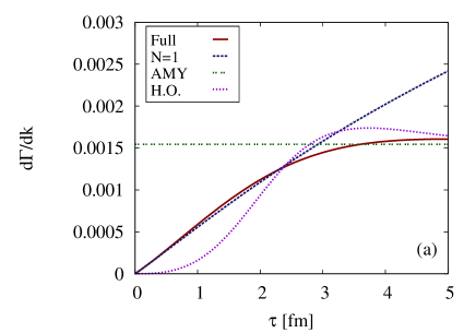
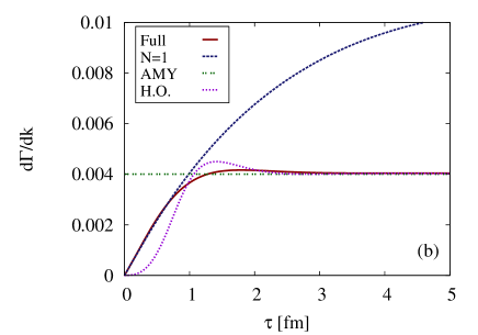
Figure 3: (Color online) Same as Figure 2 but for a 8 GeV gluon radiated from a 16 GeV quark.

V Results and discussion

In this section, we calculate the scattering rates in different approaches and compare the results. Specifically, we compare results obtained with the formalism presented here, in which the formation time/length is included explicitly, with those obtained to first order in the opacity expansion, with AMY, and in the multiple soft scattering approximation. The first such comparison is shown in Figure 2.

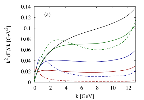
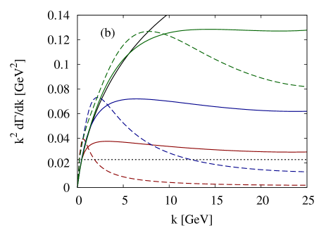
Figure 4: (Color online) “Instantaneous” radiation spectra $k^{2}d\Gamma/dk$ in a $T=0.2$ GeV brick for three different times. Panel (a): Gluons radiated from a 16 GeV parent quark, at times 0.5 fm/c (red), 1.0 fm/c (blue), and 1.5 fm/c (green). The solid line shows the results of our full calculation, the dashed line the result of multiple soft scatterings, and the dotted line shows the results of purely elastic scatterings. Panel (b): Same as panel (a), but for a 50 GeV parent quark. Times are 0.8 fm/c (red), 1.6 fm/c (blue), and 3.2 fm/c (green). In both panels, results obtained with AMY are shown as a black solid line.

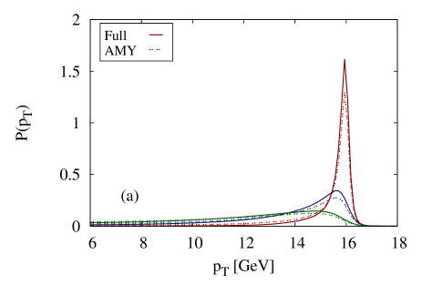
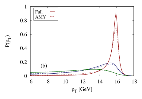
Figure 5: (Color online) Degradation of quark transverse momentum as a function of time for two QGP bricks at $T=0.2$ GeV (panel (a)), and $T=0.4$ GeV (panel (b)). Both initial distributions are delta-functions at 16 GeV and are not shown. The three distributions correspond to three different final times. From right to left those are: 1, 3, and 5 fm/c for panel (a), and 0.5, 1.5, 2.5 fm/c for panel (b).

AMY is seen to be valid for large times, and our results do tend to that limit as $\tau\to\infty$: A satisfying consistency check. There is a slight overshoot at a finite time, followed by asymptotic convergence, which we interpret as a gradual setting in of the LPM suppression. The left panel of Figure 2 shows the differential rate at which a 3 GeV gluon would be radiated off a 16 GeV quark in a “brick” of equilibrated quark-gluon plasma at a fixed temperature of $T=0.2$ GeV. The right panel represents results for similar requirements, but for a temperature of 0.4 GeV. For the coupling constant we used $\alpha_{\textrm{s}}=0.3$, which is similar to the value found from experiment in bass based on the AMY framework. Figure 3 is a repetition of this exercise with different kinematics: a 16 GeV quark now radiates a 8 GeV gluon. In both cases, note that the rates obtained here smoothly interpolate between those obtained at leading order in the opacity expansion and those produced by AMY.

The $N=1$ approximation, Eq. (8), is seen to accurately track the full result at small times. It begins to deviate at roughly the formation time, due to the onset of the Landau-Pomeranchuk-Midgal (LPM) interference effect between multiple scatterings occurring in the medium. The difference between the $N=1$ and full curves precisely accounts for that effect. The amount of that difference is proportional to the number of collisions occurring during a formation time and can thus be used to estimate it: for RHIC energies, we thus estimate that $1\lesssim N\lesssim 3$, typically. Higher orders in the opacity expansion have been discussed in Wicks08 ; we have not compared with these results.

The linear rise of rates at small time is thus to be interpreted within the $N=1$ approximation. At small times, the virtuality of the jet is very high and only very hard collisions contribute. In this region, (8) may be estimated as

$$d\Gamma/dk\approx P^{(0)}/p\int_{{\bf q}_{\textrm{min}}}^{\infty}C({\bf q})\propto P^{(0)}g^{4}n/p\,{\bf q}^{2}_{\textrm{min}}$$ (19)

where ${\bf q}^{2}_{\textrm{min}}\sim k/\tau$ and $n$ is a number density of charge carriers. This produces the linear rise. This exhibits that the relevant collisions are harder than the plasma scale, and therefore more weakly coupled, making this region a robust prediction of QCD.

In Fig 4 we indicate the radiation spectrum $k^{2}d\Gamma/dk$ as a function of $k$ in a brick of temperature $T=0.2$ GeV, for a $16$ GeV parent quark with the same parameters as above. As time increases, the curves move upwards and eventually saturate the (time-independent) AMY prediction. In the left panel, this saturation occurs at approximately $t=3.5$ fm/c. To avoid making the figures too busy, we have omitted the $N=1$ spectra. The $N=1$ spectra are indistinguishable from the full curve when the formation time effects are important, on the right-hand side of the figures (below the AMY curve), but they keep growing and overshoot the AMY asymptote on the left in keeping with Figures 2 and 3.

Regarding multiple soft approximation, it is important to distinguish between the small and large time regions. At large times the approximation performs rather well as it tracks closely the AMY result. It produces slightly red spectra as may be seen in Figure 4 but also in Figure 2, where the oscillator curves asymptote to slightly higher values. The oscillator curves depend on a phenomenological parameter $\hat{q}_{q}$ which we have determined, for both temperatures, by requiring the correct radiation rate when $k=8$. That is, the asymptotic agreement in Figure 3 is a consequence of our choice of $\hat{q}_{q}$. The values we have used are $\hat{q}_{q}=0.37$ GeV²/fm and $2.45$ GeV²/fm at $T=0.2$ GeV and $T=0.4$ GeV, respectively. These values should be compared with the definition of $\hat{q}_{q}$ (14). For the collision kernel Eq. (12), the latter evaluates to

$$\hat{q}_{q}=\frac{g^{2}m_{D}^{2}T\log(1+\frac{q_{\textrm{max}}^{2}}{m_{D}^{2}})}{3\pi}.$$ (20)

Plugging in $q_{\textrm{max}}\sim 3$ and 4 GeV respectively (estimated from twice the values [twice is for $2=p/k$] entering the transverse momentum spectra in Figure 6) leads to $\hat{q}_{q}\approx 0.33$ GeV²/fm and $2.0$ GeV²/fm respectively. We conclude that, in the large $t$ region, the values of $\hat{q}$ required by the oscillator model may be larger than those corresponding to the quark momentum broadening problem but only by a small amount $\stackrel{{\scriptstyle<}}{{{}_{\sim}}}20\%$.

In the small $t$ region, the multiple soft scattering approximation performs poorly and does not reproduce the full result (which it is supposed to approximate). This is seen in Figures 2 and 3 at small times, and is also is also obvious from Figure 4 where the ultraviolet part of the spectrum is absent at small times. In general, whenever the “Full” and “AMY” curves differ, meaning that interference between vacuum and medium radiation occurs, the corresponding suppression is exaggerated by the multiple soft scattering approximation. Analytically, at fixed $p$ and $k$, the rate in the multiple soft scattering approximation grows like $t^{3}$ at small times while the correct, $N=1$, rate rises like $t$. This qualitative feature has been anticipated in the above-mentioned work zakharov2000 ; arnold . Finally, we note that in all regions our “multiple soft approximation” curves differ by only a very small amount from those obtained within the more familiar massless approximation Eq. (16). All our conclusions thus apply also to the latter, simpler formula.

Our choice to plot the combination $k^{2}d\Gamma/dk$ is motivated by the fact that this provides a good estimate for $dE/dt=\int kdkd\Gamma/dk$, which is the relevant concept to discuss the soft region. In particular, this quantity is infrared-safe. At larger values $k\stackrel{{\scriptstyle>}}{{{}_{\sim}}}2\div 3$ GeV (corresponding to the lateral shift of the measured leading-hadron spectra $dN\sim dp_{\perp}/p_{\perp}^{8.1}$ for $R_{AA}\sim 0.2$), $dE/dt$ ceases to be a useful concept and the more appropriate quantity is $kd\Gamma/dk$. We have included on the figure the leading-order elastic rate

$$\frac{d\Gamma_{\textrm{el}}}{dk}=\frac{g^{2}m_{D}^{2}C_{F}}{16\pi k^{2}}$$ (21)

as extracted from Thoma91 . Note that there is no kinematic cutoff on the amount of longitudinal energy which can be lost through elastic scattering. To the best of our understanding, elastic processes are not interference-suppressed at small times and so, in the brick problem, produce a time-independent contribution. As a function of the temperature, we find that the elastic component dominates the radiative one for $k<2.5T$.

This may be interpreted in two ways. First, this means that the elastic component is only important in the soft region, which is the standard lore. Second, this implies that soft radiation is largely irrelevant. Indeed, since there is no invariant way to distinguish soft emission processes from collisional ones, the best way to look at radiation with $k\ll 2.5T$ is as a small, sub-leading correction to the elastic component. This is relevant because (6) was never meant to be accurate in this region anyway. This is also why we have not included medium absorption processes, as well as Bose-stimulation or Pauli-blocking factors, in (17) – all these processes account for at most a small increase in the elastic component.

In addition, it is instructive to study the efficiency with which the medium knocks apart the initial delta function, starting for example from a 16 GeV quark. This is shown in the two panels of Figure 5, for two different brick temperatures. At the later times, any hint of a peak structure has mostly been washed out. Notably, the inclusion of the formation time effects does reduce the distribution in magnitude, but does not introduce any significant shape distortion.

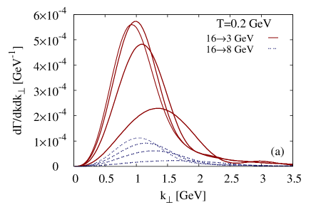
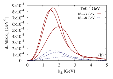
Figure 6: (Color online) Transverse momentum distribution of 3 GeV and 8 GeV gluons radiated from a 16 GeV parent quark. Panel (a) is for a QGP brick at $T=0.2$ GeV. From right to left the gluons are emitted at times 1, 2, 3 and 5 fm/c. Panel (b) is for a QGP brick at $T=0.4$ GeV and times 0.5, 1 and 2 fm/c.

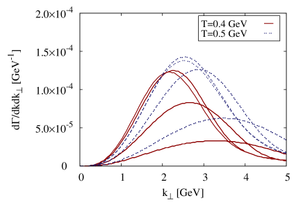
Figure 7: (Color online) Transverse momentum distribution of a 10 GeV gluon radiated from a 50 GeV quark at $T=0.4$ GeV and $T=0.5$ GeV: Conditions of some relevance for the LHC. From right to left, times are 0.5, 1, 2, and 3 fm/c.

To address the self-consistency of the formalism it will be important to look at the $k_{\perp}$ distribution of the radiated gluons. This is shown in Figure 6. It is difficult to draw any firm conclusion regarding this issue in the RHIC context at present since in this paper we have focused on a semi-realistic brick problem. Nonetheless, in the cases indicated we are satisfied that the relevant values of $k_{\perp}$ are always smaller than the energy $k$ of the gluon. In the worst case we have considered, corresponding to a 3 GeV gluon radiated from a 16 GeV parent quark in a $T=0.4$ GeV brick, the typical opening angle from $k_{\perp}/k$ is approximately $30^{\circ}$. In other cases it is much smaller. The collinear approximation should thus be under control in the cases shown in this paper. The $k_{\perp}$ scale is mostly determined by the temperature of the medium, although $k$ also plays a role (this is in qualitative agreement with the parametric estimate $k_{\perp}\sim(\hat{q}k)^{1/4}$ in the deep LPM regime). The $k_{\perp}$ scale in the figure gives the scale at which the running coupling is to be evaluated (up to an unknown multiplicative factor whose determination would require a full 1-loop computation), which should be useful for the reliable inclusion of running coupling effects in the future. In many cases the $k_{\perp}$’s relevant at RHIC are seen not to be much larger than 1 GeV, suggesting a possible importance of loop corrections. On the other hand, strong non-perturbative effects would appear unlikely at such transverse momentum scales. The situation on all these issues is expected to improve under LHC conditions, as shown in Figure 7.

VI Conclusion

We have described a method to solve exactly the BDMPS-Z radiation formula. The key step in this method is the focus on a differential radiation rate Eq. (6), which is both numerically tractable and physically meaningful. Such a rate formulation immediately connects with the AMY formalism. On the other hand, this rate is constructed in such a way that its time integral agrees precisely with the radiation probability previously defined by BDMPS-Z, including in situations in which the duration of the emission process is not negligible and where the AMY treatment was previously not applicable. This includes interference effects between medium and vacuum radiation. The method makes it possible to study numerically and exactly, for the first time, BDMPS-Z radiation spectra in all kinematic regimes. The rate formulation makes the transitions between different regimes particularly easy to see.

In the brick problem, we have distinguished two different interference-dominated regimes. In the first one, occurring at small time, the medium modifications to the radiation are determined by interference between the vacuum radiation and that produced by a single hard collision. This regime smoothly connects with a second one, in which the vacuum radiation becomes irrelevant and the radiation is determined by Landau-Pomeranchuk-Migdal (LPM) interference between in-medium radiation. The latter regime is well described both by AMY and by the multiple soft scattering approximation, while the former regime is well described by the GLV $N=1$ approximation. The transition between these two regimes occurs at a physically important length scale, $t\sim 1\div 2$ fm depending upon the energies, which makes it essential to accurately describe it.

Generally speaking, for a given medium we have shown that AMY (in previous implementations) over-estimates radiation while the multiple soft scattering approximation systematically under-estimates it. This agrees qualitatively with the pattern of interaction rates which have been extracted from experiment in the past using those models bass .

Phenomenologically speaking, information about the underlying medium enters exactly two places in the present formalism. One is the elastic collision rate $d^{2}\Gamma_{\textrm{el}}({\bf q})/d^{2}{\bf q}$, related to the quantity $C({\bf q})$ in this paper, and the other is the thermal masses. Although we have made no detailed investigation of the effect of thermal masses it seems clear that the most important parameter is the elastic collision rate. For a plasma isotropic in its rest frame, this is a function of $|{\bf q}|$ which is independent of the jet energy. Our analysis shows that its second moment, $\hat{q}_{q}$, does not suffice to characterize jet energy loss as it ignores a hard Coulomb tail which dominates at small times. In the present paper we have contented ourselves with the simplest available choice, Eq. (12), but it will be important in the future to learn more about the phenomenological implications of the shape of this curve.

It is known that current efforts to extract meaningful physics from jet quenching measurements in heavy ion collisions have to be done with the help of hydrodynamic modelling. The formation time effects discussed in the present paper are expected to be particularly relevant for non-central collisions, and for angular correlation measurements, where the details of the geometry of the emitting region play a larger role. As a consequence, a systematic analysis of several different observables will be needed to quantitatively characterize the hot and dense strongly interacting medium formed at RHIC, and soon to be created at the LHC.

VII acknowledgements

It is a pleasure to thank Néstor Armesto, Peter Arnold, Sangyong Jeon, Abhijit Majumder, Guy D. Moore, Carlos Salgado, Björn Schenke, and Urs Wiedemann for discussions. This work was funded in part by the Natural Sciences and Engineering Research Council of Canada, and in part (SCH) by NSF grant PHY-0503584.

Appendix A Computing the radiation in an expanding medium

In this appendix, we spell out, for future reference, the proper formulae to be used in expanding media. The formula will also be valid in the situations in which the medium is not homogeneous in the longitudinal direction over a formation time. The derivation follows the discussion in section III.1, where longitudinal homogeneity was indeed never required.

The generalization of (6) in this case is

$$\frac{d\Gamma^{a}_{bc}(t)}{dk}\equiv\frac{P^{a(0)}_{bc}(x)}{\pi p}\times{\rm Re}\,\int_{0}^{t}dt_{1}\int_{{\bf q},{\bf p}}\frac{i{\bf q}}{\overline{\delta E}({\bf q},t)}\tilde{\gamma}(t)\,\mathcal{C}(t)\,K(t,{\bf q};t_{1},{\bf p})\cdot{\bf p}.$$ (22)

In this expression $i/{\overline{\delta E}({\bf q},t)}=\int_{t}^{\infty}dt^{\prime}e^{-i\int_{t}^{t^{\prime}}\delta E}$. (This will always be very close to $i/\delta E({\bf q},t)$, provided thermal masses change slowly.)

Equation (6) contains the time-dilation factor $\tilde{\gamma}(t)\equiv\frac{E_{\textrm{plasma}}}{E_{\textrm{lab}}}$. It describes the transformation of $d^{2}\Gamma_{\textrm{el}}/d^{2}{\bf q}$ from the plasma frame to the lab frame. This factor always multiply the operator $\mathcal{C}$. If, in the lab frame, the plasma is moving with velocity $v$ and at angle $\theta$ relative to the jet axis, this factor may be written

$$\tilde{\gamma}=\frac{1-v\cos\theta}{\sqrt{1-v^{2}}}.$$

The expression (4) for the now time-dependent $\mathcal{C}$ is not otherwise modified and $C({\bf q})$ entering it should be computed in the plasma frame as usual.

The same factor multiply $\mathcal{C}$ in the equation for $K$ which now reads

$$\left[\partial_{t}+i\delta E({\bf q},t)+\tilde{\gamma}(t)\mathcal{C}(t)\right]K(t,{\bf q};t_{1},{\bf p})=0,\quad K(t_{1},{\bf q};t_{1},{\bf p})=\frac{p^{2}}{4k^{2}(p{-}k)^{2}}(2\pi)^{2}\delta^{2}({\bf q}-{\bf p}).$$ (23)

The expression for the light-cone energy is unchanged

$$\delta E({\bf q},t)=\frac{p{\bf q}^{2}}{2k(p{-}k)}+\frac{m_{b}^{2}(t)}{2k}+\frac{m_{c}^{2}(t)}{2(p{-}k)}-\frac{m_{a}^{2}(t)}{2p}$$ (24)

provided all energies in it are measured in the lab frame. For heavy quarks, the masses are the rest masses, while for light quarks and gluons the masses are the asymptotic thermal masses (respectively $m_{\infty}^{2}=\frac{g_{\textrm{s}}^{2}T^{2}}{3}$ and $m_{\infty}^{2}=\frac{3g_{\textrm{s}}^{2}T^{2}}{4}$ in QCD at leading order in thermal perturbation theory).

The solution to these equations exhibits, in an evolving medium, in addition to the finite-size effects discussed in the present paper, important memory effects. Their analysis lies outside our present scope.

We briefly describe our numerical implementation of (22). We view $K(t;t_{1})$ as an evolution operator in $t_{1}$ starting from time $t$. (Since $t_{1}<t$, the evolution time is $|t_{1}{-}t|$.) The initial wavefunction at time $t$ is the vector-valued function $\vec{\psi}({\bf p},|t_{1}{-}t|{=}0)=\tilde{\gamma}(t)\mathcal{C}(t)\circ\frac{i{\bf p}}{\overline{\delta E}({\bf p},t)}$. We evolve it numerically in the “interaction picture” as

$$\frac{\partial}{\partial|t_{1}{-}t|}\vec{\psi}_{I}({\bf p},|t_{1}{-}t|)=-e^{i\int_{t_{1}}^{t}\delta E({\bf p})}\tilde{\gamma}(t_{1})\mathcal{C}(t_{1})e^{-i\int_{t_{1}}^{t}\delta E({\bf p})}\vec{\psi}_{I}({\bf p},|t_{1}{-}t|)$$

Going to the interaction picture removes violent phases from $\vec{\psi}_{I}$. The initial conditions at time $t$ decay at large ${\bf p}$ like $\vec{\psi}_{I}\sim{\bf p}C({\bf p})\sim{\bf p}/{\bf p}^{4}$. This decay is preserved at all times. To find $\Gamma$ we need to take the integral $\int_{{\bf p}}\int dt_{1}e^{-i\int_{t_{1}}^{t}\delta E({\bf p})}\,{\bf p}{\cdot}\vec{\psi}_{I}({\bf p},|t_{1}{-}t|)$. Because the ${\bf p}$ integral is not absolutely convergent, it is most convenient to perform the $t_{1}$ integration first. At large times, $\psi_{I}$ tends to zero and the time integral saturates. However, oscillations in time will cause an extra suppression $\sim 1/\delta E({\bf p})$ at large ${\bf p}$ making the ${\bf p}$ integration convergent, as it should be expected physically. Rotational invariance in the ${\bf p}$ plane can be used to set $\vec{\psi}_{I}=\frac{{\bf p}}{{\bf p}^{2}}\tilde{\psi}_{I}(|{\bf p}|)$ for some scalar function $\tilde{\psi}_{I}(|{\bf p}|)$.

References

- (1) M. Gyulassy and L. McLerran, Nucl. Phys. A750, 102 (2005); J. Adams et al., ibid., 184 (2005); I. Arsene et al.,, ibid. 1 (2005); B. B. Back et al., 28 (2005).
- (2) K. Adcox et al., Phys. Rev. Lett. 88, 022301 (2002); C. Adler et al., Phys. Rev. Lett. 89, 202301 (2002).
- (3) M. Gyulassy and X.-N. Wang, Nucl. Phys. B420, 583 (1994).
- (4) See, for example, E. Shuryak, Prog. Part. Nucl. Phys. 62, 48 (2009), and references therein.
- (5) L. D. Landau and I. Pomeranchuk, Dokl. Akad. Nauk Ser. Fiz. 92 (1953) 535; L. D. Landau and I. Pomeranchuk, Dokl. Akad. Nauk Ser. Fiz. 92 (1953) 735; A. B. Migdal, Dokl. Akad. Nauk S.S.S.R. 105, 77 (1955); A. B. Migdal, Phys. Rev. 103, 1811 (1956).
- (6) TEC-HQM Collaboration, in preparation.
- (7) S. A. Bass, C. Gale, A. Majumder, C. Nonaka, G. Y. Qin, T. Renk and J. Ruppert, Phys. Rev. C 79, 024901 (2009).
- (8) P. Arnold, G. D. Moore, and L. G. Yaffe , JHEP 0111 057 (2001); 0112, 009 (2001); 0206, 030 (2001).
- (9) S. Jeon and G. D. Moore, Phys. Rev. C 71, 034901 (2005) [arXiv:hep-ph/0309332].
- (10) G. Y. Qin, J. Ruppert, C. Gale, S. Jeon and G. D. Moore, Phys. Rev. C 80, 054909 (2009) [arXiv:0906.3280 [hep-ph]].
- (11) S. Turbide, C. Gale, E. Frodermann and U. Heinz, Phys. Rev. C 77, 024909 (2008); B. Schenke, C. Gale and G. Y. Qin, Phys. Rev. C 79, 054908 (2009); G. Y. Qin, J. Ruppert, C. Gale, S. Jeon and G. D. Moore, Phys. Rev. C 80, 054909 (2009).
- (12) B. G. Zakharov, JETP Lett. 63 952 (1996) [hep-ph/9607440].
- (13) B. G. Zakharov, JETP Lett. 65, 615 (1997) [hep-ph/9704255].
- (14) R. Baier, Y. L. Dokshitzer, A. H. Mueller, S. Peigne and D. Schiff, Nucl. Phys. B 478, 577 (1996) [arXiv:hep-ph/9604327]; 483, 291 (1997) [arXiv:hep-ph/9607355].
- (15) V. N. Gribov and L. N. Lipatov, Sov. J. Nucl. Phys. 15 (1972) 438; V. N. Gribov and L. N. Lipatov, Sov. J. Nucl. Phys. 15 (1972) 675; L. N. Lipatov, Sov. J. Nucl. Phys. 20 (1975) 94; G. Altarelli and G. Parisi, Nucl. Phys. B126 (1977) 298; Yu. L. Dokshitzer, Sov. Phys. JETP 46 (1977) 641.
- (16) M. Gyulassy, P. Levai and I. Vitev, Nucl. Phys. B 571, 197 (2000) [arXiv:hep-ph/9907461].
- (17) P. Aurenche and B. G. Zakharov, JETP Lett. 85, 149 (2007).
- (18) P. B. Arnold and C. Dogan, Phys. Rev. D 78, 065008 (2008) [arXiv:0804.3359 [hep-ph]].
- (19) S. Caron-Huot, Phys. Rev. D 79, 065039 (2009) [arXiv:0811.1603 [hep-ph]].
- (20) S. M. Aybat, L. J. Dixon and G. Sterman, Phys. Rev. D 74, 074004 (2006) [arXiv:hep-ph/0607309].
- (21) M. Gyulassy, P. Levai and I. Vitev, Nucl. Phys. B 594, 371 (2001) [arXiv:nucl-th/0006010].
- (22) S. Wicks, arXiv:0804.4704 [nucl-th].
- (23) M. Djordjevic and U. Heinz, Phys. Rev. C 77, 024905 (2008) [arXiv:0705.3439 [nucl-th]]; Phys. Rev. Lett. 101, 022302 (2008) [arXiv:0802.1230 [nucl-th]].
- (24) P. Arnold, Phys. Rev. D 79, 065025 (2009) [arXiv:0808.2767 [hep-ph]];
- (25) S. V. Suryanarayana, arXiv:1005.5122 [hep-ph].
- (26) P. Aurenche, F. Gelis and H. Zaraket, JHEP 0205, 043 (2002) [arXiv:hep-ph/0204146].
- (27) P. Arnold, Phys. Rev. D 80, 025004 (2009) [arXiv:0903.1081 [nucl-th]].
- (28) B. G. Zakharov, JETP Lett. 73, 49 (2001) [Pisma Zh. Eksp. Teor. Fiz. 73, 55 (2001)] [arXiv:hep-ph/0012360].
- (29) M. G. Mustafa and M. Thoma, Acta. Phys. Hung. A22, 93 (2005); M. G. Mustafa, Phys. Rev. C 72, 014905 (2005); S. Wicks and M. Gyulassy, J. Phys. G34, S989 (2007), A. Majumder, Phys. Rev. C 80, 031902 (2009), X.-N. Wang, Phys. Lett. B650, 213 (2007); Björn Schenke, Charles Gale, and Guang-You Qin, Phys. Rev. C 79, 054908 (2009).
- (30) G. Y. Qin, J. Ruppert, C. Gale, S. Jeon and G. D. Moore, Phys. Rev. C 80, 054909 (2009) [arXiv:0906.3280 [hep-ph].
- (31) A. Adil, M. Gyulassy, W. A. Horowitz and S. Wicks, Phys. Rev. C 75, 044906 (2007) [arXiv:nucl-th/0606010].
- (32) M. Djordjevic and M. Gyulassy, Phys. Rev. C 68, 034914 (2003) [arXiv:nucl-th/0305062].
- (33) B. Schenke, private communication.
- (34) M. H. Thoma, Phys. Lett. B 273, 128 (1991).