Strength of the interactions in $YBa_{2}Cu_{3}O_{6.7}$ obtained from the inelastic neutron-scattering measurements

Abstract

It is widely accepted that: (i) the angle-resolved photoemission spectroscopy (ARPES) data produce evidences for the opening of a d-wave pairing gap in cuprates compounds described at low energies and temperatures by a BCS theory, and (ii) the basic pairing mechanism arises from the antiferromagnetic exchange correlations, but the charge fluctuations associated with double occupancy of a site also play an essential role in doped systems. The simplest model that is consistent with the two statements is the $t$-$U$-$V$-$J$ model. We have shown that the inelastic neutron scattering data on $YBa_{2}Cu_{3}O_{6.7}$ [Phys. Rev. Lett. 83, 608 (1999)] combined with the corresponding ARPES data allow us to obtain the strength of the on-site repulsive interaction $U$, as well as the strengths of the spin-independent attractive interaction $V$ and the spin-dependent antiferromagnetic interaction $J$.

I Introduction

The magnetic susceptibility probed by neutron scattering in cuprates compounds has provided a variety of experimental peaks associated with incommensurate and commensurate structure. This neutron data remains of central importance in the field of high-Tc superconductivity because the technique could be used to cover momentum and frequency range which is wider than that of any other spectroscopies. The neutron data in cuprates compounds are characterized by a very strong dependence on energy, momentum transfer, temperature, and doping. For example, the existence of a commensurate peak at $\sim 40$ meV and incommensurate peaks at $\sim 24$ meV and $\sim 32$ meV has been reported in underdoped $YBa_{2}Cu_{3}O_{6.7}$ Ar . The simplest and most transparent hypothesis put forward by many authors Ar ; Hy is that the commensurate resonance and the incommensurate peaks in cuprates compounds have a common origin. This approach (also known as the Fermi-liquid approach) is based on the assumption that the electrons near the Fermi surface are strongly correlated due to the on-site Hubbard and nearest-neighbor antiferromagnetic interactions. Alternatively, according to the stripes model (see Ref. [Str, ] and the references therein) the incommensurate peaks are the natural descendants of the stripes, which are complex patterns formed by electrons confined to separate linear regions in the crystal.

In this paper we analyze the position of commensurate and incommensurate peaks assuming the Fermi-liquid-based scenario which consists of two steps. The first step is to obtain the tight-binding form of mean-field quasiparticle energy and the corresponding chemical potential by matching the shape of the Fermi surface measured by the ARPES. Another input parameter for the d-wave superconductivity is the maximum gap which usually is assumed to be equal to the ARPES antinodal gap. During the second step of our approach we use the Bethe-Salpeter (BS) equations to identify effective interaction strengths $U,V$ and $J$ that are consistent with both ARPES measurements and the energy and the position of the commensurate and incommensurate resonances observed by neutron scattering experiments.

It is known that the YBaCuO is a two-layer material, but most of the peak structures associated with the neutron cross section can be captured by one layer band calculations DD . The effects due to the two-layer structure can, in principle, be incorporated in our approach, but this will make the corresponding numerical calculations much more complicated. In the one-layer approximation, the Hamiltonian of the $t-J-U-V$ model contains terms representing the hopping of electrons between sites of the lattice, the on-site repulsive interaction between two electrons with opposite spins, the attractive interaction (due to phonons) between electrons on different sites of the lattice and the spin-dependent Heisenberg near-neighbor interaction (due to short-range antiferromagnetic order):

$$\widehat{H}=-\sum_{i,j,\sigma}t_{ij}\psi^{\dagger}_{i,\sigma}\psi_{j,\sigma}-\mu\sum_{i,\sigma}\widehat{n}_{i,\sigma}+U\sum_{i}\widehat{n}_{i,\uparrow}\widehat{n}_{i,\downarrow}$$

$$-V\sum_{<i,j>\sigma\sigma^{\prime}}\widehat{n}_{i,\sigma}\widehat{n}_{j,\sigma^{\prime}}+J\sum_{<i,j>}\overrightarrow{\textbf{S}}_{i}\textbf{.}\overrightarrow{\textbf{S}}_{j},$$ (1)

where $\mu$ is the chemical potential. The Fermi operator $\psi^{\dagger}_{i,\sigma}$ ($\psi_{i,\sigma}$) creates (destroys) a fermion on the lattice site $i$ with spin projection $\sigma=\uparrow,\downarrow$ along a specified direction, and $\widehat{n}_{i,\sigma}=\psi^{\dagger}_{i,\sigma}\psi_{i,\sigma}$ is the density operator on site $i$ with a position vector $\textbf{r}_{i}$. The symbol $\sum_{<ij>}$ means sum over nearest-neighbor sites. The first term in (1) is the usual kinetic energy term in a tight-binding approximation, where $t_{ij}$ is the single electron hopping integral. We assume $V>0$, so the fourth term is expected to stabilize the pairing by bringing in a nearest-neighbor attractive interaction. The last term describes the nearest-neighbor spin interaction. The spin operator is defined by $\overrightarrow{\textbf{S}}_{i}=\psi^{\dagger}_{i,\sigma}\overrightarrow{\sigma}_{\sigma\sigma^{\prime}}\psi_{i,\sigma^{\prime}}/2$, where $\hbar=1$ and $\overrightarrow{\sigma}$ is the vector formed by the Pauli spin matrices $(\sigma_{x},\sigma_{y},\sigma_{z})$. The lattice spacing is assumed to be $a=1$ and the total number of sites is $N$.

The magnetic neutron scattering directly measures the imaginary part of the generalized spin susceptibility L $\chi_{ij}(\textbf{Q};\imath\omega_{p}\rightarrow\omega+\imath\Gamma)$ for momentum transfer $\textbf{Q}=\textbf{k}_{f}-\textbf{k}_{i}$ and energy transfer $\omega$, where $\textbf{k}_{f}$ and $\textbf{k}_{i}$ are the incident and final neutron wave vectors, respectively. In high-Tc superconductors, such as the cuprates compounds, the phenomenological parameter $\Gamma$ is a positive function of energy, momentum transfer, temperature, and doping, and could be measured by the width of the resonance. Since the position of the peak does not depend on $\Gamma$ but does depend on the doping, we shall use the available ARPES data for underdoped $YBa_{2}Cu_{3}O_{6.7}$, assuming that $\Gamma\rightarrow 0^{+}$. In this case the imaginary part of $\chi_{ij}$ is a delta function centered at the pole of the real part of the generalized spin susceptibility. Note that when $\Gamma$ is a positive function, the denominator in the spin susceptibility vanishes if its real and imaginary parts vanish simultaneously.

The generalized spin susceptibility, related to the Hamiltonian (1), is defined as follows B :

$$\chi_{ij}(\textbf{Q};\imath\omega_{p})=2\int_{0}^{\beta}e^{\imath\omega_{p}u}<T_{u}\{M_{i}(\textbf{Q},u)M_{i}(-\textbf{Q},0)\}>du,$$ (2)

where

$$M_{i}(\textbf{Q},u)=\frac{1}{2}\left(\sigma_{i}\right)_{\sigma\sigma^{\prime}}\sum_{\textbf{q}}e^{\widehat{H}u}\psi^{\dagger}_{\textbf{Q}+\textbf{q}/2,\sigma}\psi_{\textbf{Q}-\textbf{q}/2,\sigma^{\prime}}e^{-\widehat{H}u}.$$

Here $\psi_{\textbf{q},\sigma}=(1/N)\sum_{i}e^{\imath\textbf{q.}\textbf{r}_{i}}\psi_{i,\sigma}$, the variable $u$ ranges from $0$ to $\beta=1/k_{B}T$ ($T$ and $k_{B}$ are the temperature and the Boltzmann constant), and $\omega_{p}=(2\pi/\beta)p;p=0,\pm 1,\pm 2,...$. From Eq. (2) follows that the generalized spin susceptibility and the two-particle Green’s function share common poles.

The commensurate and incommensurate peak structures associated with the neutron cross section in YBaCuO have been studied within the Fermi-liquid-based scenario using the single-band Hubbard $t-U$ model Mc ; Sch ; Er or the $t-J$ model MW ; BL ; BL1 ; Li ; Li1 ; YM . The techniques that have been used are based on (i) the Monte Carlo numerical calculations Mc , (ii) the random phase approximation (RPA) for the magnetic susceptibility Sch ; Er , (iii) the mean-field approximation MW ; BL and (iv) the RPA combined with the slave-boson mean field scheme BL1 ; Li ; Li1 ; YM . In the RPA the two-particle Green’s function is replaced by a product of two single-particle zero-temperature Green’s functions BS to obtain

$$\chi(\textbf{Q};\omega)=\chi^{(0)}(\textbf{Q};\omega)/(1+U_{\textbf{Q}}\chi^{(0)}(\textbf{Q};\omega)),$$ (3)

where the BCS susceptibility $\chi^{(0)}(\textbf{Q};\omega)$ is given by the usual expression (in our notations $\chi^{(0)}(\textbf{Q};\omega)=I_{\widetilde{\gamma}\widetilde{\gamma}}$)

$$\chi^{(0)}(\textbf{Q};\omega)=\frac{1}{2}\sum_{\textbf{k}}\left[1-\frac{\overline{\varepsilon}_{\textbf{k}}\overline{\varepsilon}_{\textbf{k}+\textbf{Q}}+\Delta_{\textbf{k}}\Delta_{\textbf{k}+\textbf{Q}}}{E(\textbf{k})E(\textbf{k}+\textbf{Q})}\right]\left[\frac{E(\textbf{k})+E(\textbf{k}+\textbf{Q})}{(\omega+\imath\Gamma)^{2}-[E(\textbf{k})+E(\textbf{k}+\textbf{Q})]^{2}}\right],$$ (4)

and $U_{\textbf{Q}}=U$ for the Hubbard model, and $U_{\textbf{Q}}=-2J(\cos Q_{x}+\cos Q_{y})$ for the $t-J$ model. Here $\overline{\varepsilon}_{\textbf{k}}$ is the mean-field electron energy , $\Delta_{\textbf{k}}$ is the gap function and $E(\textbf{k})=\sqrt{\overline{\varepsilon}^{2}_{\textbf{k}}+\Delta^{2}_{\textbf{k}}}$.

Since there is a consensus that the calculations based upon equation (3) overestimate spin fluctuations because the RPA neglects the mixing between the spin channel and other channels. The coupling of the spin and two $\pi$ channels (a three-channel response-function theory) leads in the generalized random phase approximation (GRPA) to a set of three coupled equations. When the extended spin channel is added to the previous three channels, we have a set of four coupled equations (a four-channel theory) Plas . In what follows, the energy of the resonances are obtained from the solution of 20 coupled Bethe-Salpeter (BS) equations for the collective modes in GRPA, i.e. the resonances emerge due to the mixing between the spin channel and other 19 channels.

II Bethe-Salpeter equations for the collective modes

The interaction part of the $t-U-V-J$ Hamiltonian is quartic in the Grassmann fermion fields so the functional integrals cannot be evaluated exactly. However, we can transform the quartic terms to a quadratic form by applying the Hubbard-Stratonovich transformation for the electron operators ZK1 :

$$\int DA\exp\left[\frac{1}{2}A_{\alpha}(z)D_{\alpha\beta}^{(0)-1}(z,z^{\prime})A_{\beta}(z)+\widehat{\overline{\psi}}(y)\widehat{\Gamma}^{(0)}_{\alpha}(y;x|z)\widehat{\psi}(x)A_{\alpha}(z)\right]=$$

$$\exp\left[-\frac{1}{2}\widehat{\overline{\psi}}(y)\widehat{\Gamma}^{(0)}_{\alpha}(y;x|z)\widehat{\psi}(x)D_{\alpha\beta}^{(0)}(z,z^{\prime})\widehat{\overline{\psi}}(y^{\prime})\widehat{\Gamma}^{(0)}_{\beta}(y^{\prime};x^{\prime}|z^{\prime})\widehat{\psi}(x^{\prime})\right].$$

The $t-U-V-J$ model has an additional term, the spin-dependent interaction Heisenberg interaction $J\sum_{<i,j>}\overrightarrow{\textbf{S}}_{i}\textbf{.}\overrightarrow{\textbf{S}}_{j}=J_{1}+J_{2}$, which consists of two terms: $J_{1}=\frac{J}{4}\sum_{<i,j>}[\widehat{n}_{i,\uparrow}\widehat{n}_{j,\uparrow}+\widehat{n}_{i,\downarrow}\widehat{n}_{j,\downarrow}-\widehat{n}_{i,\uparrow}\widehat{n}_{j,\downarrow}-\widehat{n}_{i,\downarrow}\widehat{n}_{j,\uparrow}]$ and $J_{2}=\frac{J}{2}\sum_{<i,j>}\left[\psi^{\dagger}_{i,\uparrow}\psi_{i,\downarrow}\psi^{\dagger}_{j,\downarrow}\psi_{j,\uparrow}+\psi^{\dagger}_{i,\downarrow}\psi_{i,\uparrow}\psi^{\dagger}_{j,\uparrow}\psi_{j,\downarrow}\right]$. This requires to introduce four-component Nambu fermion fields

$$\widehat{\overline{\psi}}(y)=\left(\psi^{\dagger}_{\uparrow}(y)\psi^{\dagger}_{\downarrow}(y)\psi_{\uparrow}(y)\psi_{\downarrow}(y)\right)$$

and $\widehat{\psi}(x)=\left(\psi^{\dagger}_{\uparrow}(x)\psi^{\dagger}_{\downarrow}(x)\psi_{\uparrow}(x)\psi_{\downarrow}(x)\right)^{T}$, where $x$ and $y$ are composite variables and the field operators obey anticommutation relations. The Fourier transforms of the $4\times 4$ matrices $\widehat{D}_{\alpha\beta}^{(0)}$ and $\widehat{\Gamma}^{(0)}_{\alpha}$ ($\alpha,\beta=1,2,3,4$) can be written in terms of the Pauli $\sigma_{i}$, Dirac $\gamma^{0}$ and alpha matrices B : $\widehat{D}^{(0)}=\left(\begin{array}[]{cc}\widehat{D}_{1}&0\\ 0&\widehat{D}_{2}\end{array}\right)$, $\widehat{\Gamma}_{1,2}^{(0)}=(\gamma^{0}\pm\alpha_{z})/2$ and $\widehat{\Gamma}_{3,4}^{(0)}=(\alpha_{x}\pm\imath\alpha_{y})/2$, where $\alpha_{i}=\left(\begin{array}[]{cc}\sigma_{i}&0\\ 0&\sigma_{y}\sigma_{i}\sigma_{y}\end{array}\right)$, $\widehat{D}_{1}=\left(J(\textbf{k})-V(\textbf{k})\right)\sigma_{0}+\left(U-J(\textbf{k})-V(\textbf{k})\right)\sigma_{x}$ and $\widehat{D}_{2}=2J(\textbf{k})\sigma_{x}$. For a square lattice and nearest-neighbor interactions $V(\textbf{k})=4V(\cos k_{x}+\cos k_{y})$ and $J(\textbf{k})=J(\cos k_{x}+\cos k_{y})$. Now, we can establish a one-to-one correspondence between the system under consideration and a system which consists of a four-component boson field $A_{\alpha}(z)$ interacting with fermion fields $\widehat{\overline{\psi}}(y)$ and $\widehat{\psi}(x)$. The action of the model system is $S=S^{(e)}_{0}+S^{(A)}_{0}+S^{(e-A)}$ where: $S^{(e)}_{0}=\widehat{\overline{\psi}}(y)\widehat{G}^{(0)-1}(y;x)\widehat{\psi}(x)$, $S^{(A)}_{0}=\frac{1}{2}A_{\alpha}(z)D^{(0)-1}_{\alpha\beta}(z,z^{\prime})A_{\beta}(z^{\prime})$ and $S^{(e-A)}=\widehat{\overline{\psi}}(y)\widehat{\Gamma}^{(0)}_{\alpha}(y,x\mid z)\widehat{\psi}(x)A_{\alpha}(z)$. Here, we have used composite variables $x,y,z=\{\textbf{r}_{i},u\}$, where $\textbf{r}_{i}$ is a lattice site vector, and variable $u$ range from $0$ to $\beta=1/k_{B}T$ ($T$ and $k_{B}$ are the temperature and the Boltzmann constant). We set $\hbar=1$ and we use the summation-integration convention: that repeated variables are summed up or integrated over.

In Ref. [ZK1, ], the spectrum of the collective excitations of the extended Hubbard model has been obtained from the Dyson equation for the boson Green’s function $D$ in terms of the proper self-energy. In what follows we shall obtain the spectrum of the collective excitations directly from the solutions of the BS equations for the two-particle Green’s function. It can be shown that for a singlet superconductivity and d-wave pairing $J_{1}$ and $J_{2}$ terms contribute separately to the collective modes. Since the RPA expression (3) for the spin response function can be obtained by keeping only the $J_{1}$ interaction term in our BS equations (5) and (6) when U=V=0, we shall neglect the contributions to the BS equations due to the $J_{2}$ term. Following the same steps as in Refs. [CG, ; ZK, ], we can derive a set of two BS equations for the collective mode $\omega(\textbf{Q})$ and corresponding BS amplitudes:

$$[\omega(\textbf{Q})-\varepsilon(\textbf{k},\textbf{Q})]G^{+}(\textbf{k},\textbf{Q})=\frac{U}{2N}\sum_{\textbf{q}}\left[\gamma_{\textbf{k},\textbf{Q}}\gamma_{\textbf{q},\textbf{Q}}+l_{\textbf{k},\textbf{Q}}l_{\textbf{q},\textbf{Q}}\right]G^{+}(\textbf{q},\textbf{Q})$$

$$-\frac{U}{2N}\sum_{\textbf{q}}\left[\gamma_{\textbf{k},\textbf{Q}}\gamma_{\textbf{q},\textbf{Q}}-l_{\textbf{k},\textbf{Q}}l_{\textbf{q},\textbf{Q}}\right]G^{-}(\textbf{q},\textbf{Q})$$

$$-\frac{1}{2N}\sum_{\textbf{q}}\left[V(\textbf{k}-\textbf{q})+J(\textbf{k}-\textbf{q})\right]\left[\gamma_{\textbf{k},\textbf{Q}}\gamma_{\textbf{q},\textbf{Q}}+l_{\textbf{k},\textbf{Q}}l_{\textbf{q},\textbf{Q}}\right]G^{+}(\textbf{q},\textbf{Q})$$

$$-\frac{1}{2N}\sum_{\textbf{q}}\left[V(\textbf{k}-\textbf{q})-J(\textbf{k}-\textbf{q})\right]\left[\widetilde{\gamma}_{\textbf{k},\textbf{Q}}\widetilde{\gamma}_{\textbf{q},\textbf{Q}}+m_{\textbf{k},\textbf{Q}}m_{\textbf{q},\textbf{Q}}\right]G^{+}(\textbf{q},\textbf{Q})$$

$$+\frac{1}{2N}\sum_{\textbf{q}}\left[V(\textbf{k}-\textbf{q})+J(\textbf{k}-\textbf{q})\right]\left[\gamma_{\textbf{k},\textbf{Q}}\gamma_{\textbf{q},\textbf{Q}}-l_{\textbf{k},\textbf{Q}}l_{\textbf{q},\textbf{Q}}\right]G^{-}(\textbf{q},\textbf{Q})$$

$$+\frac{1}{2N}\sum_{\textbf{q}}\left[V(\textbf{k}-\textbf{q})-J(\textbf{k}-\textbf{q})\right]\left[\widetilde{\gamma}_{\textbf{k},\textbf{Q}}\widetilde{\gamma}_{\textbf{q},\textbf{Q}}-m_{\textbf{k},\textbf{Q}}m_{\textbf{q},\textbf{Q}}\right]G^{-}(\textbf{q},\textbf{Q})$$

$$-\frac{U-2J(\textbf{Q})}{2N}\sum_{\textbf{q}}\widetilde{\gamma}_{\textbf{k},\textbf{Q}}\widetilde{\gamma}_{\textbf{q},\textbf{Q}}\left(G^{+}(\textbf{q},\textbf{Q})-G^{-}(\textbf{q},\textbf{Q})\right)$$

$$+\frac{U-2V(\textbf{Q})}{2N}\sum_{\textbf{q}}m_{\textbf{k},\textbf{Q}}m_{\textbf{q},\textbf{Q}}\left[G^{+}(\textbf{q},\textbf{Q})+G^{-}(\textbf{q},\textbf{Q})\right],$$ (5)

$$[\omega(\textbf{Q})+\varepsilon(\textbf{k},\textbf{Q})]G^{-}(\textbf{k},\textbf{Q})=-\frac{U}{2N}\sum_{\textbf{q}}\left[\gamma_{\textbf{k},\textbf{Q}}\gamma_{\textbf{q},\textbf{Q}}+l_{\textbf{k},\textbf{Q}}l_{\textbf{q},\textbf{Q}}\right]G^{-}(\textbf{q},\textbf{Q})$$

$$+\frac{U}{2N}\sum_{\textbf{q}}\left[\gamma_{\textbf{k},\textbf{Q}}\gamma_{\textbf{q},\textbf{Q}}-l_{\textbf{k},\textbf{Q}}l_{\textbf{q},\textbf{Q}}\right]G^{+}(\textbf{q},\textbf{Q})$$

$$+\frac{1}{2N}\sum_{\textbf{q}}\left[V(\textbf{k}-\textbf{q})+J(\textbf{k}-\textbf{q})\right]\left[\gamma_{\textbf{k},\textbf{Q}}\gamma_{\textbf{q},\textbf{Q}}+l_{\textbf{k},\textbf{Q}}l_{\textbf{q},\textbf{Q}}\right]G^{-}(\textbf{q},\textbf{Q})$$

$$+\frac{1}{2N}\sum_{\textbf{q}}\left[V(\textbf{k}-\textbf{q})-J(\textbf{k}-\textbf{q})\right]\left[\widetilde{\gamma}_{\textbf{k},\textbf{Q}}\widetilde{\gamma}_{\textbf{q},\textbf{Q}}+m_{\textbf{k},\textbf{Q}}m_{\textbf{q},\textbf{Q}}\right]G^{-}(\textbf{q},\textbf{Q})$$

$$-\frac{1}{2N}\sum_{\textbf{q}}\left[V(\textbf{k}-\textbf{q})+J(\textbf{k}-\textbf{q})\right]\left[\gamma_{\textbf{k},\textbf{Q}}\gamma_{\textbf{q},\textbf{Q}}-l_{\textbf{k},\textbf{Q}}l_{\textbf{q},\textbf{Q}}\right]G^{+}(\textbf{q},\textbf{Q})$$

$$-\frac{1}{2N}\sum_{\textbf{q}}\left[V(\textbf{k}-\textbf{q})-J(\textbf{k}-\textbf{q})\right]\left[\widetilde{\gamma}_{\textbf{k},\textbf{Q}}\widetilde{\gamma}_{\textbf{q},\textbf{Q}}-m_{\textbf{k},\textbf{Q}}m_{\textbf{q},\textbf{Q}}\right]G^{+}(\textbf{q},\textbf{Q})$$

$$-\frac{U-2J(\textbf{Q})}{2N}\sum_{\textbf{q}}\widetilde{\gamma}_{\textbf{k},\textbf{Q}}\widetilde{\gamma}_{\textbf{q},\textbf{Q}}\left(G^{+}(\textbf{q},\textbf{Q})-G^{-}(\textbf{q},\textbf{Q})\right)$$

$$-\frac{U-2V(\textbf{Q})}{2N}\sum_{\textbf{q}}m_{\textbf{k},\textbf{Q}}m_{\textbf{q},\textbf{Q}}\left[G^{+}(\textbf{q},\textbf{Q})+G^{-}(\textbf{q},\textbf{Q})\right].$$ (6)

Here $\varepsilon(\textbf{k},\textbf{Q})=E(\textbf{k}+\textbf{Q})+E(\textbf{k})$, and we use the same form factors as in Ref.[CG, ]: $\gamma_{\textbf{k},\textbf{Q}}=u_{\textbf{k}}u_{\textbf{k}+\textbf{Q}}+v_{\textbf{k}}v_{\textbf{k}+\textbf{Q}},\quad l_{\textbf{k},\textbf{Q}}=u_{\textbf{k}}u_{\textbf{k}+\textbf{Q}}-v_{\textbf{k}}v_{\textbf{k}+\textbf{Q}},\quad\widetilde{\gamma}_{\textbf{k},\textbf{Q}}=u_{\textbf{k}}v_{\textbf{k}+\textbf{Q}}-u_{\textbf{k}+\textbf{Q}}v_{\textbf{k}},$ and $m_{\textbf{k},\textbf{Q}}=u_{\textbf{k}}v_{\textbf{k}+\textbf{Q}}+u_{\textbf{k}+\textbf{Q}}v_{\textbf{k}}$ where $u^{2}_{\textbf{k}}=1-v^{2}_{\textbf{k}}=\left[1+\overline{\varepsilon}(\textbf{k})/E(\textbf{k})\right]/2$.

The Fourier transforms of $V$ and $J$ interactions are separable, i.e. $V(\textbf{k}-\textbf{q})=2V\widehat{\lambda}_{\textbf{k}}\widehat{\lambda}^{T}_{\textbf{q}}$ and $J(\textbf{k}-\textbf{q})=J\widehat{\lambda}_{\textbf{k}}\widehat{\lambda}^{T}_{\textbf{q}}/2$, and therefore, Eqs. (5) and (6) can be solved analytically. Here $\widehat{\lambda}_{\textbf{k}}=\left(s_{\textbf{k}},d_{\textbf{k}},ss_{\textbf{k}},sd_{\textbf{k}}\right)$ is an $1\times 4$ matrix, and we have used the following notations: $s_{\textbf{k}}=\cos(k_{x})+\cos(k_{y})$, $d_{\textbf{k}}=\cos(k_{x})-\cos(k_{y})$, $ss_{\textbf{k}}=\sin(k_{x})+\sin(k_{y})$ and $cd_{\textbf{k}}=\sin(k_{x})-\sin(k_{y})$. Thus, the BS equations for the collective modes can be reduced to a set of 20 coupled linear homogeneous equations. The existence of a non-trivial solution requires that the secular determinant $det\|\widehat{\chi}^{-1}-\widehat{V}\|$ is equal to zero, where the bare mean-field-quasiparticle response function $\widehat{\chi}=\left(\begin{array}[]{cc}P&Q\\ Q^{T}&R\end{array}\right)$ and the interaction $\widehat{V}=diag(U,U,-(U-2J(\textbf{Q})),U-2V(\textbf{Q}),-(2V+J/2),...,-(2V+J/2),-(2V-J/2),...,-(2V-J/2))$ are $20\times 20$ matrices. Here, $P$ and $Q$ are $4\times 4$ and $4\times 16$ blocks, respectively, while $R$ is $16\times 16$ block (in what follows $i,j=1,2,3,4$):

$$P=\left|\begin{array}[]{cccc}I_{\gamma,\gamma}&J_{\gamma,l}&I_{\gamma,\widetilde{\gamma}}&J_{\gamma,m}\\ J_{\gamma,l}&I_{l,l}&J_{l,\widetilde{\gamma}}&I_{l,m}\\ I_{\gamma,\widetilde{\gamma}}&J_{l,\widetilde{\gamma}}&I_{\widetilde{\gamma},\widetilde{\gamma}}&J_{\widetilde{\gamma},m}\\ J_{\gamma,m}&I_{l,m}&J_{\widetilde{\gamma},m}&I_{m,m}\end{array}\right|,Q=\left|\begin{array}[]{cccc}I^{i}_{\gamma,\gamma}&J^{i}_{\gamma,l}&I^{i}_{\gamma,\widetilde{\gamma}}&J^{i}_{\gamma,m}\\ J^{i}_{\gamma,l}&I^{i}_{l,l}&J^{i}_{l,\widetilde{\gamma}}&I^{i}_{l,m}\\ I^{i}_{\gamma,\widetilde{\gamma}}&J^{i}_{l,\widetilde{\gamma}}&I^{i}_{\widetilde{\gamma},\widetilde{\gamma}}&J^{i}_{\widetilde{\gamma},m}\\ J^{i}_{\gamma,m}&I^{i}_{l,m}&J^{i}_{\widetilde{\gamma},m}&I^{i}_{m,m}\end{array}\right|,$$ (15)

$$R=\left|\begin{array}[]{cccc}I^{ij}_{\gamma,\gamma}&J^{ij}_{\gamma,l}&I^{ij}_{\gamma,\widetilde{\gamma}}&J^{ij}_{\gamma,m}\\ J^{ij}_{\gamma,l}&I^{ij}_{l,l}&J^{ij}_{l,\widetilde{\gamma}}&I^{ij}_{l,m}\\ I^{ij}_{\gamma\widetilde{\gamma}}&J^{ij}_{l,\widetilde{\gamma}}&I^{ij}_{\widetilde{\gamma},\widetilde{\gamma}}&J^{ij}_{\widetilde{\gamma},m}\\ J^{ij}_{\gamma,m}&I^{ij}_{l,m}&J^{ij}_{\widetilde{\gamma},m}&I^{ij}_{m,m}\end{array}\right|.$$ (20)

The quantities $I_{a,b}=F_{a,b}(\varepsilon(\mathbf{k},\mathbf{Q}))$ and $J_{a,b}=F_{a,b}(\omega)$, the $1\times 4$ matrices $I^{i}_{a,b}=F^{i}_{a,b}(\varepsilon(\mathbf{k},\mathbf{Q}))$ and $J^{i}_{a,b}=F^{i}_{a,b}(\omega)$, and the $4\times 4$ matrices $I^{ij}_{a,b}=F^{ij}_{a,b}(\varepsilon(\mathbf{k},\mathbf{Q}))$ and $J^{ij}_{a,b}=F^{ij}_{a,b}(\omega)$ are defined as follows (the quantities $a(\mathbf{k},\mathbf{Q})$ and $b(\mathbf{k},\mathbf{Q})=l_{\mathbf{k},\mathbf{Q}},m_{\mathbf{k},\mathbf{Q}},\gamma_{\mathbf{k},\mathbf{Q}}$ or $\widetilde{\gamma}_{\mathbf{k},\mathbf{Q}}$):

$$F_{a,b}(x)\equiv\frac{1}{N}\sum_{\textbf{k}}\frac{xa(\mathbf{k},\mathbf{Q})b(\mathbf{k},\mathbf{Q})}{\omega^{2}-\varepsilon^{2}(\mathbf{k},\mathbf{Q})},F^{i}_{a,b}(x)\equiv\frac{1}{N}\sum_{\textbf{k}}\frac{xa(\mathbf{k},\mathbf{Q})b(\mathbf{k},\mathbf{Q})\widehat{\lambda}^{i}_{\textbf{k}}}{\omega^{2}-\varepsilon^{2}(\mathbf{k},\mathbf{Q})},$$

$$F^{ij}_{a,b}(x)\equiv\frac{1}{N}\sum_{\textbf{k}}\frac{xa(\mathbf{k},\mathbf{Q})b(\mathbf{k},\mathbf{Q})}{\omega^{2}-\varepsilon^{2}(\mathbf{k},\mathbf{Q})}\left(\widehat{\lambda}^{T}_{\textbf{k}}\widehat{\lambda}_{\textbf{k}}\right)_{ij}.$$

III Numerical calculations

The sum over k can be replaced by a double integral over $k_{x}$ and $k_{y}$, both from the first Brillouin zone. After that, we applied the substitutions $x=\tan k_{x}/4$ and $y=\tan k_{y}/4$ to rewrite the integrals in the form of Gaussian quadrature $\int_{-1}^{1}dx\int_{-1}^{1}dyf(x,y)/(1+x)(1+y)$. The corresponding integrals are numerically evaluated using $49\times 49$ $(x_{i},y_{j})$ points: $\int_{-1}^{1}dx\int_{-1}^{1}dyf(x,y)/(1+x)(1+y)=\sum_{i=1}^{49}\sum_{j=1}^{49}w_{i}w_{j}f(x_{i},y_{j})$, where $w_{i}$ is the corresponding weight.

The mean-field electron energy $\overline{\varepsilon}_{\textbf{k}}$ has a tight-binding form

$$\overline{\varepsilon}_{\textbf{k}}=-2t\left(\cos k_{x}+\cos k_{y}\right)+4t^{\prime}\cos k_{x}\cos k_{y}-2t^{\prime\prime}(\cos 2k_{x}+\cos 2k_{y})-\mu$$ (21)

obtained by fitting the ARPES data with a chemical potential $\mu$ and hopping amplitudes $t_{i}$ for first to third nearest neighbors on a square lattice. Using the established approximate parabolic relationship Tr $T_{c}/T_{c,max}=1-82.6(p-0.16)^{2}$, where $Tc,max\sim 93$K is the maximum transition temperature of the system, $T_{c}=67$K is the transition temperature for underdoped $YBa_{2}Cu_{3}O_{6.7}$, we find that the hole doping is $p=0.10$. At that level of doping the ARPES parameters are obtained in Ref. ARPES : $t=0.25$ eV, $t^{\prime}=0.4t$, $t^{\prime\prime}=0.0444t$ and $\mu=-0.27$ eV. In the case of d-pairing the gap function is $\Delta_{\textbf{k}}=\Delta d_{\textbf{k}}/2$, where the gap maximum $\Delta$ should agree with ARPES experiments. In the case of underdoped $YBa_{2}Cu_{3}O_{6.7}$ the gap maximum has to be between the corresponding $\Delta=66$ meV in $YBa_{2}Cu_{3}O_{6.6}$ and $\Delta=50$ meV in $YBa_{2}Cu_{3}O_{6.95}$ Delta , so we set $\Delta=60$ meV. The BCS gap equation is

$$1=\frac{V_{\psi}}{2}\int^{\pi}_{-\pi}\int^{\pi}_{-\pi}\frac{d\textbf{k}}{(2\pi)^{2}}\frac{d^{2}_{\textbf{k}}}{E(\textbf{k})},$$

where $V_{\psi}=2V+3J/2$. The numerical solution of the gap equation provides $V_{\psi}=265$ meV.

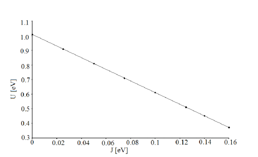
Figure 1: Set of points in $U,J$ parameter space which reproduces the commensurate resonance at 40 meV at point $\textbf{Q}_{0}=(\pi/a,\pi/a$) . The set is fitted with the linear formula $U=-3.985J+1.01$ ($U$ and $J$ are in eV). Note that $V=V_{\psi}/2-3J/4$ where $V_{\psi}=265$ meV is calculated from the gap equation by using the set of parameters given in Ref. [ARPES, ]. The maximum value of the energy gap is $\Delta=60$ meV Ref. [Delta, ].

During the second step of our approach we solved numerically the BS equations to obtain the spectrum of the collective modes $\omega(\textbf{Q})$ at the commensurate point $\textbf{Q}_{0}=(\pi/a,\pi/a)$, as well as at four incommensurate points $\pi/a(1\pm\delta,1)$ and $\pi/a(1,1\pm\delta)$. Here $\delta$ is the deviation of the collective mode position from $\textbf{Q}_{0}$. The collective-mode energy is the same at any of the four incommensurate points. Since the spin response function and the two-particle Green’s function share the same poles, we can use the 40 meV solution of the BS equations at $\textbf{Q}_{0}$ to obtain a relation between $U$ and $J$ parameters, which is presented in FIG. 1. It can be seen that the linear formula $U=-3.985J+1.01$ agrees very well with the numerical results ($U$ and $J$ are in eV). By means of the last relation we have solved the BS equations for the one of the four incommensurate 24 meV peaks observed at $(Q_{x},Q_{y})=\pi/a(1\pm\delta,1)$ and $(Q_{x},Q_{y})=\pi/a(1,1\pm\delta)$, where $\delta=0.22$ Ar . The solution provides the following interaction strengths: $J\sim 129$ meV, $V\sim 35.7$ meV and $U\sim 495$ meV.

We have tested the above values of the interaction strengths by calculating the positions of the incommensurate peaks at 32 meV. The Bethe-Salpeter equations with the above strengths provide the deviation from $\textbf{Q}_{0}$ of about $\delta=0.196$. This result is in agreement with the experimentally obtained deviation of $\delta\sim 0.19$ (see FIG. 2 in Ref. [Ar, ]). The fact that our approach is able to reproduce the 40 meV peak as well as the two peaks at 24 meV and 32 meV allows us to conclude that the commensurate resonance and incommensurate peaks have a common origin.

IV Summary and discution

The strength for $J$ should be comparable to the strength of the superexchange interactions in the underdoped antiferromagnetic insulator state of the cuprates. The superexchange interaction in cuprates has been studied by using several experimental tools, and is now known to be not strongly dependent on materials with the magnitude of $0.1-0.12$ eV. Our value of $J=0.129$ eV is larger than the accepted experimental values though some theoretical papers have predicted different magnitudes. For example, in Ref. [FJ, ] the value of $J=0.22$ eV has been predicted using standard cuprate parameters. The calculated value of the superexchange interaction in Ref. [MT, ] is about $J=0.16$ eV. The differences could be due to the fact that calculations are very sensitive to the values of the superconducting gap and the tight-binding parameters, and therefore, somewhat different tight-binding form of the mean-field electron energy could bring the calculated $J$ closer to the experimental value.

In summary, we have demonstrated that the strengths of the interactions in cuprates can be obtained if we have the angle-resolved photoemission and inelastic neutron scattering data collected on the same crystals of the high-temperature superconductor. We do not wish to repeat the theoretical arguments that were advanced against the stripes model, but our unified description of the peaks based on the $t-U-V-J$ model strongly supports the hypothesis that the commensurate resonance and the incommensurate peaks in cuprates compounds have a common origin.

References

(1)
M. Arai, T. Nishijima, Y. Endoh, T. Egami, S. Tajima, K. Tomimoto,
Y. Shiohara, M. Takahashi, A. Garrett, and S. M. Bennington, Phys.
Rev. Lett. 83, 608 (1999).
(2) H. A. Mook, P. Dai, S. M. Hayden, G. Aeppli, T. G. Perring, and
F. Dogan, Nature (London) 395, 580 (1998); P. Bourges, Y.
Sidis, H. F. Fong, L. P. Regnault, J. Bossy, A. Ivanov, and B.
Keimer, Science 288, 1234 (2000); P. Dai, H. A. Mook, R. D.
Hunt, and F. Dogan, Phys. Rev. B 63, 054525 (2001); C. D.
Batista, G. Ortiz, and A. V. Balatsky, Phys. Rev. B 64,
172508 (2001).
(3) S. A. Kivelson, I. P. Bindloss, E. Fradkin, V.
Oganesyan, J. M. Tranquada, A. Kapitulnik, and C. Howald, Rev. Mod.
Phys. 75, 1201 (2003).
(4) Q. M. Si, Y. Y. Zha, K. Levin, and J. P. Lu, Phys. Rev. B 47,
9055 (1993); D. Z. Liu, Y. Zha, and K. Levin, Phys. Rev. Lett.
75, 4130 (1995); Ying-Jer Kao, Q. Si, and K. Levin, Phys.
Rev. B 61, R11 898 (2000).
(5) S. W. Lovesey, in Theory of Thermal Neutron Scattering from
Condensed Matter (Clarendon, Oxford, 1984), Vol. 2.
(6) W.F. Brinkman, J.W. Serene, and P.W. Anderson, Phys. Rev. A 10,
2386 (1974); R. Joynt and T.M. Rice, Phys. Rev. B 38, 2345
(1988); H.Y. Kee, J. Phys.: Condens. Matter 12, 2279
(2000); D.K. Morr, P.F. Trautman, and M.J. Graf, Phys. Rev. Lett.
86, 5978 (2001); M. Yakiyama and Y. Hasegawa, Phys. Rev. B
67, 014512 (2003).
(7) C. Buhler and A. Moreo, Phys. Rev. B
59, 9882 (1999).
(8) A. P. Schnyder, A. Bill, C. Mudry, R. Gilardi, H. M. R nnow, and J.
Mesot, Phys. Rev. B 70, 214511 (2004).
(9) I. Eremin, D. K. Morr, A.V. Chubukov, K. H. Bennemann, and M. R.
Norman, Phys. Rev. Lett. 94, 147001 (2005).
(10) K. Maki, and H. Won, Phys. Rev. Leet., 72,1758
(1994)
(11) J. Brinckmann and P. A. Lee, Phys. Rev. B 65, 014502 (2001).
(12) J. Brinckmann, and P. A. Lee, Phys. Rev. Lett., 82, 2915
(1999).
(13) Jian-Xin Li, Chung-Yu Mou, and T. K. Lee, Phys. Rev. B 62, 640 (2000).
(14) Jian-Xin Li, and Chang-De Gong, Phys. Rev. B 66, 014506 (2002).
(15) H. Yamase and W. Metzner, Phys. Rev. B 73, 214517 (2006).
(16) N. Bulut and D. J. Scalapino, Phys. Rev. B
53, 5149 (1996).
(17) Z. Hao and A. V. Chubukov, Phys. Rev. B 79,
224513 (2009).
(18) W. C. Lee and A. H. MacDonald, Phys. Rev. B,
78, 174506 (2008).
(19) Z. G. Koinov, Physica C, 470, 144 (2010).
(20) R. Côté, and A. Griffin, Phys. Rev. B 48, 10404 (1993);
Wen-Cin Wu, and A. Griffin, Phys. Rev. B 51, 1190 (1995);
Phys. Rev. B 52, 7742 (1995).
(21) Z. Koinov, Phys. Rev. B 72, 085203
(2005).
(22) J. M. Tranquada, D. E. Cox, W. Kunnmann, H. Moudden, G.
Shirane, M. Suenaga, P. Zolliker, D. Vaknin, S. K. Sinha, M. S.
Alvarez, A. J. Jacobson, and D. C. Jonhston, Phys. Rev. Lett.
60, 156 (1988).
(23) I. Dimov, P. Goswami, X. Jia, and S. Chakravarty,
Phys. Rev. B 78, 134529 (2008); P. Goswami, Phys. Stat.
Sol. (B) 247, 595 (2010).
(24) M. Sutherland, D. G. Hawthorn, R. W. Hill, F. Ronning, S. Wakimoto,
H. Zhang, C. Proust, E. Boaknin, C. Lupien, L. Taillefer, R. Liang,
D. A. Bonn, W. N. Hardy, R. Gagnon, N. E. Hussey, T. Kimura, M.
Nohara, and H. Takagi, Phys. Rev. B 67, 174520 (2003).
(25) L. F. Feiner, J. H. Jefferson and R. Raimondi, Phys. Rev. B 53,
8751 (1996).
(26) Y. Mizuno, T. Tohyama, and S. Maekawa, Phys. Rev. B 58,
R14713 (1998).