Unveiling quantum entanglement degradation near a Schwarzschild black hole

Abstract

We analyze the entanglement degradation provoked by the Hawking effect in a bipartite system Alice-Rob when Rob is in the proximities of a Schwarzschild black hole while Alice is free-falling into it. We will obtain the limit in which the tools imported from the Unruh entanglement degradation phenomenon can be used properly, keeping control on the approximation. As a result, we will be able to determine the degree of entanglement as a function of the distance of Rob to the event horizon, the mass of the black hole, and the frequency of Rob’s entangled modes. By means of this analysis we will show that all the interesting phenomena occur in the vicinity of the event horizon and that the presence of event horizons do not effectively degrade the entanglement when Rob is far off the black hole. The universality of the phenomenon is presented: There are not fundamental differences for different masses when working in the natural unit system adapted to each black hole. We also discuss some aspects of the localization of Alice and Rob states. All this study is done without using the single mode approximation.

I Introduction

Relativistic quantum information is born from the combination of very different and fruitful branches of physics. Namely, general relativity, quantum field theory and quantum information theory. Its aim is to study the behavior of quantum correlations in relativistic settings. In its scope, among other topics, is the study of the behavior of quantum correlations in non-inertial settings, which has produced abundant literature Alsing and Milburn (2003); Terashima and Ueda (2004); Shi (2004); Fuentes-Schuller and Mann (2005); Alsing et al. (2006); Ball et al. (2006); Adesso et al. (2007); Brádler (2007); Ling et al. (2007); Ahn et al. (2008); Pan and Jing (2008); Alsing et al. (2004); Doukas and Hollenberg (2009); VerSteeg and Menicucci (2009); León and Martín-Martínez (2009); Adesso and Fuentes-Schuller (2009); Datta (2009); Lin and Hu (2010); Wang et al. (2010). This discipline provides novel tools for the analysis of the Unruh effect and the Hawking effect, allowing us to study the behavior of the correlations shared between non-inertial observers.

In previous works it was analyzed the entanglement degradation phenomenon produced when one of the partners of an entangled bipartite system undergoes a constant acceleration; this phenomenon, sometimes called Unruh decoherence, is strongly related to the Unruh effect. Its study revealed that there are very strong differences between fermionic and bosonic field entanglement Fuentes-Schuller and Mann (2005); Alsing et al. (2006); León and Martín-Martínez (2009); Datta (2009); Wang et al. (2010). The reason for these differences was traced back to fermionic/bosonic statistics and not to the difference between bosonic and fermionic mode population as previously thought Martín-Martínez and León (2009); Martín-Martínez and León (2010a, b). In these earlier studies some conclusions were drawn about the infinite acceleration limit, in which the situation is similar to being arbitrarily close to an event horizon of a Schwarzschild black hole.

However there are many subtleties and differences between Rindler and Schwarzschild space-times. For example Schwarzschild space-time presents a real curvature singularity while Rindler metric is nothing but the usual Minkowski metric represented in different coordinates and, therefore, has no singularities. The Rindler horizon is also of very different nature from the Schwarzschild’s event horizon. Namely, the Rindler horizon is an acceleration horizon experienced only by accelerated observers (at rest in Rindler coordinates). On the other hand, a Schwarzschild horizon is an event horizon, which affects the global causal structure of the whole space-time, independently of the observer. Also, for the Rindler space-time there are two well defined timelike Killing vectors with respect to which modes can be classified according to the criterion of being of positive or negative frequency. Contrarily, Schwarzschild space-time has only one timelike Killing vector (outside the horizon).

Therefore, to analyze the entanglement degradation produced due to the Hawking effect near a Schwarzschild black hole we must be careful, above all if we want to do a deeper study than simply taking the limit in which the Rindler acceleration parameter becomes infinite. In this paper we will show how we can use the tools coming from the study of the Unruh degradation in uniformly accelerated scenarios without restricting only to the exact infinite acceleration limit and controlling to what extent such tools are valid.

Consequently, we will be able to compute the entanglement degradation introduced by the Hawking effect as a precise function of three physical parameters, the distance of Rob to the event horizon, the mass of the black hole, and the frequency of the mode that Rob has entangled with Alice’s field state. As a result of this study we will obtain not only the explicit form of the quantum correlations as a function of the physical parameters mentioned above, but also a quantitative control on what distances from the horizon can be still analyzed using the mathematical toolbox coming from the Rindler results.

Contrarily to all the previous works in which it was carried out the single mode approximation described in Alsing et al. (2004, 2006) and of common use in the published literature, we will argue that we do not need to use such approximation to study the fundamental effects on the entanglement derived from the Hawking effect.

Our setting consists in two observers (Alice and Rob), one of them free-falling into a Schwarzschild black hole close to the horizon (Alice) and the other one standing at a small distance from the event horizon (Rob). Alice and Rob are the observers of a bipartite quantum state which is maximally entangled for the observer in free fall. The Hawking effect will introduce degradation in the state as seen by Rob, impeding all the quantum information tasks between both observers.

In this context we will analyze not only the classical and quantum correlations between Alice and Rob, but also what is the behavior of the correlations that both observers would acquire with the mode fields on the part of the space-time that is classically unaccessible due to the presence of the event horizon.

By means of this study we will show that all the interesting entanglement behavior occurs in the vicinity of the event horizon. What is more, we will argue that as the entangled partners go away from the horizon the effects on entanglement become unnoticeably small and, as a consequence, quantum information tasks in universes that contain event horizons are not jeopardized.

We will also show that the phenomenon of the Hawking degradation is universal for every Schwarzschild black hole, which is to say, it is ruled by the presence of the event horizon and is not fundamentally influenced by the specific value of the black hole parameters when the analysis is performed using natural units to the black hole. Furthermore, we will discuss the validity of the results obtained when instead of the usual plane wave basis we work in a base of wave packets, for which the states of Alice and Rob can be spatially localized.

This paper is structured as follows. In section II we show how we work without using the single mode approximation, presenting previous results about the Unruh entanglement degradation for scalar and Dirac fields. In section III we study the entanglement in a Schwarzschild space-time using the tools built for the Rindler case, detailing to what extent this approximation holds. In section IV we will present the result for the correlations between the different bipartitions in the Schwarzschild space-time scenario. In section V we show that the results obtained in the preceding sections are also valid when we consider complete sets of localized modes instead of plane waves bases. Finally, we present our conclusions in section VI.

II Rindler space-time

Along this work we are going to consider bipartite scalar and Dirac field states. We will name Alice the observer of the first part of the system and Rob the observer of the second part. In this fashion, the quantum state for the whole system is defined by the tensor product

$$\left|{\phi_{\text{A}},\phi_{\text{R}}}\right\rangle\equiv\underbrace{\left|{\phi_{\text{A}}}\right\rangle}_{\text{Alice's}}\otimes\underbrace{\left|{\phi_{\text{R}}}\right\rangle}_{\text{Rob's}}.$$ (1)

Now, while Alice is in an inertial frame, we will consider that Rob is observing the system from an accelerated frame.

A uniformly accelerated observer viewpoint is described by means of the well-known Rindler coordinates Misner et al. (1973); Takagi (1986). In order to map field states in Minkowski space-time to Rindler coordinates, two different sets of coordinates are necessary. These sets of coordinates define two causally disconnected regions in Rindler space-time. If we consider that the uniform acceleration $a$ lies on the $z$ axis, the new Rindler coordinates $(t,x,y,z)$ as a function of Minkowski coordinates $(\hat{t},\hat{x},\hat{y},\hat{z})$ are

$$a\hat{t}=e^{az}\sinh(at),\;a\hat{z}=e^{az}\cosh(at),\;\hat{x}=x,\;\hat{y}=y$$ (2)

for region I, and

$$a\hat{t}=-e^{az}\sinh(at),\;a\hat{z}=-e^{az}\cosh(at),\;\hat{x}=x,\;\hat{y}=y$$ (3)

for region IV.

Figure 1: Flat space-time conformal diagram showing Alice, Rob and AntiRob trajectories. $i^{0}$ denotes the spatial infinities, $i^{-}$, $i^{+}$ are respectively the timelike past and future infinities, $\mathscr{I}^{-}$ and $\mathscr{I}^{+}$ are the null past and future infinities respectively, and $\mathscr{H}^{\pm}$ are the Rindler horizons.

As we can see from Fig. 1, there are two more regions labeled II and III. To map them we would need to switch $\cosh\leftrightarrow\sinh$ in Eqns. (2) and (3). In these regions $t$ is a spacelike coordinate and $z$ is a timelike coordinate. However, the solutions of the Klein-Gordon/Dirac equation in such regions are not required to discuss entanglement between the inertial observer Alice and the accelerated observer Rob. This is so because Rob would be constrained to either region I or IV, having no possible access to the opposite regions as they are causally disconnected Birrell and Davies (1984); Misner et al. (1973); Takagi (1986); Fuentes-Schuller and Mann (2005); Alsing et al. (2006).

The Rindler coordinates $z,t$ go from $-\infty$ to $\infty$ independently in regions I and IV. Therefore, each region admits a separate quantization procedure with their corresponding positive and negative energy solutions of the Klein-Gordon (or Dirac) equations.

The states $\left|{1_{\hat{\omega}}}\right\rangle_{\text{M}}=a^{\dagger}_{\hat{\omega},\text{M}}\left|{0}\right\rangle_{\text{M}}$ are free massless scalar field modes, in other words, solutions of positive frequency $\hat{\omega}$ (with respect to the Minkowski timelike Killing vector $\partial_{\hat{t}}$) of the free Klein-Gordon equation:

$$\left|{1_{\hat{\omega}}}\right\rangle_{\text{M}} \equiv u_{\hat{\omega}}^{\text{M}}\propto\frac{1}{\sqrt{2{\hat{\omega}}}}e^{-i{\hat{\omega}}\hat{t}},$$

$$\left|{1_{\hat{\omega}_{1}}1_{\hat{\omega}_{2}}}\right\rangle =\left|{1_{\hat{\omega}_{1}}}\right\rangle\otimes\left|{1_{\hat{\omega}_{2}}}\right\rangle,$$ (4)

where only the time dependence has been made explicit. The label M just means that these states are expressed in the Minkowskian Fock space basis.

An accelerated observer can also define his vacuum and excited states of the field. Actually, there are two natural vacuum states associated with the positive frequency modes in regions I and IV of Rindler space-time. These are $\left|{0}\right\rangle_{\text{I}}$ and $\left|{0}\right\rangle_{\text{IV}}$, and subsequently we can define the field excitations using Rindler coordinates $(x,t)$ as

$$\left|{1_{\omega}}\right\rangle_{\text{I}} =a^{\dagger}_{\omega,\text{I}}\left|{0}\right\rangle_{\text{I}}\equiv u_{\omega}^{\text{I}}\propto\frac{1}{\sqrt{2\omega}}e^{-i\omega t},$$

$$\left|{1_{\omega}}\right\rangle_{\text{IV}} =a^{\dagger}_{\omega,\text{IV}}\left|{0}\right\rangle_{\text{IV}}\equiv u_{\omega}^{\text{IV}}\propto\frac{1}{\sqrt{2\omega}}e^{i\omega t}.$$ (5)

These modes are related by a space-time reflection and only have support in regions I and IV of the Rindler space-time respectively.

However, these Rindler modes are not independent of the Minkowskian modes. Indeed we can expand the field in terms of Minkowski modes and, independently, in terms of Rindler modes. Therefore, the Minkowskian and the Rindler set of modes are related by a change of basis León and Martín-Martínez (2009); Birrell and Davies (1984). The relationship between the Minkowski Fock basis and the two Rindler Fock bases comes through the Bogoliubov coefficients, obtained by equating the field expansion in Minkowskian modes with the field expansion in Rindler modes. In general we have that

$$u_{\hat{\omega}_{j}}^{\text{M}}=\sum_{i}\left(\alpha^{\text{I}}_{ij}u_{\omega_{i}}^{\text{I}}+\beta^{\text{IV}*}_{ij}u_{\omega_{i}}^{\text{IV}*}+\alpha^{\text{IV}}_{ij}u_{\omega_{i}}^{\text{IV}}+\beta^{\text{I}*}_{ij}u_{\omega_{i}}^{\text{I}*}\right).$$ (6)

The Bogoliubov coefficient matrices $\alpha^{R}_{ij},\beta^{R}_{ij}$ (where $R=\text{I},\text{IV}$) are given by the Klein-Gordon scalar product between both sets of modes

$$\alpha^{R}_{ij}=\left(u_{\omega_{i}}^{R},u_{\hat{\omega}_{j}}^{\text{M}}\right),\qquad\beta^{R}_{ij}=-\left(u_{\omega_{i}}^{R},u_{\hat{\omega}_{j}}^{\text{M}*}\right).$$ (7)

The relationship between modes also establishes a relationship between the Minkowski annihilation operator and the particle operators in Rindler regions I and IV:

$$a_{\hat{\omega}_{j},\text{M}}\!=\!\sum_{i}\left(\alpha^{\text{I}*}_{ij}a^{\phantom{\dagger}}_{\omega_{i},\text{I}}\!+\!\beta^{\text{IV}}_{ij}a^{\dagger}_{\omega_{i},\text{IV}}+\alpha^{\text{IV}*}_{ij}a^{\phantom{\dagger}}_{\omega_{i},\text{IV}}\!+\!\beta^{\text{I}}_{ij}a^{\dagger}_{\omega_{i},\text{I}}\right).$$ (8)

On the other hand there exist an infinite number of orthonormal bases that define the same vacuum state, namely the Minkowski vacuum $\left|{0}\right\rangle_{\text{M}}$, which can be used to expand the solutions of the Klein-Gordon equation. More explicitly, since the modes $u^{\text{M}}_{\hat{\omega}_{i}}$ have positive frequency, any complete set made out of independent linear combinations of these modes only (without including the negative frequency ones $u^{\text{M}*}_{\hat{\omega}_{i}}$) will define the same vacuum $\left|{0}\right\rangle_{\text{M}}$.

Specifically, as described in e.g. Refs. Unruh (1976); Takagi (1986); Birrell and Davies (1984) and explicitly constructed below, there exists an orthonormal basis $\{\psi_{\omega_{j}}^{\text{M}},\psi^{\prime\text{M}}_{\omega_{j}}\}$ determined by certain linear combinations of monochromatic positive frequency modes, $u^{\text{M}}_{\hat{\omega}_{i}}$

$$\psi^{\text{M}}_{\omega_{j}}=\sum_{i}C_{ij}\,u_{\hat{\omega}_{i}}^{\text{M}},\qquad\psi^{\prime\text{M}}_{\omega_{j}}=\sum_{i}C^{\prime}_{ij}\,u_{\hat{\omega}_{i}}^{\text{M}},$$ (9)

such that the Bogoliubov coefficients that relate this basis $\{\psi_{\omega_{j}}^{\text{M}},\psi^{\prime\text{M}}_{\omega_{j}}\}$ and the Rindler basis $\{u^{\text{I}}_{\omega_{i}},u^{\text{IV}}_{\omega_{i}}\}$ have the following form:

$$\hat{\alpha}^{\text{I}}_{ij} =\left(u_{\omega_{i}}^{\text{I}},\psi_{\omega_{j}}^{\text{M}}\right)=\cosh r_{\text{s},i}\,\delta_{ij},$$

$$\hat{\alpha}^{\text{IV}}_{ij} =\left(u_{\omega_{i}}^{\text{IV}},\psi_{\omega_{j}}^{\text{M}}\right)=0,$$

$$\hat{\beta}^{\text{I}}_{ij} =-\left(u_{\omega_{i}}^{\text{I}},\psi_{\omega_{j}}^{\text{M}*}\right)=0,$$

$$\hat{\beta}^{\text{IV}}_{ij} =-\left(u_{\omega_{i}}^{\text{IV}},\psi_{\omega_{j}}^{\text{M}*}\right)=-\sinh r_{\text{s},i}\,\delta_{ij},$$ (10)

and analogously for $\hat{\alpha}^{\prime\text{I,IV}}_{ij}$ and $\hat{\beta}^{\prime\text{I,IV}}_{ij}$ interchanging the labels I and IV in the formulas above. In this expressions

$$\tanh r_{\text{s},i}=\exp(-\pi{\omega_{i}}/{a}),$$ (11)

and the label s in $r_{\text{s},i}$ has been introduced to indicate that we are dealing with a scalar field. In this expression and in what follows, we will use Planck units ($\hbar=c=G=1$).

In this fashion a mode $\psi_{\omega_{j}}^{\text{M}}$ (or a mode $\psi^{\prime\text{M}}_{\omega_{j}}$) expands only in terms of mode of frequency $\omega_{j}$ in Rindler regions I and IV and for this reason we have labeled $\psi_{\omega_{j}}^{\text{M}}$ and $\psi^{\prime\text{M}}_{\omega_{j}}$ with the frequency $\omega_{j}$ of the corresponding Rindler modes. In other words, we can express a given monochromatic Rindler mode of frequency $\omega_{j}$ as a linear superposition of the single Minkowski modes $\psi_{\omega_{j}}^{\text{M}}$ and $\psi^{\prime\text{M}*}_{\omega_{j}}$ or as a polychromatic combination of the positive frequency Minkowski modes $u^{\text{M}}_{\hat{\omega}_{i}}$ and their conjugates.

Let us denote ${a_{\omega_{j}}}$ and $a_{\omega_{j}}^{\dagger}$ the annihilation and creation operators associated with modes $\psi^{\text{M}}_{\omega_{j}}$ (analogously we denote ${a^{\prime}_{\omega_{j}}}$ and $a_{\omega_{j}}^{\prime\dagger}$ the ones associated with modes $\psi^{\prime\text{M}}_{\omega_{i}}$). The Minkowski vacuum $\left|{0}\right\rangle_{\text{M}}$, which is annihilated by all the Minkowskian operators $a_{\hat{\omega}_{i},\text{M}}$, is also annihilated by all the operators $a_{\omega_{j}}$ and $a_{\omega_{j}}^{\prime}$, as we already mentioned. This comes out because any combination of Minkowski annihilation operators annihilates the Minkowskian vacuum.

Due to the Bogoliubov relationships (II) being diagonal, each annihilation operator $a_{\omega_{i}}$ can be expressed as a combination of Rindler particle operators of only one Rindler frequency $\omega_{i}$:

$$a_{\omega_{i}}=\cosh r_{\text{s},i}\,a^{\phantom{\dagger}}_{\omega_{i},\text{I}}-\sinh r_{\text{s},i}\,a^{\dagger}_{\omega_{i},\text{IV}},$$ (12)

and analogously for $a^{\prime}_{\omega_{i}}$ interchanging the labels I and IV.

An analogous procedure can be carried out for fermionic fields (e.g. Dirac fields). We can use linear combinations of monochromatic solutions of the Dirac equation $\psi^{\text{M}}_{\omega_{i},\sigma}$ and $\bar{\psi}^{\text{M}}_{\omega_{i},\sigma}$ (and their primed versions) built in the same fashion as for scalar fields:

$$\psi^{\text{M}}_{\omega_{j},\sigma}=\sum_{i}D_{ij}\,u_{\hat{\omega}_{i},\sigma}^{\text{M}}, \qquad\bar{\psi}^{\text{M}}_{\omega_{j},\sigma}=\sum_{i}E_{ij}\,v_{\hat{\omega}_{i},\sigma}^{\text{M}},$$

$$\psi^{\prime\text{M}}_{\omega_{j},\sigma}=\sum_{i}D^{\prime}_{ij}\,u_{\hat{\omega}_{i},\sigma}^{\text{M}}, \qquad\bar{\psi}^{\prime\text{M}}_{\omega_{j},\sigma}=\sum_{i}E^{\prime}_{ij}\,v_{\hat{\omega}_{i},\sigma}^{\text{M}},$$ (13)

where $u_{\hat{\omega}_{i},\sigma}^{\text{M}}$ and $v_{\hat{\omega}_{i},\sigma}^{\text{M}}$ are respectively monochromatic solutions of positive (particle) and negative (antiparticle) frequency $\pm\hat{\omega}_{i}$ of the massless Dirac equation with respect to the Minkowski Killing time. The label $\sigma$ accounts for the possible spin degree of freedom of the fermionic field.

The coefficients of these combinations are such that for the modes $\psi_{\omega_{i},\sigma}$ and $\bar{\psi}_{\omega_{i},\sigma}$ the annihilation operators are related with the Rindler ones by means of the following Bogoliubov transformations Jáuregui et al. (1991); Jianyang and Zhijian (1999); Alsing et al. (2006):

$$c_{{\omega_{i}},\sigma} = \cos{r_{\text{d},i}}\,c_{\text{I},{\omega_{i}},\sigma}-\sin r_{\text{d},i}\,d^{\dagger}_{\text{IV},{\omega_{i}},-\sigma},$$

$$d_{{\omega_{i}},\sigma}^{\dagger} = \cos{r_{\text{d},i}}\,d^{\dagger}_{\text{IV},{\omega_{i}},\sigma}+\sin r_{\text{d},i}\,c_{\text{I},{\omega_{i}},-\sigma},$$ (14)

and analogously for $c^{\prime}_{\omega_{i}}$ and $d^{\prime\dagger}_{\omega_{i}}$ interchanging the labels I and IV, where

$$\tan r_{\text{d},i}=\exp(-\pi{{\omega_{i}}}/{a}).$$ (15)

Here $c_{{\omega_{i}},\sigma}$, $d_{{\omega_{i}},\sigma}$ represent the annihilation operators of modes $\psi^{\text{M}}_{\omega_{i},\sigma}$ and $\bar{\psi}^{\text{M}}_{\omega_{i},\sigma}$ for particles and antiparticles respectively. The label d in $r_{\text{d},i}$ has been introduced to indicate Dirac field. The specific form for $\psi^{\text{M}}_{\omega_{i},\sigma}$ and $\bar{\psi}^{\text{M}}_{\omega_{i},\sigma}$ as a linear combination of monochromatic solutions of the Dirac equation can be seen, for instance, in Jáuregui et al. (1991); Jianyang and Zhijian (1999) among many other references. Notice again that, although we are denotating $a_{\omega_{i}},c_{\omega_{i},\sigma},d_{\omega_{i},\sigma}$ the operators associated with Minkowskian modes, those modes are not monochromatic, but a linear combination of monochromatic modes given by (9) and (II).

As we are going to discuss fundamental issues and not an specific experiment, there is no reason to adhere to a specific basis. Specifically, if we work in the bases (9), (II) for Minkowskian modes we do not need to carry out the single mode approximation Alsing et al. (2004, 2006) in which one single mode of Minkowski frequency $\hat{\omega}_{i}$ was expressed as a monochromatic combination of Rindler modes of the same frequency. This approximation has allowed pioneering studies of correlations with non inertial observers, but it is based on misleading assumptions on the characteristics of Rob’s detector, being partially flawed. In any case, discussing the validity of the single mode approximation is not the aim of this work. A complete discussion of the problems associated with the single mode approximation and how to overcome them is in course of completion and will be reported elsewhere et al (2010). As far as this work is concerned it is enough to say that we are not using any similar approximation.

II.1 Vacuum and first excitation for a scalar field

The Minkowski vacuum state of the field $\left|{0}\right\rangle_{\text{M}}$ is annihilated by the annihilation operators $a_{\hat{\omega}_{i},\text{M}}$ as well as by the operators $a_{\omega_{i}}$ and $a^{\prime}_{\omega_{i}}$. For the excited states of the field, we will work with the orthonormal basis $\{\psi^{\text{M}}_{\omega_{i}},\psi^{\prime\text{M}}_{\omega_{i}}\}$ defined in (9) such that

$$\left|{1_{\omega_{i}}}\right\rangle_{\text{M}}=a_{\omega_{i}}^{\dagger}\left|{0}\right\rangle_{\text{M}},\qquad|1^{\prime}_{\omega_{i}}\rangle_{\text{M}}=a^{\prime\dagger}_{\omega_{i}}\left|{0}\right\rangle_{\text{M}}$$ (16)

are solutions of the free Klein-Gordon equation which are not monochromatic, but linear superpositions of plane waves of positive frequency $\hat{\omega}_{j}$.

As shown in Takagi (1986); Birrell and Davies (1984), we can express the Minkowski vacuum state in terms of the Rindler Fock space basis, $\left|{0}\right\rangle_{\text{M}}=\bigotimes_{i}\left|{0_{\omega_{i}}}\right\rangle_{\text{M}}$, where

$$\left|{0_{\omega_{i}}}\right\rangle_{\text{M}}=\frac{1}{\cosh r_{\text{s},i}}\sum_{n=0}^{\infty}(\tanh r_{\text{s},i})^{n}\left|{n_{\omega_{i}}}\right\rangle_{\text{I}}\left|{n_{\omega_{i}}}\right\rangle_{\text{IV}}.$$ (17)

It is straightforward to check that this vacuum is, indeed, annihilated by the operators $a_{\omega_{i}}$ and $a^{\prime}_{\omega_{i}}$.

The Minkowskian one particle state $\left|{1_{\omega_{i}}}\right\rangle_{\text{M}}$ (in the basis (9)) results from applying the creation operator $a^{\dagger}_{\omega_{i}}$ to the vacuum state. We can also translate it to the Rindler basis

$$\left|{1_{\omega_{i}}}\right\rangle_{\text{M}} =\frac{1}{(\cosh r_{\text{s},i})^{2}}$$

$$\times\sum_{n=0}^{\infty}(\tanh r_{\text{s},i})^{n}\sqrt{n+1}\left|{n+1_{\omega_{i}}}\right\rangle_{\text{I}}\left|{n_{\omega_{i}}}\right\rangle_{\text{IV}}.$$ (18)

The mode $|1^{\prime}_{\omega_{i}}\rangle_{\text{M}}$ is analogous but swapping the labels I and IV.

II.2 Vacuum and first excitation for a Dirac field

For simplicity in the notation we are going to present only the construction of the modes $\psi_{\omega_{i}}^{\text{M}}$ and $\bar{\psi}_{\omega_{i}}^{\text{M}}$ in (9) since, as we will show later when we build the entangled state, they are the only ones of importance in this analysis. In any case, the construction of the primed modes for the Dirac field is analogous, but we would need to expand the notation below to include the possibility of antiparticles in Rindler region I and particles in Rindler region IV being careful with all the anticommutation subtleties typical for fermionic fields.

As for the scalar case, the vacuum state of the field $\left|{0}\right\rangle_{\text{M}}$ is annihilated by the annihilation operators $c_{\hat{\omega}_{i},\sigma,\text{M}}$ and $d_{\hat{\omega}_{i},\sigma,\text{M}}$ for all $\hat{\omega}_{i},\sigma$ as well as by the operators $c_{\omega_{i},\sigma}$ and $d_{\omega_{i},\sigma}$ for all $\omega_{i},\sigma$.

For the excited states of the field, we will work with the orthonormal basis (II) such that

$$\left|{\sigma_{\omega_{i}}}\right\rangle_{\text{M}}=c_{\omega_{i},\sigma}^{\dagger}\left|{0}\right\rangle_{\text{M}}$$ (19)

are positive frequency solutions of the free Dirac equation which are not monochromatic, but linear superpositions of plane waves of positive frequency $\hat{\omega}_{i}$.

Let us introduce some notation for the Rindler field excitations that will follow the same convention as in León and Martín-Martínez (2009); Martín-Martínez and León (2009); Martín-Martínez and León (2010a).

$$\left|{\sigma_{{\omega_{i}}}}\right\rangle_{\text{I}} =c^{\dagger}_{\text{I},{\omega_{i}},\sigma}\left|{0}\right\rangle_{\text{I}},$$

$$\left|{\sigma_{{\omega_{i}}}}\right\rangle_{\text{IV}} =d^{\dagger}_{\text{IV},{\omega_{i}},\sigma}\left|{0}\right\rangle_{\text{IV}},$$

$$\left|{p_{{\omega_{i}}}}\right\rangle_{\text{I}} =c^{\dagger}_{\text{I},{\omega_{i}},\uparrow}c^{\dagger}_{\text{I},{\omega_{i}},\downarrow}\left|{0}\right\rangle_{\text{I}}=-c^{\dagger}_{\text{I},{\omega_{i}},\downarrow}c^{\dagger}_{\text{I},{\omega_{i}},\uparrow}\left|{0}\right\rangle_{\text{I}},$$

$$\left|{p_{{\omega_{i}}}}\right\rangle_{\text{IV}} =d^{\dagger}_{\text{IV},{\omega_{i}},\uparrow}d^{\dagger}_{\text{IV},{\omega_{i}},\downarrow}\!\left|{0}\right\rangle_{\text{IV}}=-d^{\dagger}_{\text{IV},{\omega_{i}},\downarrow}d^{\dagger}_{\text{IV},{\omega_{i}},\uparrow}\!\left|{0}\right\rangle_{\text{IV}},$$ (20)

where $p_{{\omega_{i}}}$ represents the spin pair state in the mode with frequency ${\omega_{i}}$. Notice that due to the operator anticommutation relations,

$$\left|{\sigma_{{\omega_{i}}}}\right\rangle_{\text{I}}\left|{\sigma^{\prime}_{{\omega_{i}}}}\right\rangle_{\text{IV}} =c^{\dagger}_{\text{I},{{\omega_{i}}},\sigma}d^{\dagger}_{\text{IV},{\omega_{i}},\sigma^{\prime}}\left|{0}\right\rangle_{\text{I}}\left|{0}\right\rangle_{\text{IV}}$$

$$=-d^{\dagger}_{\text{IV},{{\omega_{i}}},\sigma^{\prime}}c^{\dagger}_{\text{I},{\omega_{i}},\sigma}\left|{0}\right\rangle_{\text{I}}\left|{0}\right\rangle_{\text{IV}},$$

$$d^{\dagger}_{\text{IV},{{\omega_{i}}},\sigma^{\prime}}\left|{\sigma_{{\omega_{i}}}}\right\rangle_{\text{I}}\left|{0}\right\rangle_{\text{IV}} =-\left|{\sigma_{{\omega_{i}}}}\right\rangle_{\text{I}}\left|{\sigma^{\prime}_{{\omega_{i}}}}\right\rangle_{\text{IV}}.$$ (21)

As it can be seen in León and Martín-Martínez (2009), the projection onto the unprimed sector of the basis (II) of the Minkowski vacuum state written in the Rindler basis, is as follows

$$\left|{0_{{\omega_{i}}}}\right\rangle_{\text{M}} =(\cos r_{\text{d},i})^{2}\left|{0}\right\rangle_{\text{I}}\left|{0}\right\rangle_{\text{IV}}$$

$$+\sin r_{\text{d},i}\cos r_{\text{d},i}\left(\left|{\uparrow_{{\omega_{i}}}}\right\rangle_{\text{I}}\left|{\downarrow_{{\omega_{i}}}}\right\rangle_{\text{IV}}+\left|{\downarrow_{{\omega_{i}}}}\right\rangle_{\text{I}}\left|{\uparrow_{{\omega_{i}}}}\right\rangle_{\text{IV}}\right)$$

$$+(\sin r_{\text{d},i})^{2}\left|{p_{{\omega_{i}}}}\right\rangle_{\text{I}}\left|{p_{{\omega_{i}}}}\right\rangle_{\text{IV}}.$$ (22)

It is straightforward to check that the vacuum is annihilated by $c_{{\omega_{i}},\sigma}$ and $d_{{\omega_{i}},\sigma}$ simply using (II) and applying both operators to (II.2).

The one particle state (projected onto the sector $\psi^{\text{M}}_{\omega_{i}}$ of (II)) in the Rindler basis can be readily obtained by applying the particle creation operator $c^{\dagger}_{{\omega_{i}},\sigma}$ to (II.2):

$$\left|{\uparrow_{{\omega_{i}}}}\right\rangle_{\text{M}} =\cos r_{\text{d},i}\left|{\uparrow_{{\omega_{i}}}}\right\rangle_{\text{I}}\left|{0}\right\rangle_{\text{IV}}+\sin r_{\text{d},i}\left|{p_{{\omega_{i}}}}\right\rangle_{\text{I}}\left|{\uparrow_{{\omega_{i}}}}\right\rangle_{\text{IV}},$$

$$\left|{\downarrow_{{\omega_{i}}}}\right\rangle_{\text{M}} =\cos r_{\text{d},i}\left|{\downarrow_{{\omega_{i}}}}\right\rangle_{\text{I}}\left|{0}\right\rangle_{\text{IV}}-\sin r_{\text{d},i}\left|{p_{{\omega_{i}}}}\right\rangle_{\text{I}}\left|{\downarrow_{{\omega_{i}}}}\right\rangle_{\text{IV}}.$$ (23)

II.3 Entanglement degradation due to Unruh effect

We will now summarize the results that have been obtained concerning the effects of an uniform acceleration on quantum correlations.

Let us first consider the following maximally entangled state for a scalar field:

$$\left|{\Psi}\right\rangle_{\text{s}}=\frac{1}{\sqrt{2}}\left(\left|{0}\right\rangle_{\text{A}}\left|{0}\right\rangle_{\text{R}}+\left|{1}\right\rangle_{\text{A}}\left|{1_{{\omega_{\text{R}}}}}\right\rangle_{\text{R}}\right),$$ (24)

where the label A denotes Alice’s subsystem and R denotes Rob’s subsystem. In this expression, $\left|{0}\right\rangle_{\text{A,R}}$ represents the Minkowski vacuum for Alice and Rob, $\left|{1}\right\rangle_{\text{A}}$ is an arbitrary one particle state excited from the Minkowski vacuum for Alice, and the one particle state for Rob is expressed in the basis (9) and characterized by the frequency ${\omega_{\text{R}}}$ observed by Rob.

The election of the modes $\left|{1_{\omega_{\text{R}}}}\right\rangle$ instead of $|1^{\prime}_{\omega_{\text{R}}}\rangle$ to build the maximally entangled state is not relevant since choosing the primed modes would just be equivalent to say that Rob is in region IV instead of in region I, and there is complete symmetry in all the analysis for both cases.

Since the second partner (Rob) —who observes the bipartite state (24)— is accelerated, it is convenient to map the second partition of this state into the Rindler Fock space basis, which can be computed using equations (17) and (II.1), and rewrite it in the standard language of relativistic quantum information (i.e., naming Alice to the Minkowskian observer, Rob to a hypothetic observer in Rindler’s region I and AntiRob to a hypothetic observer in Rindler Region IV):

$$\left|{\Psi}\right\rangle_{\text{s}} =\sum_{n=0}^{\infty}\frac{(\tanh r_{\text{s}})^{n}}{\sqrt{2}\cosh r_{\text{s}}}\bigg{(}\left|{0}\right\rangle_{\text{A}}\left|{n_{{\omega_{\text{R}}}}}\right\rangle_{\text{R}}\left|{n_{{\omega_{\text{R}}}}}\right\rangle_{\bar{\text{R}}}$$

$$+\left.\frac{\sqrt{n+1}}{\cosh r_{\text{s}}}\left|{1}\right\rangle_{\text{A}}\left|{n+1_{{\omega_{\text{R}}}}}\right\rangle_{\text{R}}\left|{n_{{\omega_{\text{R}}}}}\right\rangle_{\bar{\text{R}}}\right),$$ (25)

where

$$\tanh r_{\text{s}}=\exp(-\pi{\omega_{\text{R}}}/a).$$ (26)

The same can be done in the case of a Dirac field. Let us now consider the following maximally entangled state for a Dirac field in the Minkowskian basis

$$\left|{\Psi}\right\rangle_{\text{d}}=\frac{1}{\sqrt{2}}\left(\left|{0}\right\rangle_{\text{A}}\left|{0}\right\rangle_{\text{R}}+\left|{\uparrow}\right\rangle_{\text{A}}\left|{\downarrow_{\omega_{\text{R}}}}\right\rangle_{\text{R}}\right).$$ (27)

As for the bosonic case, if Rob, who observes this bipartite state, is accelerated, it is convenient to map the second partition of this state into the Rindler Fock space basis, which can be computed using Eqns. (II.2) and (II.2). The explicit form of such state can be seen in León and Martín-Martínez (2009).

Notice that we have chosen a specific maximally entangled state (27) of all the possible choices. This election has no relevance since in Martín-Martínez and León (2009) it was shown the universality of the degradation of fermionic entanglement. All fermionic maximally entangled states are equally degraded by the Unruh effect, no matter what kind of maximally entangled state is (either occupation number or spin Bell state), or even if we work with a Grassmann scalar field instead of a Dirac field.

Let us denote

$$\rho^{\text{s}}_{\text{AR}\bar{\text{R}}}=\left|{\Psi_{\text{s}}}\right\rangle\!\left\langle{\Psi_{\text{s}}}\right|,\qquad\rho^{\text{d}}_{\text{AR}\bar{\text{R}}}=\left|{\Psi_{\text{d}}}\right\rangle\!\left\langle{\Psi_{\text{d}}}\right|,$$ (28)

the tripartite density matrices for the bosonic and fermionic cases, in which we use the Minkowski basis for Alice and the Rindler basis for Rob-AntiRob. One could ask what is the physical meaning of each of these three ‘observers’. Alice represents an observer in an inertial frame. For Alice the states (24) and (27) are maximally entangled. Rob represents an accelerated observer moving in a $x=a^{-1}$ trajectory in Region I of Rindler space-time (as seen in Fig. 1) who shares a bipartite entangled state (24) or (27) with Alice. AntiRob represents an observer moving in a $x=a^{-1}$ trajectory in Region IV with access to the information to which Rob is not able to access (at least classically) due to the presence of the Rindler horizon.

In the standard Unruh entanglement degradation scenario Fuentes-Schuller and Mann (2005); León and Martín-Martínez (2009), as Rob is not able to access AntiRob part of the system we must trace over AntiRob degrees of freedom when accounting for the quantum state shared by Alice and Rob. This provokes, for instance, the observation of a thermal bath by Rob while Alice observes the Minkowski vacuum as it can be seen elsewhere Birrell and Davies (1984); Alsing et al. (2006); León and Martín-Martínez (2009). As a consequence the state becomes mixed, which causes some degree of correlation loss in the system AR as we increase the value of the acceleration $a$. In references Fuentes-Schuller and Mann (2005); Alsing et al. (2006); León and Martín-Martínez (2009); Martín-Martínez and León (2009); Datta (2009); Martín-Martínez and León (2010a, b); Wang et al. (2010) it is studied how this phenomenon affects the entanglement for different fields.

It has been also studied Alsing et al. (2006); Martín-Martínez and León (2010a, b) the correlation trade-off among the all possible bipartitions of the system, namely, Alice-Rob (AR), Alice-AntiRob $(\text{A}\bar{\text{R}})$, and Rob-AntiRob $(\text{R}\bar{\text{R}})$.

Bipartition AR is the most commonly considered in the literature. It represents the system formed by an inertial observer and the modes of the field which an accelerated observer is able to access. The second bipartition $(\text{A}\bar{\text{R}})$ represents the subsystem formed by the inertial observer Alice and the modes of the field which Rob is not able to access due to the presence of an horizon as he accelerates. Classical communication between the two partners is only allowed for the bipartitions AR and $\text{A}\bar{\text{R}}$. We will call these bipartitions ‘Classical communication allowed’ (CCA) from now on. These bipartitions are the only ones in which quantum information tasks are possible to be performed.

On the other hand, no quantum information tasks can be performed using $\text{R}\bar{\text{R}}$ correlations since classical communication between Rob and AntiRob is not allowed. Anyway, studying this bipartition is still necessary to give a complete description of the behavior of the correlation created between the space-time regions separated by the horizon.

As it is commonplace in quantum information, the partial quantum states for each bipartition are obtained by tracing over the third subsystem

$$\rho^{\text{AR}} =\operatorname{Tr}_{\bar{\text{R}}}\rho^{\text{AR}\bar{\text{R}}},$$

$$\rho^{\text{A}\bar{\text{R}}} =\operatorname{Tr}_{\text{R}}\rho^{\text{AR}\bar{\text{R}}},$$

$$\rho^{\text{R}\bar{\text{R}}} =\operatorname{Tr}_{\text{A}}\rho^{\text{AR}\bar{\text{R}}}.$$ (29)

In the cases AR and $\text{A}\bar{\text{R}}$, there are physical arguments to justify the need for this ‘tracing over’ beyond mere quantum information considerations, namely, Rob will never be able to access region IV of the space-time due to the presence of the Rindler horizon so that $\bar{\text{R}}$ (Region IV) must be traced out. Likewise, AntiRob is not able to access region I because of the horizon and hence R (Region I) must be traced out. For the subsystem ${\text{R}\bar{\text{R}}}$ this tracing over subsystem A corresponds to the standard procedure for analyzing correlations between two parts of a multipartite system. The properties of the correlations among these subsystems has been analyzed in the literature, showing a completely different behavior of quantum correlations for the CCA bipartitions depending on whether the system is fermionic or bosonic.

For fermionic fields, quantum correlations are conserved as Rob accelerates Alsing et al. (2006); Martín-Martínez and León (2009). Specifically, as entanglement in the bipartition AR is reduced, entanglement in the system $\text{A}\bar{\text{R}}$ is increased. In the limit of $a\rightarrow\infty$ some entanglement survives in all the bipartitions of the system.

For the scalar field the situation is radically different, namely, no entanglement is created in the CCA bipartitions. Moreover, the entanglement in the AR bipartition is very quickly lost as Rob accelerates, even if we artificially limit the dimension of the Hilbert space Martín-Martínez and León (2010b).

This different behavior, thought at the beginning to be a consequence of the finite dimensionality of the fermionic Hilbert space, was demonstrated to be ruled only by statistics Martín-Martínez and León (2009); Martín-Martínez and León (2010a, b), which plays a crucial role in the phenomenon of Unruh entanglement degradation. The role of statistics is so important that, for fermions, the behavior of quantum correlations has been proven to be universal Martín-Martínez and León (2009). Also, the survival of entanglement for the fermionic case, is arguably related to statistical correlations Martín-Martínez and León (2009); Martín-Martínez and León (2010a). All these aspects will be discussed in depth later on, when we present the results for the Schwarzschild black hole.

III The “Black Hole Limit”: translation Rindler-Kruskal

In this section we will study a completely new setting using the tools learned from Fuentes-Schuller and Mann (2005); Alsing et al. (2006); Martín-Martínez and León (2009); Martín-Martínez and León (2010a). We will prove in a constructive way that the entanglement degradation in the vicinity of an eternal black hole can be studied in detail with these well-known tools. By means of the construction shown below we will be able to deal with new problems such as computing entanglement loss between a free-falling observer and another one placed at fixed distance to the event horizon as a function of the distance, studying the behavior of quantum correlations in the presence of black holes. We will also show that the entanglement loss produced by an eternal black hole shows universality.

To begin this section let us work a little bit with the Schwarzschild metric

$$\text{d}s^{2}=-\left(1-\frac{2m}{r}\right)\text{d}t^{2}+\left(1-\frac{2m}{r}\right)^{-1}\text{d}r^{2}+r^{2}\text{d}\Omega^{2},$$ (30)

where $m$ is the black hole mass and $\text{d}\Omega^{2}$ is the line element in the unit sphere. Due to the symmetry of the problem we are going to restrict the analysis to the radial coordinate. To shorten notation let us write the radial part of metric as

$$\text{d}s^{2}=-f\text{d}t^{2}+f^{-1}\text{d}r^{2},$$ (31)

where $f=1-2m/r$.

We can choose to write the metric in terms of the proper time $t_{0}$ of an observer placed in $r=r_{0}$ as follows,

$$\text{d}s^{2}=-\frac{f}{f_{0}}\text{d}t_{0}^{2}+f^{-1}\text{d}r^{2},$$ (32)

where $f_{0}=1-2m/r_{0}$. The relationship between $t_{0}$ and $t$ is given by the norm of the timelike Killing vector $\xi=\partial_{t}$ in $r=r_{0}$, namely $t_{0}=\sqrt{f_{0}}\,t$.

We can now change the spatial coordinate such that the new coordinate vanishes at the Schwarzschild radius $r=R_{\text{S}}=2m$. Let us define $z$ in the following way

$$r-2m=\frac{z^{2}}{8m}\quad\Rightarrow\quad f=\frac{(\kappa z)^{2}}{1+(\kappa z)^{2}},$$ (33)

with $\kappa=1/(4m)$ being the surface gravity of the black hole. Then the metric (32) results

$$\text{d}s^{2}=-\frac{1}{f_{0}}\frac{(\kappa z)^{2}}{1+(\kappa z)^{2}}\text{d}t_{0}^{2}+\left[1+(\kappa z)^{2}\right]\text{d}z^{2}.$$ (34)

Near the event horizon ($z\approx 0$), we can expand this metric to lowest order in $z$ and approximate it by

$$\text{d}s^{2}=-\left(\frac{\kappa z}{\sqrt{f_{0}}}\right)^{2}\text{d}t_{0}^{2}+\text{d}z^{2},$$ (35)

which is a Rindler metric with acceleration parameter $\kappa/\sqrt{f_{0}}$.

On the other hand, Eq. (35) represents the metric near the event horizon in terms of the proper time of an observer placed at $r=r_{0}$. The next step is giving a physical meaning to this Rindler-like acceleration parameter. For this, we need to compute the proper acceleration of a Schwarzschild observer placed at $r=r_{0}$, which is, indeed, different from $\kappa$ (as $\kappa$ would be the acceleration of an observer arbitrarily close to the horizon as seen from a free-falling frame).

To compute $a$ for this observer as seen by himself (proper acceleration) we must start from the Schwarzschild metric. The value of the proper acceleration for an accelerated observer at arbitrary fixed position $r$ is $a=\sqrt{a_{\mu}a^{\mu}}$ where $a^{\mu}=v^{\nu}\nabla_{\nu}v^{\mu}$ is the observer 4-acceleration at such position, whereas $v^{\mu}$ is his 4-velocity.

The 4-velocity for a Schwarzschild observer in an arbitrary position $r$ is

$$v^{\mu}={\xi^{\mu}}/{|\xi|},$$ (36)

where $\xi\equiv\partial_{t}$ is the Schwarzschild timelike Killing vector. As $\xi^{\mu}=(1,0,0,0)$ in Schwarzschild coordinates, then $|\xi|=\sqrt{|g_{00}|}=\sqrt{f}$, and therefore $v^{\mu}=\xi^{\mu}/\sqrt{f}$. Thus, we can compute the acceleration 4-vector

$$a^{\mu}=v^{\nu}\nabla_{\nu}v^{\mu}=\frac{1}{|\xi|}\xi^{\nu}\nabla_{\nu}\frac{\xi^{\mu}}{|\xi|}.$$ (37)

Taking into account that $\xi^{\mu}$ is a Killing vector and, therefore, it satisfies $\nabla_{\mu}\xi_{\nu}+\nabla_{\nu}\xi_{\mu}=0$, we easily obtain

$$a_{\mu}=\frac{1}{2}\frac{\partial_{\mu}|\xi|^{2}}{|\xi|^{2}}=\frac{\partial_{\mu}f}{2f}=\frac{1}{2f}\left(0,\partial_{r}f,0,0\right).$$ (38)

Hence, since $g^{rr}=f$, the proper acceleration for this observer is

$$a=\sqrt{g^{\mu\nu}a_{\mu}a_{\nu}}=\sqrt{\frac{(\partial_{r}f)^{2}}{4f}}.$$ (39)

For an observer placed at $r=r_{0}$,

$$a_{0}=\frac{\kappa}{\sqrt{f_{0}}}(1-f_{0})^{2}.$$ (40)

We know from (33) that $1-f_{0}=[1+(\kappa z_{0})^{2}]^{-1}$. So, if the observer in $r=r_{0}$ is close to the event horizon ($r_{0}\approx R_{\text{S}}$), then, to lowest order, $1+(\kappa z_{0})^{2}\approx 1$ and

$$a\approx{\kappa}/{\sqrt{f_{0}}}.$$ (41)

Therefore, under this approximation, we can re-write (35) as

$$\text{d}s^{2}=-\left(a_{0}z\right)^{2}\text{d}t_{0}^{2}+\text{d}z^{2}.$$ (42)

This shows that the Schwarzschild metric can be approximated, in the proximities of the event horizon, by a Rindler metric whose acceleration parameter is the proper acceleration of an observer resisting in a position $r_{0}$ close enough to the event horizon.

This approximation holds if

$$\left(\frac{z_{0}}{2R_{\text{S}}}\right)^{2}\ll 1$$ (43)

or, in other words, if

$$\frac{\Delta_{0}}{R_{\text{S}}}\ll 1,$$ (44)

where $\Delta_{0}\equiv r_{0}-R_{\text{S}}$ is the distance from $r_{0}$ to the event horizon. In the limit $r_{0}\rightarrow R_{\text{S}}$ we obtain that $f_{0}\rightarrow 0$ and, from (41), $a_{0}\rightarrow\infty$. This shows rigorously that being very close to the event horizon of a Schwarzschild black hole can be very well approximated by the infinite acceleration Rindler case, as it was suggested in Fuentes-Schuller and Mann (2005); Alsing et al. (2006); Martín-Martínez and León (2009); Martín-Martínez and León (2010a). This also enables us to study what would happen with the entanglement between observers placed at different distances of the event horizon as far as the Rindler approximation holds.

Now let us identify again who is who in this new scenario. For this, we introduce the null Kruskal-Szeckeres coordinates

$$u=-\kappa^{-1}\exp[-\kappa(t-r^{*})],\quad v=\kappa^{-1}\exp[\kappa(t+r^{*})],$$ (45)

where $r^{*}=r+2m\log|1-r/2m|$. In terms of these coordinates the radial part of the Schwarzschild metric is

$$\text{d}s^{2}=\frac{-1}{2\kappa r}e^{-2\kappa r}\text{d}u\text{d}v,$$ (46)

where $r$ is implicitly defined by (45). The Penrose diagram for this maximal analytic extension is shown in Fig. 2. In this coordinates, near the horizon the metric can be written to lowest order as

$$\text{d}s^{2}=-e^{-1}\text{d}u\text{d}v$$ (47)

and $uv=-(\kappa z)^{2}$.

Figure 2: Kruskal space-time conformal diagram showing trajectories for Alice, Rob and AntiRob. $i^{0}$ denotes the spatial infinities, $i^{-}$, $i^{+}$ are respectively the timelike past and future infinities, $\mathscr{I}^{-}$ and $\mathscr{I}^{+}$ are the null past and future infinities respectively, and $\mathscr{H}^{\pm}$ are the event horizons.

Hence, there are three regions in which we can clearly define physical timelike vectors respect to which we can classify positive and negative frequencies:

• $\partial_{\hat{t}}\propto(\partial_{u}+\partial_{v})$. The parameter $\hat{t}$ for this timelike vector corresponds to the proper time of a free-falling observer close to the horizon, and it is analogous to the Minkowskian timelike Killing vector. Positive frequency modes associated to this timelike vector define a vacuum state known as the Hartle-Hawking vacuum $\left|{0}\right\rangle_{\text{H}}$, which is analogous to $\left|{0}\right\rangle_{\text{M}}$ in the Rindler case.

• $\partial_{t}\propto(u\partial_{u}-v\partial_{v})$. It is the Schwarzschild timelike Killing vector, which (when properly normalized) corresponds to an observer whose acceleration at the horizon equals the surface gravity $\kappa$ of the black hole with respect to a Minkowskian observer, or, in other words, with proper acceleration $a_{0}\approx\kappa/\sqrt{f_{0}}$ close to the horizon. The vacuum state corresponding to positive frequencies associated to this timelike Killing vector is called the Boulware vacuum $\left|{0}\right\rangle_{\text{B}}$. This state is analogous to the Rindler vacuum $\left|{0}\right\rangle_{\text{I}}$.

• There is another timelike Killing vector $-\partial_{t}$ (as in Rindler) for region IV that will allow us to define another Boulware vacuum in region IV. We will call it AntiBoulware vacuum $\left|{0}\right\rangle_{\bar{\text{B}}}$, analogous to $\left|{0}\right\rangle_{\text{IV}}$ in the Rindler case.

Now, in this scenario, $\left|{1_{\hat{\omega}}}\right\rangle_{\text{H}}=a^{\dagger}_{\hat{\omega},\text{H}}\left|{0}\right\rangle_{\text{H}}$ are free scalar field modes, in other words, solutions of positive frequency ${\hat{\omega}}$ with respect to $\partial_{\hat{t}}$ of the free Klein-Gordon equation close to the horizon

$$\left|{1_{\hat{\omega}}}\right\rangle_{\text{H}}\equiv u_{\hat{\omega}}^{\text{H}}\propto\frac{1}{\sqrt{2\hat{\omega}}}e^{-i\hat{\omega}\hat{t}}.$$ (48)

The label H just means that those states are expressed in the Hartle-Hawking Fock space basis.

An observer located at a fixed distance from the black hole can also define his own vacuum and excited states of frequency $\omega$ respect to the Killing vector $\partial_{t}$. Actually, there are two natural vacuum states associated with the positive frequency modes in both sides of the horizon these are $\left|{0}\right\rangle_{\text{B}}$ and $\left|{0}\right\rangle_{\bar{\text{B}}}$, vacua for the positive frequency modes in regions I and IV respectively (Fig. 2). Subsequently, for a scalar field, we can define the field excitations as

$$\left|{1_{\omega}}\right\rangle_{\text{B}} =a^{\dagger}_{\omega,\text{B}}\left|{0}\right\rangle_{\text{B}}\equiv u_{\omega}^{\text{B}}\propto\frac{1}{\sqrt{2\omega}}e^{-i\omega t},$$

$$\left|{1_{\omega}}\right\rangle_{\bar{\text{B}}} =a^{\dagger}_{\omega,\bar{\text{B}}}\left|{0}\right\rangle_{\bar{\text{B}}}\equiv u_{\omega}^{\bar{\text{B}}}\propto\frac{1}{\sqrt{2\omega}}e^{i\omega t}.$$ (49)

Then, the analogy between the Rindler-Minkowski and the Boulware-Hartle-Hawking states, and their relation with the standard Alice-Rob-AntiRob notation is as follows:

$$\begin{array}[]{lclcl}\left|{0}\right\rangle_{\text{R}}&\leftrightarrow&\left|{0}\right\rangle_{\text{I}}&\leftrightarrow&\left|{0}\right\rangle_{\text{B}},\\ \left|{0}\right\rangle_{\bar{\text{R}}}&\leftrightarrow&\left|{0}\right\rangle_{\text{IV}}&\leftrightarrow&\left|{0}\right\rangle_{\bar{\text{B}}},\\ \left|{0}\right\rangle_{\text{A}}&\leftrightarrow&\left|{0}\right\rangle_{\text{M}}&\leftrightarrow&\left|{0}\right\rangle_{\text{H}}.\end{array}$$ (50)

The change of basis between Hartle-Hawking modes and Boulware modes is completely analogous to the change of basis between Minkowskian modes and Rindler modes with an acceleration parameter $a_{0}=\kappa/\sqrt{f_{0}}$.

In the same fashion as for Rindler we define an orthonormal basis of Hartle-Hawking scalar field modes $\{\psi^{\text{H}}_{\omega_{j}},\psi^{\prime\text{H}}_{\omega_{j}}\}$ whose elements are superpositions of positive-frequency solutions $u_{\hat{\omega}_{i}}^{\text{H}}$ of the Klein-Gordon equation with respect to the Kruskal time $\hat{t}$ such that each element corresponds to Boulware modes of one single frequency in the Kruskal regions I and IV ($u^{\text{B}}_{\omega_{j}}$ and $u^{\bar{\text{B}}*}_{\omega_{j}}$). The same can be done for the Dirac field.

We can express the Hartle-Hawking vacuum state in terms of the Boulware Fock space basis. To do so we use what we learned from the Rindler case. Taking into account that $\left|{0}\right\rangle_{\text{H}}=\bigotimes_{i}\left|{0_{\omega_{i}}}\right\rangle_{\text{H}}$, we have that

$$\left|{0_{\omega_{i}}}\right\rangle_{\text{H}}=\frac{1}{\cosh q_{\text{s},i}}\sum_{n=0}^{\infty}(\tanh q_{\text{s},i})^{n}\left|{n_{\omega_{i}}}\right\rangle_{\text{B}}\left|{n_{\omega_{i}}}\right\rangle_{{\bar{\text{B}}}},$$ (51)

where

$$\tanh q_{\text{s},i}=\exp\left({-\pi\sqrt{f_{0}}\,\omega_{i}/{\kappa}}\right).$$ (52)

The unprimed Hartle-Hawking one particle state in the basis $\{\psi^{\text{H}}_{\omega_{j}},\psi^{\prime\text{H}}_{\omega_{j}}\}$ results from applying the corresponding creation operator to the vacuum state. We can also translate this state to the Boulware basis:

$$\left|{1_{\omega_{i}}}\right\rangle_{\text{H}} =\frac{1}{(\cosh q_{\text{s},i})^{2}}$$

$$\times\sum_{n=0}^{\infty}(\tanh q_{\text{s},i})^{n}\sqrt{n+1}\left|{n+1_{\omega_{i}}}\right\rangle_{\text{B}}\!\left|{n_{\omega_{i}}}\right\rangle_{{\bar{\text{B}}}}.$$ (53)

The Hartle-Hawking vacuum (projected onto the unprimed sector) for the Dirac case is expressed in the Boulware basis as follows

$$\left|{0_{\omega_{i}}}\right\rangle_{\text{H}} =(\cos q_{\text{d},i})^{2}\left|{0_{\omega_{i}}}\right\rangle_{\text{B}}\left|{0_{\omega_{i}}}\right\rangle_{\bar{\text{B}}}$$

$$+\sin q_{\text{d},i}\cos q_{\text{d},i}\left(\left|{\uparrow_{\omega_{i}}}\right\rangle_{{\text{B}}}\left|{\downarrow_{\omega_{i}}}\right\rangle_{\bar{\text{B}}}+\left|{\downarrow_{\omega_{i}}}\right\rangle_{\text{B}}\left|{\uparrow_{\omega_{i}}}\right\rangle_{\bar{\text{B}}}\right)$$

$$+(\sin q_{\text{d},i})^{2}\left|{p_{\omega_{i}}}\right\rangle_{\text{B}}\left|{p_{\omega_{i}}}\right\rangle_{\bar{\text{B}}},$$ (54)

whereas the projected Hartle-Hawking one particle state is expressed in the Boulware basis as

$$\left|{\uparrow_{\omega_{i}}}\right\rangle_{\text{H}} =\cos q_{\text{d},i}\left|{\uparrow_{\omega_{i}}}\right\rangle_{\text{B}}\left|{0_{\omega_{i}}}\right\rangle_{\bar{\text{B}}}+\sin q_{\text{d},i}\left|{p_{\omega_{i}}}\right\rangle_{\text{B}}\left|{\uparrow_{\omega_{i}}}\right\rangle_{\bar{\text{B}}},$$

$$\left|{\downarrow_{\omega_{i}}}\right\rangle_{\text{H}} =\cos q_{\text{d},i}\left|{\downarrow_{\omega_{i}}}\right\rangle_{\text{B}}\left|{0_{\omega_{i}}}\right\rangle_{\bar{\text{B}}}-\sin q_{\text{d},i}\left|{p_{\omega_{i}}}\right\rangle_{\text{B}}\left|{\downarrow_{\omega_{i}}}\right\rangle_{\bar{\text{B}}},$$ (55)

where this time

$$\tan q_{\text{d},i}=\exp\left(-\pi\sqrt{f_{0}}\,\omega_{i}/{\kappa}\right).$$ (56)

Thus, in this new scenario, we can consider a bipartite state analogous to the states (24) and (27) for the Rindler scenario which looks like follows, for fermions and bosons, in the basis of a free-falling observer (Alice)

$$\left|{\Psi}\right\rangle_{\text{s}} =\frac{1}{\sqrt{2}}\left(\left|{0}\right\rangle_{\text{A}}\left|{0}\right\rangle_{\text{R}}+\left|{1}\right\rangle_{\text{A}}\left|{1_{{\omega_{\text{R}}}}}\right\rangle_{\text{R}}\right),$$ (57)

$$\left|{\Psi}\right\rangle_{\text{d}} =\frac{1}{\sqrt{2}}\left(\left|{0}\right\rangle_{\text{A}}\left|{0}\right\rangle_{\text{R}}+\left|{\uparrow}\right\rangle_{\text{A}}\left|{\downarrow_{{\omega_{\text{R}}}}}\right\rangle_{\text{R}}\right).$$ (58)

This bipartite system consists in two subsystems, the first one is going to be observed by Alice, who is free-falling into the black hole and close to the event horizon, and the second one will be observed by Rob, who is near the event horizon at $r=r_{0}\approx R_{\text{S}}$. Therefore, the second partner who observes the bipartite states (57) and (58) describes them using the Boulware basis, so that it is convenient to map the second partition of these states into the Boulware Fock space basis.

Following the notation (50), to analyze the correlations among the bipartite subsystems we need to trace out the third subsystem analogously to what we did in (II.3):

$$\rho^{\text{AR}} \!\!=\! \operatorname{Tr}_{\bar{\text{R}}}\rho^{\text{AR}\bar{\text{R}}},$$

$$\rho^{\text{A}\bar{\text{R}}} \!\!=\! \operatorname{Tr}_{\text{R}}\rho^{\text{AR}\bar{\text{R}}},$$

$$\rho^{\text{R}\bar{\text{R}}} \!\!=\! \operatorname{Tr}_{\text{A}}\rho^{\text{AR}\bar{\text{R}}}.$$ (59)

It can be seen in Fig. 2 that all the information beyond the event horizon cannot be accessed by Rob. Actually, what happens beyond the horizon is determined by the information that Rob can access along with the information that AntiRob can access. In this context it makes sense to say that studying the system $\rho^{\text{R}\bar{\text{R}}}$ gives an idea of the correlations across the horizon.

IV Correlations behavior

In this section we will use the machinery we already have from the Rindler set-ups to compute the entanglement degradation as a function of the position of Rob.

First we will consider that Rob’s frequency ${\omega_{\text{R}}}$ is measured in natural units adapted to each black hole. This will show how modes of different frequencies suffer different correlation degradation. It will also show how less massive black holes produce a higher degradation than the heavier ones. Furthermore, this analysis will show the universality of the phenomenon of the Hawking entanglement degradation for Schwarzschild black holes.

After that, we will analyze the different degree of entanglement degradation experimented by an observer of fixed Boulware frequency ${\omega_{\text{R}}}$ standing at fixed distances from the event horizon for different black hole masses.

In the following subsections we will see that all the interesting behavior happens in regions in which the Rindler approximation (42) is valid. Specifically, in the plots below, the values of the distance to the horizon from which the interesting entanglement behavior appears are $\Delta_{0}\lesssim 0.05R_{\text{S}}$ in all the cases considered in this section for which, consequently, the approximation (42) holds.

IV.1 Adapted frequency

In terms of the mode frequency measured by Rob (written in units natural to the black hole, i.e. in terms of the surface gravity $\kappa$) and his position measured in Schwarzschild radii,

$$\Omega =2\pi{\omega_{\text{R}}}/\kappa=8\pi m{\omega_{\text{R}}},$$ (60)

$$R_{0} =r_{0}/R_{\text{S}}=r_{0}/(2m),$$ (61)

Eqns. (52) and (56) can be written as

$$\tanh q_{\text{s}} =\exp\left({-\frac{\Omega}{2}\sqrt{1-\frac{1}{R_{0}}}}\right),$$ (62)

$$\tan q_{\text{d}} =\exp\left({-\frac{\Omega}{2}\sqrt{1-\frac{1}{R_{0}}}}\right),$$ (63)

showing that the phenomenon of Hawking entanglement degradation presents universality, which is to say, if the frequency is measured in natural units, every Schwarzschild black hole behaves in the same way, as expected.

IV.1.1 Quantum correlations

We will use the negativity ($\mathcal{N}$) to account for the quantum correlations between the different bipartitions of the system. It is an entanglement monotone sensitive to distillable entanglement. The negativity is defined as the sum of the negative eigenvalues of the partial transpose density matrix for the system, which is defined as the transpose of only one of the subsystem q-dits in the bipartite density matrix. For a general density matrix of a bipartite system AB,

$$\rho_{\text{AB}}=\sum_{ijkl}\rho_{ijkl}\left|{i}\right\rangle_{\text{A}}\left|{j}\right\rangle_{\text{B}}\left\langle{k}\right|_{\text{A}}\left\langle{l}\right|_{\text{B}},$$ (64)

the partial transpose is defined as

$$\rho_{\text{AB}}^{\text{pT}}=\sum_{ijkl}\rho_{ijkl}\left|{i}\right\rangle_{\text{A}}\left|{l}\right\rangle_{\text{B}}\left\langle{k}\right|_{\text{A}}\left\langle{j}\right|_{\text{B}}.$$ (65)

If $\lambda_{i}$ are the eigenvalues of $\rho^{\text{pT}}_{\text{AB}}$, then

$$\mathcal{N}_{\text{AB}}=\frac{1}{2}\sum_{i}(|\lambda_{i}|-\lambda_{i})=-\sum_{\lambda_{i}<0}\lambda_{i}.$$ (66)

Hence, to compute it, we will need the partial transpose of the bipartite density matrices (III). The details associated to the diagonalization of the partial transposed density matrices for each subsystem are technically very similar to the Rindler case, and are not of much interest for the purposes of this article. All the technical aspects of such calculations can be found in Martín-Martínez and León (2010a) for Dirac and scalar fields. The results of those calculations are shown in Figs. 3 to 6. In Figs. 3 and 4 we can see the behavior of the negativity on the CCA bipartitions for different values of Rob’s frequency $\Omega$.

For the scalar field we can see that as Rob is closer to the event horizon the entanglement shared between Alice and Rob decreases. In the limit in which Rob is very close to the horizon, entanglement is completely lost. With the study performed in this work we can see the functional dependence of the entanglement with the distance to the horizon. As seen in the figures, the degradation phenomenon occurs in a narrow region very close to the event horizon. If Rob is far enough from the black hole he will not appreciate any entanglement degradation effects unless either the mass of the black hole or the frequency of the mode considered are extremely small. There must be, indeed, a minimum residual effect associated to the Hawking thermal bath experienced in the asymptotically flat region of the spacetime, far from the region in which this approximation is valid, but it is unnoticeable small. Certainly, as it will be seen in fig. 9 and the discussion below, even very close to the horizon no effective entanglement degradation occurs for physically meaningful values of mass and frequency.

If we keep the frequency measured by Rob ${\omega_{\text{R}}}$ constant, $\Omega$ will grow proportional to the black hole mass. With this in mind, Fig. 3 shows that the degradation is stronger for less massive black holes. This result is consistent with the fact that the Hawking temperature increases as the mass of the black hole goes to zero. In the next section (specifically in Fig. 9) we will show that this is not an effect of choosing natural units, when an observer is at a fixed distance of a black hole, the degradation will be higher for less massive black holes.

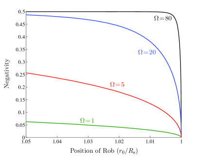
Figure 3: Scalar field: Entanglement of the system Alice-Rob as a function of the position of Rob for different values of $\Omega$. Entanglement vanishes as Rob approaches the Schwarzschild radius while no entanglement is created between Alice and AntiRob. The smaller the value of $\Omega$ the more degradation is produced by the black hole.

In any case, for the scalar field, the entanglement in the system AR is completely degraded when one of the observers is resisting very close to the event horizon of the black hole. Hence, in this scenario, no quantum information resources can be used (for instance to perform quantum teleportation or quantum computing) between a free-falling observer and an observer arbitrarily close to an event horizon. Moreover, no entanglement of any kind is created among the CCA bipartitions of the system (the ones who can classically communicate). Therefore, all useful quantum correlations between a free-falling observer and an observer at the event horizon are lost due to the Hawking effect degrading all the entanglement in the system.

For the Dirac field (Fig. 4) something very different happens. We see that correlations in the bipartition AR decrease to a certain finite limit, which means that there is entanglement survival even when Rob is asymptotically close to the event horizon. This survival is a well known phenomenon in the Rindler case Alsing et al. (2006); León and Martín-Martínez (2009). At the same time that entanglement is destroyed in the AR bipartition, entanglement is created in the complementary $\text{A}\bar{\text{R}}$ bipartition so that negativity in the CCA bipartitions fulfills a conservation law regardless of the distance to the event horizon and the mass of the black hole

$$\mathcal{N}_{\text{AR}}+\mathcal{N}_{\text{A}\bar{\text{R}}}=\frac{1}{2}.$$ (67)

The nature of this entanglement and the survival of correlations, even in the limit of positions arbitrarily close to the horizon, is discussed in Martín-Martínez and León (2010a, b) for the Rindler case. When we deal with fermionic fields there are correlations that come from the statistical fermionic nature of the field which we cannot get rid of. The hypothesis is that this entanglement, which is purely statistical, is the second quantized version of the statistical entanglement disclosed in Schliemann et al. (2001). Here we see that the same conclusions drawn in that case can be perfectly applied to the Schwarzschild black hole case.

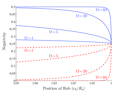
Figure 4: Dirac field: Entanglement Alice-Rob (blue solid line) and Alice-AntiRob (red dashed line). Universal conservation law for fermions is shown for different values of $\Omega$. The entanglement degradation in AR is quicker when $\Omega$ is smaller. The maximum degradation is not maximal and its value is independent of $\Omega$.

About the dependence of the entanglement degradation on the frequency of the Boulware mode, Fig. 3 shows that, for a scalar field, the loss of entanglement between a free falling observer and an observer outside but very close to the event horizon (AR) is greater for modes of lower frequency. This makes sense because, energetically speaking, it is cheaper to excite those modes and, therefore, they are more sensitive to the Hawking thermal noise. For a Dirac field (Fig. 4) we see a similar behavior, namely, lower frequencies are less protected against entanglement degradation due to Hawking effect. However, the surviving entanglement in the limit in which Rob is infinitely close to the event horizon is not sensitive to the frequency of the mode considered; remarkably, the entanglement decays up to the same finite value for all modes. This is in line with the idea that the entanglement that survives the event horizon is merely due to statistical correlations, and the only information that survives when Rob is exactly at the horizon is the fact that the field is fermionic as it is discussed in Martín-Martínez and León (2009); Martín-Martínez and León (2010a, b).

From Figs. 3 and 4 we can also conclude that all the relevant entanglement degradation phenomena is produced in the proximities of the event horizon so that the Rindler approximation that we are carrying out is valid (Eq. 44). We can also see that the degradation is small even in regions in which the approximation still holds. Therefore for longer distances from the horizon the presence of event horizons is not expected to perturb entangled systems.

In Figs. 5 and 6 we can see the behavior of the negativity on the $\text{R}\bar{\text{R}}$ bipartition for scalar and Dirac fields respectively. Here we see that quantum correlations across the horizon are created as Rob is standing closer to the event horizon. In other words, as Rob is getting closer to the event horizon the partial system $\text{R}\bar{\text{R}}$ gains quantum correlations. This result shows that, when Rob is near the horizon, the field states in both sides of the event horizon are not completely independent. Instead, they get more and more correlated. However, this $\text{R}\bar{\text{R}}$ entanglement is useless for quantum information tasks because classical communication between both sides of an event horizon is forbidden, so no quantum teleportation can be performed across the event horizon. It is well known for the Rindler case that quantum correlations are created between Rob and AntiRob Martín-Martínez and León (2010a) when the acceleration increases. Here we see the direct translation to the Kruskal scenario. The growth of those correlations encodes information about the dimension of the Fock space for each field mode Martín-Martínez and León (2010b).

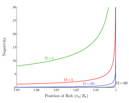
Figure 5: Scalar field: Entanglement of the system Rob-AntiRob (entanglement across the horizon) as a function of the position of Rob for different values of $\Omega$. Entanglement diverges as Rob approaches the Schwarzschild radius.

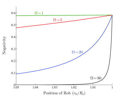
Figure 6: Dirac field: Entanglement of the system Rob-AntiRob (entanglement across the horizon) as a function of the position of Rob for different values of $\Omega$. Entanglement tends to a finite value as Rob approaches the Schwarzschild radius.

IV.1.2 Mutual information

To account for all the correlations among the different bipartitions of the system we will use the mutual information, which accounts for correlations (both quantum and classical) between two different parts of a system. For a bipartite system AB, it is defined as

$$I_{\text{AB}}=S_{\text{A}}+S_{\text{B}}-S_{\text{AB}},$$ (68)

where $S_{\text{A}}$, $S_{\text{B}}$ and $S_{\text{AB}}$ are respectively the Von Neumann entropies $S=\operatorname{Tr}\left(\rho\log_{2}\rho\right)$ for the individual subsystems A and B and for the joint system AB. To compute the mutual information for each bipartition we will need the eigenvalues of the corresponding density matrices. Again the technicalities of this analysis can be found elsewhere León and Martín-Martínez (2009); Martín-Martínez and León (2010a). The results for the CCA bipartitions are shown in Figs. 7 and 8.

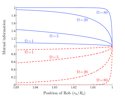
Figure 7: Scalar field: Mutual information Alice-Rob (blue solid line) and Alice-AntiRob (red dashed line). A conservation law (derived from the behavior of purely classical correlations) is shown. Mutual information AR decreases as Rob is closer to the horizon and mutual information $\text{A}\bar{\text{R}}$ grows.

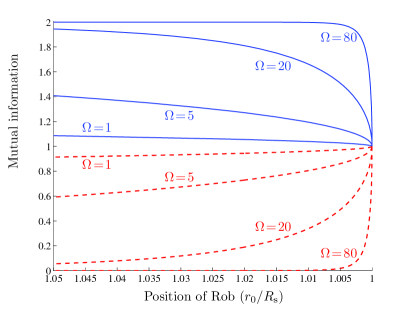
Figure 8: Dirac field: Mutual information Alice-Rob (blue solid line) and Alice-AntiRob (red dashed line). A conservation law (derived from the behavior of purely quantum correlations) is shown. Mutual information AR decreases as Rob is closer to the horizon and mutual information $\text{A}\bar{\text{R}}$ grows.

We see here that we obtain the black hole version of the mutual information universal conservation law found in previous works for the Rindler case Martín-Martínez and León (2010a). Namely, for any distance to the horizon or black hole mass it is fulfilled that

$$I_{\text{AR}}+I_{\text{A}\bar{\text{R}}}=2.$$ (69)

Although, as we can see comparing Figs. 7 and 8, the behavior of the mutual information is very similar for both fermions and bosons, the origin of this conservation law near the event horizon is completely different.

For scalar fields this conservation near the horizon responds to a conservation of classical correlations only. This can be deduced from Fig. 3 which shows that quantum correlations drop very quickly as the distance of Rob to the horizon decreases and, consequently, the only correlations left must be classical. However, the conservation of classical correlations in the CCA bipartitions has to do with the infiniteness of the dimension of the Hilbert space, as it is shown in Martín-Martínez and León (2010b). If the dimension of a bosonic field is limited to a finite value, classical correlations also drop as Rob is closer to the horizon (as quantum correlations do).

On the other hand, a Dirac field has a built-in dimensional limit for the Hilbert space of each mode imposed by Pauli exclusion principle. Although previous works demonstrated that this limit in the dimension has nothing to do with the behavior of quantum correlations Martín-Martínez and León (2009); Martín-Martínez and León (2010a), it does limit the creation of classical correlations. Analogously to what is discussed in Martín-Martínez and León (2010b), the origin for the conservation law (69) in the fermionic case is a direct consequence of the quantum correlations conservation law (67).

The conclusion is that, although (69) is universal for scalar and Dirac fields in the proximity of an eternal black hole, its origin is completely different. For scalar fields it responds to a conservation of classical correlations while for Dirac fields it is reflecting the quantum correlations conservation (67).

Mutual information for the $\text{R}\bar{\text{R}}$ bipartition does not add any new result as it inherits the quantum correlations behavior showed in Figs. 3 and 4.

IV.2 Entanglement degradation dependence on the black hole mass

In this section we will analyze the entanglement degradation for an observer with the same characteristics in the presence of different black holes. To do so we are going to use the full dimensional quantities ${\omega_{\text{R}}}$ and $\Delta_{0}$.

We will consider that Rob’s mode frequency is ${\omega_{\text{R}}}=1.5$ Mhz, and he is standing at a distance $\Delta_{0}=1$ cm and $\Delta_{0}=10$ cm from the event horizon of black holes with different masses, while he shares an entangled state (57) or (58) with a free-falling observer Alice.

The quantum correlations that Rob and Alice share are shown in Figs. 9 and 10 for scalar and Dirac fields, respectively. From these figures we see that for a really close distance from the event horizon, only small black holes would produce significant entanglement degradation. Actually, the degradation decreases very quickly as the black hole mass is increased.

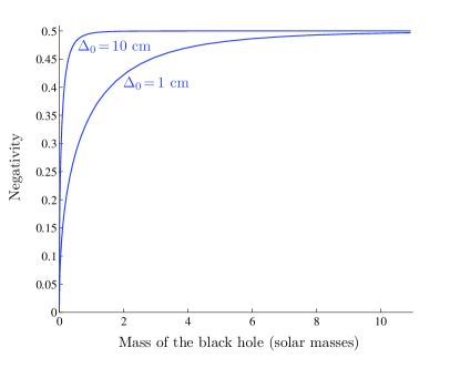
Figure 9: Scalar field: Entanglement Alice-Rob when Rob stands at a distance of 1 cm and 10 cm from the event horizon for a fixed frequency ${\omega_{\text{R}}}=1.5$ Mhz as a function of the black hole mass. Notice that, for these values of $\Delta_{0}$, the approximation holds perfectly for any mass $m>10^{-5}$ solar masses.

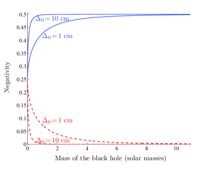
Figure 10: Dirac field: Entanglement AR (blue continuous line) and $\text{A}\bar{\text{R}}$ (red dashed line) when Rob stands at a distance of 1 cm and 10 cm from the event horizon for a fixed frequency ${\omega_{\text{R}}}=1.5$ Mhz as a function of the black hole mass. Notice that, for these values of $\Delta_{0}$, the approximation holds perfectly for any mass $m>10^{-5}$ solar masses.

Furthermore, we can see that the effects on the entanglement decrease very quickly as the distance to the event horizon is increased. This shows that quantum information tasks can be safely performed in universes that present event horizons since only in the closest vicinity of the less massive black holes the Hawking effect impedes the application of quantum information protocols.

V Localization of the states

Along this work we have used a plane-wave-like basis to express the quantum state of the field for the inertial an accelerated observers. These plane wave modes are completely delocalized, and therefore, they are not the most natural election of modes if we want to think of the observers Alice and Rob spatially localized to some degree.

However, a very similar analysis to the one carried out in sections II and III can be performed using a complete set of wave packet modes for both the Minkowski and Rindler solutions of the wave equation. These modes can be spatially localized and provide a clearer physical interpretation for Alice and Rob, which will eventually have to carry out measurements on the field. The way to build these wave packet modes can be found elsewhere Hawking (1975); Takagi (1986); Audretsch and Müller (1994).

The elements of this basis are defined as a function of the plane wave modes (II) as

$$u^{\text{M}}_{\hat{\omega},l}=\frac{1}{\sqrt{\epsilon}}\int_{\hat{\omega}}^{\hat{\omega}+\epsilon}d\nu\,e^{-i\nu l}u^{\text{M}}_{\nu},$$ (70)

where $\hat{\omega}$ and $l$ label each wave packet.

We can define creation an annihilation operators associated to these wavepackets $a_{\hat{\omega},l,\text{M}}$, $a_{\hat{\omega},l,\text{M}}^{\dagger}$ such that $a_{\hat{\omega},l,\text{M}}$ annihilates the Minkowski vacuum and $a_{\hat{\omega},l,\text{M}}^{\dagger}\left|{0}\right\rangle_{\text{M}}=\left|{1_{\hat{\omega},l}}\right\rangle_{\text{M}}$ represents a wavepacket peaked for a frequency $\hat{\omega}$ and whose spatial localization can be associated to the maximum of $u^{\text{M}}_{\omega,l}$ as a function of $\hat{x}$ and $\hat{t}$.

A similar analysis can be done for the Rindler basis

$$u^{\text{I}}_{\omega,l^{\prime}} =\frac{1}{\sqrt{\epsilon}}\int_{\omega}^{\omega+\epsilon}d\nu\,e^{-i\nu l^{\prime}}u^{\text{I}}_{\nu},$$

$$u^{\text{IV}}_{\omega,l^{\prime}} =\frac{1}{\sqrt{\epsilon}}\int_{\omega}^{\omega+\epsilon}d\nu\,e^{-i\nu l^{\prime}}u^{\text{IV}}_{\nu},$$ (71)

$\omega$ and $l^{\prime}$ label each wave packet. We can define creation an annihilation operators associated to these wavepackets $a_{\omega,l^{\prime},R}$, $a_{\omega,l^{\prime},R}^{\dagger}$ (where $R=\text{I},\text{IV}$) such that $a_{\omega,l^{\prime},R}$ annihilates the region Rindler region $R$ vacuum and $a_{\omega,l^{\prime},R}^{\dagger}\left|{0}\right\rangle_{R}=\left|{1_{\omega,l^{\prime}}}\right\rangle_{R}$ represents a wavepacket peaked for a Rindler frequency $\omega$ and whose spatial localization can be associated to the maximum of $u^{R}_{\omega,l^{\prime}}$ as a function of $x$ and $t$.

We can compute then the Bogoliuvob transformation between the Minkowski wavepackets and the Rindler wavepackets Audretsch and Müller (1994)

$$a_{\hat{\omega},l,\text{M}}=\alpha^{\text{I}*}_{\omega,l^{\prime},\hat{\omega},l}\,a^{\phantom{\dagger}}_{\omega,l^{\prime},\text{I}}+\beta^{\text{IV}}_{\omega,l^{\prime},\hat{\omega},l}\,a^{\dagger}_{\omega,l^{\prime},\text{IV}}.$$ (72)

Where the Bogoliuvob coefficients are computed in the same fashion as for the plane wave case

$$\alpha^{\text{I}}_{\omega,l^{\prime},\hat{\omega},l}=\left(u^{\text{I}}_{\omega,l^{\prime}},u^{\text{M}}_{\hat{\omega},l}\right),\quad\beta^{\text{IV}}_{\omega,l^{\prime},\hat{\omega},l}=-\left(u^{\text{IV}}_{\omega,l^{\prime}},u^{\text{M}*}_{\hat{\omega},l}\right).$$ (73)

It is shown in Audretsch and Müller (1994) that, apart from an irrelevant phase factor, the Bogoliuvob coefficients are related with (II) as follows

$$\alpha^{\text{I}}_{\omega,l^{\prime},\hat{\omega},l} =\hat{\alpha}^{\text{I}}_{ij}\,\mathcal{G}_{\alpha}(\hat{\omega},l,\omega,l^{\prime}),$$

$$\beta^{\text{I}}_{\omega,l^{\prime},\hat{\omega},l} =\hat{\beta}^{\text{IV}}_{ij}\,\mathcal{G}_{\beta}(\hat{\omega},l,\omega,l^{\prime}).$$ (74)

It is shown in Audretsch and Müller (1994) that $\mathcal{G}_{\alpha}(\hat{\omega},l,\omega,l^{\prime})\approx\delta_{\omega\omega_{\alpha}}\delta_{ll_{\alpha}}$ and $\mathcal{G}_{\beta}(\hat{\omega},l,\omega,l^{\prime})\approx\delta_{\omega\omega_{\beta}}\delta_{ll_{\beta}}$, where $l_{\alpha}=l_{\alpha}(l^{\prime})$ and $\omega_{\alpha}=\omega_{\alpha}(\omega,l^{\prime})$.

The key feature of this transformations is that they have again a diagonal form. As it can be read from (V), a Minkowski wavepacket $\left|{1_{\omega,l^{\prime}}}\right\rangle_{\text{M}}$ is connected with a pair of Rindler wavepackets in regions I and IV. Moreover, the functional form of the dependence of this coefficients with the acceleration is effectively the same. This analysis made for the Rindler and Minkowskian modes can be straightforwardly translated to the Boulware and Hartle-Hawking modes. A completely analogous analysis can be done for the fermionic case.

Consequently all the conclusions extracted in this article for delocalised modes are also valid for the localized modes defined above.

VI Conclusions

We have analyzed the entanglement degradation produced in the vicinity of a Schwarzschild black hole.

With this aim, we have carried out a detailed study of the Schwarzschild metric in the proximity of the horizon, showing how we can adapt the tools developed in the study of the entanglement degradation for uniformly accelerated observers Fuentes-Schuller and Mann (2005); Alsing et al. (2006); León and Martín-Martínez (2009); Martín-Martínez and León (2010a) to the black hole case. In particular, we have shown that, regarding entanglement degradation effects, the Rindler limit of infinite acceleration reproduces a black hole scenario in which Rob is arbitrarily close to the event horizon. More importantly, we have shown the fine structure of this limit, making explicit the dependence of the entanglement degradation phenomena on the distance to the horizon, the mass of the black hole, and the Boulware frequency ${\omega_{\text{R}}}$ of the entangled mode under consideration, while keeping control of the approximation to make sure that the toolbox developed for the Rindler case can be still rigorously used here.

By means of this analysis we have seen that all the interesting entanglement degradation phenomena due to the Hawking effect are produced very close to the event horizon of the Schwarzschild black hole. The entanglement degradation introduced by the Hawking effect becomes quickly negligible as Rob is further away from the event horizon. In other words, quantum information tasks done far away from event horizons are not perturbed by the existence of such horizons.

We have also shown that for a fixed Rob’s mode frequency and at a fixed distance from the event horizon the entanglement degradation is greater for less massive black holes. This is consistent with the fact that the Hawking temperature is higher for less massive black holes. Furthermore, the Hawking entanglement degradation is a universal phenomenon in the sense that the degradation depends only on Rob’s frequency and his distance to the horizon in units natural to the black hole (namely, the surface gravity for frequencies and the Schwarzschild radius for distances). In these units, there is no extra dependence on the black hole mass, as expected.

We have been able to adapt all the conclusions drawn for the Rindler case to the Schwarzschild scenario. In particular, we have seen that bosonic and fermionic entanglement behave in a very different way in the proximity of a black hole. As it was known for the Rindler case Martín-Martínez and León (2010a), entanglement on the CCA bipartitions is completely lost for the scalar field while there is a quantum correlation conservation law for the Dirac field.

In Martín-Martínez and León (2009) it was shown that for two different kinds of fermionic fields (Dirac fields or Grassmann scalars) and also for different maximally entangled states (occupation number or spin Bell states) the entanglement in the CCA bipartitions behaves exactly the same way. This fact was used to argue that it is statistics and not dimensionality that determines the behavior of correlations in the CCA bipartitions in the case of uniformly accelerated observers. This study proves that this argument is also valid for Schwarzschild black holes, not only in the limit in which Rob is on the event horizon, but in the whole region in which the interesting entanglement degradation phenomena are produced. Therefore, the universal fermionic entanglement behavior is also manifest in the presence of a black hole.

For the Schwarzschild case, there also appears the universal mutual information conservation law found for both scalar and Dirac fields in the Rindler case Martín-Martínez and León (2010a). In the fermionic case, it is due to a conservation of quantum correlations while, for bosons, it only reflects the conservation of classical correlations that happens in the case of infinite dimensional Hilbert spaces for each mode.

Moreover, as Rob is getting closer to the event horizon, quantum correlations between modes on both sides of the event horizon are created, namely the correlations between field modes in region I and IV of the Kruskal space-time grow up to a value determined by the dimension of the Hilbert space of each mode, which is finite for the fermionic case and infinite for the scalar field.

As discussed previously for the Rindler scenario Martín-Martínez and León (2009); Martín-Martínez and León (2010a, b), and unveiled here for the Schwarzschild black hole case, under the hypothesis that the fermionic entanglement which survives the event horizon is of statistic nature as in Schliemann et al. (2001), it would not contain any useful information. Therefore if an entangled pair is created close to the event horizon (for instance particle/antiparticle creation) and one of the subsystems falls into the black hole while the other resists close to the horizon, no other entanglement except for the mere statistical would survive the degradation provoked by the Hawking effect.

The problem of the localization of the Rindler and Minkowski modes has also been analyzed, showing that the results obtained here can be extrapolated to the case in which we consider a complete set of localized wave packets as a basis of the Fock space for the inertial and accelerated observers.

The scenario that we have discussed here is that of a static eternal black hole in which no dynamics is present. The analysis of entanglement degradation due to the dynamical creation of an event horizon in a gravitational collapse scenario is under current development and will be reported elsewhere.

VII Acknowledgments

The authors would like to thank Bei-Lok Hu, Ivette Fuentes, Robert Mann and Paul Alsing for the helpful discussions during the International Workshop on Relativisitc Quantum Information (RQI-N 2010).

The authors also thank Jorma Louko and Carlos Barceló for their helpful comments and observations.

This work was partially supported by the Spanish MICINN Projects FIS2008-05705/FIS and FIS2008-06078-C03-03, the CAM research consortium QUITEMAD S2009/ESP-1594, and the Consolider-Ingenio 2010 Program CPAN (CSD2007-00042). E. M-M was partially supported by a CSIC JAE-PREDOC2007 Grant.

References

- Alsing and Milburn (2003) P. M. Alsing and G. J. Milburn, Phys. Rev. Lett. 91, 180404 (2003).
- Terashima and Ueda (2004) H. Terashima and M. Ueda, Phys. Rev. A 69, 032113 (2004).
- Shi (2004) Y. Shi, Phys. Rev. D 70, 105001 (2004).
- Fuentes-Schuller and Mann (2005) I. Fuentes-Schuller and R. B. Mann, Phys. Rev. Lett. 95, 120404 (2005).
- Alsing et al. (2006) P. M. Alsing, I. Fuentes-Schuller, R. B. Mann, and T. E. Tessier, Phys. Rev. A 74, 032326 (2006).
- Ball et al. (2006) J. L. Ball, I. Fuentes-Schuller, and F. P. Schuller, Phys. Lett. A 359, 550 (2006).
- Adesso et al. (2007) G. Adesso, I. Fuentes-Schuller, and M. Ericsson, Phys. Rev. A 76, 062112 (2007).
- Brádler (2007) K. Brádler, Phys. Rev. A 75, 022311 (2007).
- Ling et al. (2007) Y. Ling, S. He, W. Qiu, and H. Zhang, J. of Phys. A 40, 9025 (2007).
- Ahn et al. (2008) D. Ahn, Y. Moon, R. Mann, and I. Fuentes-Schuller, J. High Energy Phys. 2008, 062 (2008).
- Pan and Jing (2008) Q. Pan and J. Jing, Phys. Rev. D 78, 065015 (2008).
- Alsing et al. (2004) P. M. Alsing, D. McMahon, and G. J. Milburn, J. Opt. B: Quantum Semiclass. Opt. 6, S834 (2004).
- Doukas and Hollenberg (2009) J. Doukas and L. C. L. Hollenberg, Phys. Rev. A 79, 052109 (2009).
- VerSteeg and Menicucci (2009) G. VerSteeg and N. C. Menicucci, Phys. Rev. D 79, 044027 (2009).
- León and Martín-Martínez (2009) J. León and E. Martín-Martínez, Phys. Rev. A 80, 012314 (2009).
- Adesso and Fuentes-Schuller (2009) G. Adesso and I. Fuentes-Schuller, Quant. Inf. Comput. 76, 0657 (2009).
- Datta (2009) A. Datta, Phys. Rev. A 80, 052304 (2009).
- Lin and Hu (2010) S.-Y. Lin and B. L. Hu, Phys. Rev. D 81, 045019 (2010).
- Wang et al. (2010) J. Wang, J. Deng, and J. Jing, Phys. Rev. A 81, 052120 (2010).
- Martín-Martínez and León (2009) E. Martín-Martínez and J. León, Phys. Rev. A 80, 042318 (2009).
- Martín-Martínez and León (2010a) E. Martín-Martínez and J. León, Phys. Rev. A 81, 032320 (2010a).
- Martín-Martínez and León (2010b) E. Martín-Martínez and J. León, Phys. Rev. A 81, 052305 (2010b).
- Misner et al. (1973) C. W. Misner, K. S. Thorne, and J. A. Wheeler, Gravitation (W. H. Freeman, 1973).
- Takagi (1986) S. Takagi, Prog. Theor. Phys. Suppl. 88, 1 (1986).
- Birrell and Davies (1984) N. D. Birrell and P. C. W. Davies, Quantum Fields in Curved Space (Cambridge University Press, 1984).
- Unruh (1976) W. G. Unruh, Phys. Rev. D 14, 870 (1976).
- Jáuregui et al. (1991) R. Jáuregui, M. Torres, and S. Hacyan, Phys. Rev. D 43, 3979 (1991).
- Jianyang and Zhijian (1999) Z. Jianyang and L. Zhijian, Int. Jour. Theor. Phys 38, 575 (1999).
- et al (2010) D. B. et al, in preparation (2010).
- Schliemann et al. (2001) J. Schliemann, J. I. Cirac, M. Kuś, M. Lewenstein, and D. Loss, Phys. Rev. A 64, 022303 (2001).
- Hawking (1975) S. W. Hawking, Commun. Math. Phys. 43, 199 (1975).
- Audretsch and Müller (1994) J. Audretsch and R. Müller, Phys. Rev. D 49, 4056 (1994).