Interaction strengths in cuprates from the inelastic neutron-scattering measurements

Abstract

The $t-U-V-J$ model is used to describe the positions of the experimental peaks associated with commensurate and incommensurate structure of the magnetic susceptibility probed by neutron scattering in cuprate compounds. Assuming that the tight-binding form of the mean-field electron energy and the maximum gap can be obtained by fitting the angle-resolved photoemission spectroscopy (ARPES) data, we have determined the strengths of the on-site repulsive interaction $U$, the spin-independent attractive interaction $V$ and the spin-dependent antiferromagnetic interaction $J$ from the positions of the commensurate and incommensurate peaks.

Introduction. It is evident from many experimentsNSS ; Bi ; Ar that the spin excitation spectrum in the superconducting state of cuprate compounds for low temperature and low energy consists of incommensurate (IC) magnetic peaks at the quartet of wavevectors $\textbf{Q}_{\delta}=(\pi(1\pm\delta),\pi(1\pm\delta))$ where $\delta$ represents the degree of incommensurability (the lattice parameter $a=1$ and $\hbar=1$ are set to unity, $\textbf{Q}_{\delta}$ corresponds to $(0.5(1\pm\delta),0.5(1\pm\delta))$ in reciprocal lattice units, r.l.u., and the total number of sites is $N$). $\delta$ decreases with increasing the energy transfer $\omega$ and vanishes at energy $\omega_{res}$. This commensurate peak is called a magnetic resonance peak and it is centered at the antiferromagnetic wave vector $\textbf{Q}_{AF}=(\pi,\pi)$. It was suggestedPlas ; Plas1 ; HC that the existence of the resonance peak in Bi2212 samples is related to two strong interactions: an on-site repulsion $U$ which drives the system close to an antiferromagnetic instability, and a short-range antiferromagnetic interaction $J$ related to the fact that cuprates are oxides of copper doped with various other atoms (doped antiferromagnetic Mott insulators). Since d-wave superconductivity on the cuprate square lattice does not rule out the existence of a spin-independent attractive interaction, we naturally arrive at the idea that the $t-U-V-J$ model could be a possible theoretical scenario which fits together three major parts of the high-$T_{c}$ superconductivity puzzle of the cuprate compounds: (i) it describes the opening of a d-wave pairing gap, (ii) it is consistent with the fact that the basic pairing mechanism arises from the antiferromagnetic exchange correlations, and (iii) it takes into account the charge fluctuations associated with double occupancy of a site which play an essential role in doped systems.

In the one-layer approximation, the Hamiltonian of the two-dimensional $t-J-U-V$ model is:

$$\widehat{H}=-\sum_{i,j,\sigma}t_{ij}\psi^{\dagger}_{i,\sigma}\psi_{j,\sigma}-\mu\sum_{i,\sigma}\widehat{n}_{i,\sigma}+U\sum_{i}\widehat{n}_{i,\uparrow}\widehat{n}_{i,\downarrow}$$

$$-V\sum_{<i,j>\sigma\sigma^{\prime}}\widehat{n}_{i,\sigma}\widehat{n}_{j,\sigma^{\prime}}+J\sum_{<i,j>}\overrightarrow{\textbf{S}}_{i}\textbf{.}\overrightarrow{\textbf{S}}_{j},$$ (1)

where $\mu$ is the chemical potential. The Fermi operator $\psi^{\dagger}_{i,\sigma}$ ($\psi_{i,\sigma}$) creates (destroys) a fermion on the lattice site $i$ with spin projection $\sigma=\uparrow,\downarrow$ along a specified direction, and $\widehat{n}_{i,\sigma}=\psi^{\dagger}_{i,\sigma}\psi_{i,\sigma}$ is the density operator on site $i$ with a position vector $\textbf{r}_{i}$. The symbol $\sum_{<ij>}$ means sum over nearest-neighbor sites. The spin operator is defined by $\overrightarrow{\textbf{S}}_{i}=\psi^{\dagger}_{i,\sigma}\overrightarrow{\sigma}_{\sigma\sigma^{\prime}}\psi_{i,\sigma^{\prime}}/2$, where $\overrightarrow{\sigma}$ is the vector formed by the Pauli spin matrices $(\sigma_{x},\sigma_{y},\sigma_{z})$. The terms in (1) represent the hopping of electrons between sites of the lattice, their on-site repulsive interaction ($U>0$), the attractive interaction between electrons on different sites of the lattice ($V>0$) and the spin-dependent Heisenberg near-neighbor interactions, respectively.

The gap equation in the case of d-wave pairing

$$1=\frac{V_{\psi}}{2}\int^{\pi}_{-\pi}\int^{\pi}_{-\pi}\frac{d\textbf{k}}{(2\pi)^{2}}\frac{d^{2}_{\textbf{k}}}{\sqrt{\overline{\varepsilon}^{2}_{\textbf{k}}+\Delta^{2}_{\textbf{k}}}},$$ (2)

where $V_{\psi}=2V+3J/2$, $E(\textbf{k})=\sqrt{\overline{\varepsilon}^{2}_{\textbf{k}}+\Delta^{2}_{\textbf{k}}}$, and $\Delta_{\textbf{k}}=\Delta(\cos k_{x}-\cos k_{y})/2$ provides a relationship between the strengths of the $V$ and $J$ interactions. The mean-field electron energy $\overline{\varepsilon}_{\textbf{k}}$ has a tight-binding form $\overline{\varepsilon}_{\textbf{k}}=t_{1}\left(\cos k_{x}+\cos k_{y}\right)/2+t_{2}\cos k_{x}\cos k_{y}+t_{3}(\cos 2k_{x}+\cos 2k_{y})/2+t_{4}(\cos 2k_{x}\cos k_{y}+\cos 2k_{y}\cos k_{x})/2+t_{5}\cos 2k_{x}\cos 2k_{y}-\mu$ obtained by fitting the ARPES data with a chemical potential $\mu$ and hopping amplitudes $t_{i}$ for first to fifth nearest neighbors on a square lattice. Since the spin susceptibility and the two-particle Green’s function share common poles, we can adjust the parameters $U,V$ and $J$ in such a way that the resonance peak $\omega_{res}$ is a solution of the Bethe-Salpeter (BS) equations for the spin collective mode of the Hamiltonian (1) at a wave vector $\textbf{Q}_{AF}$. The observed IC peaks are also poles of the spin susceptibility (or solutions of the BS equations), and therefore, we can use any of the IC resonances to obtain the exact strengths of the interactions. The calculated strengths could be tested using the positions of the other IC peaks observed on the same sample but at different transfer energy.

Bethe-Salpeter equations for the collective modes. Thought the method for solving the BS equation is not new,KN we tread the subject in detail for the sake of completeness. The antiferromagnetic spin-dependent interaction $J\sum_{<i,j>}\overrightarrow{\textbf{S}}_{i}\textbf{.}\overrightarrow{\textbf{S}}_{j}=J_{1}+J_{2}$ consists of two terms: $J_{1}=\frac{J}{4}\sum_{<i,j>}[\widehat{n}_{i,\uparrow}\widehat{n}_{j,\uparrow}+\widehat{n}_{i,\downarrow}\widehat{n}_{j,\downarrow}-\widehat{n}_{i,\uparrow}\widehat{n}_{j,\downarrow}-\widehat{n}_{i,\downarrow}\widehat{n}_{j,\uparrow}]$ and $J_{2}=\frac{J}{2}\sum_{<i,j>}\left[\psi^{\dagger}_{i,\uparrow}\psi_{i,\downarrow}\psi^{\dagger}_{j,\downarrow}\psi_{j,\uparrow}+\psi^{\dagger}_{i,\downarrow}\psi_{i,\uparrow}\psi^{\dagger}_{j,\uparrow}\psi_{j,\downarrow}\right]$. The interaction described by the $J_{2}$ term does not allow us to use two-component Nambu fermion fields, and therefore, we introduce four-component Nambu fermion fields $\widehat{\overline{\psi}}(y)=\left(\psi^{\dagger}_{\uparrow}(y)\psi^{\dagger}_{\downarrow}(y)\psi_{\uparrow}(y)\psi_{\downarrow}(y)\right)$ and $\widehat{\psi}(x)=\left(\psi^{\dagger}_{\uparrow}(x)\psi^{\dagger}_{\downarrow}(x)\psi_{\uparrow}(x)\psi_{\downarrow}(x)\right)^{T}$, where $x$ and $y$ are composite variables and the field operators obey anticommutation relations. The ”hat” symbol over any quantity $\widehat{O}$ means that this quantity is a matrix.

The interaction part of the extended Hubbard Hamiltonian is quartic in the Grassmann fermion fields so the functional integrals cannot be evaluated exactly. However, we can transform the quartic terms to a quadratic form by applying the Hubbard-Stratonovich transformation for the electron operators:ZK1

$$\begin{split}&\int DAe^{\left[\frac{1}{2}A_{\alpha}(z)D_{\alpha\beta}^{(0)-1}(z,z^{\prime})A_{\beta}(z)+\widehat{\overline{\psi}}(y)\widehat{\Gamma}^{(0)}_{\alpha}(y;x|z)\widehat{\psi}(x)A_{\alpha}(z)\right]}\\ &=e^{-\frac{1}{2}\widehat{\overline{\psi}}(y)\widehat{\Gamma}^{(0)}_{\alpha}(y;x|z)\widehat{\psi}(x)D_{\alpha\beta}^{(0)}(z,z^{\prime})\widehat{\overline{\psi}}(y^{\prime})\widehat{\Gamma}^{(0)}_{\beta}(y^{\prime};x^{\prime}|z^{\prime})\widehat{\psi}(x^{\prime})}.\end{split}$$ (3)

The last equation is used to define the $4\times 4$ matrices $\widehat{D}_{\alpha\beta}^{(0)}$ and $\widehat{\Gamma}^{(0)}_{\alpha}$ ($\alpha,\beta=1,2,3,4$). Their Fourier transforms, written in terms of the Pauli $\sigma_{i}$, Dirac $\gamma^{0}$ and alphaY; B matrices, are as follows: $\widehat{D}^{(0)}=\left(\begin{array}[]{cc}\widehat{D}_{1}&0\\ 0&\widehat{D}_{2}\end{array}\right)$, $\widehat{\Gamma}_{1,2}^{(0)}=(\gamma^{0}\pm\alpha_{z})/2$ and $\widehat{\Gamma}_{3,4}^{(0)}=(\alpha_{x}\pm\imath\alpha_{y})/2$, where $\alpha_{i}=\left(\begin{array}[]{cc}\sigma_{i}&0\\ 0&\sigma_{y}\sigma_{i}\sigma_{y}\end{array}\right)$, $\widehat{D}_{1}=\left(J(\textbf{k})-V(\textbf{k})\right)\sigma_{0}+\left(U-J(\textbf{k})-V(\textbf{k})\right)\sigma_{x}$ and $\widehat{D}_{2}=2J(\textbf{k})\sigma_{x}$. For a square lattice and nearest-neighbor interactions $V(\textbf{k})=4V(\cos(k_{x})+\cos(k_{y}))$ and $J(\textbf{k})=J(\cos(k_{x})+\cos(k_{y}))$. After applying transformation (3) the system under consideration consists of a four-component boson field $A_{\alpha}(z)$ interacting with fermion fields $\widehat{\overline{\psi}}(y)$ and $\widehat{\psi}(x)$. The action of the model system is $S=S^{(e)}_{0}+S^{(A)}_{0}+S^{(e-A)}$ where: $S^{(e)}_{0}=\widehat{\overline{\psi}}(y)\widehat{G}^{(0)-1}(y;x)\widehat{\psi}(x)$, $S^{(A)}_{0}=\frac{1}{2}A_{\alpha}(z)D^{(0)-1}_{\alpha\beta}(z,z^{\prime})A_{\beta}(z^{\prime})$ and $S^{(e-A)}=\widehat{\overline{\psi}}(y)\widehat{\Gamma}^{(0)}_{\alpha}(y,x\mid z)\widehat{\psi}(x)A_{\alpha}(z)$. Here, we have introduced composite variables $x,y,z=\{\textbf{r}_{i},u\}$, where $\textbf{r}_{i}$ is a lattice site vector, and variable $u$ range from $0$ to $\beta=1/k_{B}T$ ($T$ and $k_{B}$ are the temperature and the Boltzmann constant). We use the summation-integration convention: that repeated variables are summed up or integrated over.

The idea of using the Hubbard-Stratonovich transformation is to establish an one-to-one correspondence between the $t-U-V-J$ model and the model used to describe the Bose-Einstein condensate of excitons in semiconductorsGFS . This allows us to follow the same steps as in Refs. [GFS, ], and to derive a set of 20 BS equations for the collective mode $\omega(\textbf{Q})$ at zero temperature. The Fourier transforms of $V$ and $J$ interactions are separable, and therefore, we obtain a set of 20 coupled linear homogeneous equations for the dispersion of the collective excitations. The existence of a non-trivial solution requires that the secular determinant $det\|\widehat{\chi}^{-1}-\widehat{V}\|$ is equal to zero, where the bare mean-field-quasiparticle response function $\widehat{\chi}=\left(\begin{array}[]{cc}P&Q\\ Q^{T}&R\end{array}\right)$ and the interaction $\widehat{V}=diag(U,U,-(U-2J(\textbf{Q})),U-2V(\textbf{Q}),-(2V+J/2),...,-(2V+J/2),-(2V-J/2),...,-(2V-J/2))$ are $20\times 20$ matrices. $P$ and $Q$ are $4\times 4$ and $4\times 16$ blocks, respectively, while $R$ is $16\times 16$ block (in what follows $i,j=1,2,3,4$):

$$P=\left|\begin{array}[]{cccc}I_{\gamma,\gamma}&J_{\gamma,l}&I_{\gamma,\widetilde{\gamma}}&J_{\gamma,m}\\ J_{\gamma,l}&I_{l,l}&J_{l,\widetilde{\gamma}}&I_{l,m}\\ I_{\gamma,\widetilde{\gamma}}&J_{l,\widetilde{\gamma}}&I_{\widetilde{\gamma},\widetilde{\gamma}}&J_{\widetilde{\gamma},m}\\ J_{\gamma,m}&I_{l,m}&J_{\widetilde{\gamma},m}&I_{m,m}\end{array}\right|,Q=\left|\begin{array}[]{cccc}I^{i}_{\gamma,\gamma}&J^{i}_{\gamma,l}&I^{i}_{\gamma,\widetilde{\gamma}}&J^{i}_{\gamma,m}\\ J^{i}_{\gamma,l}&I^{i}_{l,l}&J^{i}_{l,\widetilde{\gamma}}&I^{i}_{l,m}\\ I^{i}_{\gamma,\widetilde{\gamma}}&J^{i}_{l,\widetilde{\gamma}}&I^{i}_{\widetilde{\gamma},\widetilde{\gamma}}&J^{i}_{\widetilde{\gamma},m}\\ J^{i}_{\gamma,m}&I^{i}_{l,m}&J^{i}_{\widetilde{\gamma},m}&I^{i}_{m,m}\end{array}\right|,R=\left|\begin{array}[]{cccc}I^{ij}_{\gamma,\gamma}&J^{ij}_{\gamma,l}&I^{ij}_{\gamma,\widetilde{\gamma}}&J^{ij}_{\gamma,m}\\ J^{ij}_{\gamma,l}&I^{ij}_{l,l}&J^{ij}_{l,\widetilde{\gamma}}&I^{ij}_{l,m}\\ I^{ij}_{\gamma\widetilde{\gamma}}&J^{ij}_{l,\widetilde{\gamma}}&I^{ij}_{\widetilde{\gamma},\widetilde{\gamma}}&J^{ij}_{\widetilde{\gamma},m}\\ J^{ij}_{\gamma,m}&I^{ij}_{l,m}&J^{ij}_{\widetilde{\gamma},m}&I^{ij}_{m,m}\end{array}\right|.$$

The quantities $I_{a,b}=F_{a,b}(\varepsilon(\mathbf{k},\mathbf{Q}))$ and $J_{a,b}=F_{a,b}(\omega)$, the $1\times 4$ matrices $I^{i}_{a,b}=F^{i}_{a,b}(\varepsilon(\mathbf{k},\mathbf{Q}))$ and $J^{i}_{a,b}=F^{i}_{a,b}(\omega)$, and the $4\times 4$ matrices $I^{ij}_{a,b}=F^{ij}_{a,b}(\varepsilon(\mathbf{k},\mathbf{Q}))$ and $J^{ij}_{a,b}=F^{ij}_{a,b}(\omega)$ are defined as follows (the quantities $a(\mathbf{k},\mathbf{Q})$ and $b(\mathbf{k},\mathbf{Q})=l_{\mathbf{k},\mathbf{Q}},m_{\mathbf{k},\mathbf{Q}},\gamma_{\mathbf{k},\mathbf{Q}}$ or $\widetilde{\gamma}_{\mathbf{k},\mathbf{Q}}$):

$$F_{a,b}(x)\equiv\frac{1}{N}\sum_{\textbf{k}}\frac{xa(\mathbf{k},\mathbf{Q})b(\mathbf{k},\mathbf{Q})}{\omega^{2}-\varepsilon^{2}(\mathbf{k},\mathbf{Q})},F^{i}_{a,b}(x)\equiv\frac{1}{N}\sum_{\textbf{k}}\frac{xa(\mathbf{k},\mathbf{Q})b(\mathbf{k},\mathbf{Q})\widehat{\lambda}^{i}_{\textbf{k}}}{\omega^{2}-\varepsilon^{2}(\mathbf{k},\mathbf{Q})},F^{ij}_{a,b}(x)\equiv\frac{1}{N}\sum_{\textbf{k}}\frac{xa(\mathbf{k},\mathbf{Q})b(\mathbf{k},\mathbf{Q})}{\omega^{2}-\varepsilon^{2}(\mathbf{k},\mathbf{Q})}\left(\widehat{\lambda}^{T}_{\textbf{k}}\widehat{\lambda}_{\textbf{k}}\right)_{ij}.$$

Here $\varepsilon(\textbf{k},\textbf{Q})=E(\textbf{k}+\textbf{Q})+E(\textbf{k})$, and the form factors are: $\gamma_{\textbf{k},\textbf{Q}}=u_{\textbf{k}}u_{\textbf{k}+\textbf{Q}}+v_{\textbf{k}}v_{\textbf{k}+\textbf{Q}},\quad l_{\textbf{k},\textbf{Q}}=u_{\textbf{k}}u_{\textbf{k}+\textbf{Q}}-v_{\textbf{k}}v_{\textbf{k}+\textbf{Q}},\quad\widetilde{\gamma}_{\textbf{k},\textbf{Q}}=u_{\textbf{k}}v_{\textbf{k}+\textbf{Q}}-u_{\textbf{k}+\textbf{Q}}v_{\textbf{k}},$ and $m_{\textbf{k},\textbf{Q}}=u_{\textbf{k}}v_{\textbf{k}+\textbf{Q}}+u_{\textbf{k}+\textbf{Q}}v_{\textbf{k}}$ where $u^{2}_{\textbf{k}}=1-v^{2}_{\textbf{k}}=\left[1+\overline{\varepsilon}(\textbf{k})/E(\textbf{k})\right]/2$.

We can compare our BS equations with the previous approaches. If one takes into account only the spin channel, the secular determinant is a $1\times 1$ determinant and the equation for the collective mode assumes the form $1+(U-2J(\textbf{Q})I_{\widetilde{\gamma}\widetilde{\gamma}}=0$. This is the well-known equation for the poles of the spin susceptibility in the random phase approximation (RPA) $\chi(\textbf{Q};\omega)=\chi^{(0)}(\textbf{Q};\omega)/\left[1+(U-2J(\textbf{Q})\chi^{(0)}(\textbf{Q};\omega)\right]$, where the BCS susceptibility at zero temperature is $\chi^{(0)}(\textbf{Q};\omega)=I_{\widetilde{\gamma}\widetilde{\gamma}}$.BS Obviously, the RPA overestimates spin fluctuations because the mixing between the spin channel and other channels is neglected. In the $m-$channel response theory we take into account the mixing between the spin channel and $m-1$ other channels. The secular determinant is $m\times m$. The coupling of the spin and two $\pi$ channels leads to a three-channel response-function theory.HC The four-channel theoryPlas ; Plas1 includes the extended spin channel to the previous three channels. To see the difference between the previous theories and the present approach, we rewrite the secular determinant as $det|\widehat{\chi}^{-1}-\widehat{V}|=det\left|\begin{array}[]{cc}A&B\\ B^{T}&C\end{array}\right|=det|C|det|A-BC^{-1}B^{T}|$. The $m-$channel response-function theory takes into account only the $m\times m$ matrix A, neglecting the mixing with the other $20-m$ channels which is represented by the $m\times m$ matrix $BC^{-1}B^{T}$.

Strengths of interactions in $Bi2212$ samples. For Bi2212 compound, there are two possible sets of parameters with all tight-binding basis functions involved (see Table 1 in Ref. [N, ]). Assuming $\Delta=35$ meV, we obtain $V^{(1)}_{\psi}=115.2$ meV with set 1, and $V^{(2)}_{\psi}=87.9$ meV with set 2. Hao and ChubukovHC have used another set of parameters (we shall call it H$\&$C) for Bi2212 compound with a doping concentration $x=0.12$: $t_{1}=-4t,t_{2}=1.2t$, $t=0.433$ eV, $\mu=-0.94t$, $\Delta=35$ meV and $V_{\psi}=0.6t$. The parameters $U,V$ and $J$ should be adjusted in such a way that the sharp collective mode of 40 meV which appears at wave vector $\textbf{Q}_{AF}$ corresponds to the lowest collective mode calculated by the BS equations.

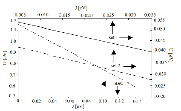
Figure 1: Lines in $U,J$ parameter space which reproduce the resonance energy of 0.04 eV. The H$\&$C line has been calculated using the set of parameters given in Ref. [HC, ], while set 1 and set 2 are obtained by using the two sets of parameters given in Ref. [N, ].

In Fig. 1 we present the results of our calculations of the lines in $U,J$ parameter space which reproduce the resonance energy of 40 meV using all twenty channels but with set 1, set 2 and H$\&$C parameters. Perhaps due to the limited size of single crystals currently available, no incommensurate peaks in Bi2212 samples have been reported so far. To obtain the exact values of the strengths we need at least one IC peak.

Strengths of interactions in $YBa_{2}Cu_{3}O_{6.7}$ samples. To obtain the strengths of the interactions we use the commensurate peak at $\sim 40$ meV and incommensurate peaks at $\sim 24$ meV and $\sim 32$ meV which have been reported in underdoped $YBa_{2}Cu_{3}O_{6.7}$ Ar . It is known that the YBaCuO is a two-layer material, but most of the peak structures associated with the neutron cross section can be captured by one layer band calculations DD . The effects due to the two-layer structure can, in principle, be incorporated in our approach, but this will make the corresponding numerical calculations much more complicated.

The commensurate and incommensurate peak structures associated with the neutron cross section in YBaCuO have been studied within the electron-hole scenario using the single-band Hubbard $t-U$ model Mc ; Sch ; Er or the $t-J$ model MW ; BL ; BL1 ; Li ; Li1 ; YM . The techniques that have been used are based on (i) the Monte Carlo numerical calculations Mc , (ii) the random phase approximation (RPA) for the magnetic susceptibility Sch ; Er , (iii) the mean-field approximation MW ; BL and (iv) the RPA combined with the slave-boson mean field scheme BL1 ; Li ; Li1 ; YM . It is known that in the case when the Hubbard repulsion is large ($U/t\rightarrow\infty$), the antiferromagnetic exchange $J$ interaction is the consequence of Hubbard repulsion, because the $t-J$ model is obtained after projecting out the doubly occupied states in the Hubbard $t-U$ model, so that $J=2t^{2}/U$. Strictly speaking, by projecting out the doubly occupied states we remove the high-energy degrees of freedom and replace them with kinematical constraints assuming that the high energy scale (given by $U$ that in cuprates corresponds to the energy cost to doubly occupy the same site) is irrelevant. Thus, if the constraint of no double occupancy is released, we arrive to the conclusion that the the magnetic susceptibility should be calculated using the $t-U-J$ model rather than the $t-U$ and $t-J$ models (the corresponding arguments are presented in Refs. [K, ; J, ; K1, ; X, ]).

In our calculations the mean-field electron energy $\overline{\varepsilon}_{\textbf{k}}$ has a tight-binding form $\overline{\varepsilon}_{\textbf{k}}=-2t\left(\cos k_{x}+\cos k_{y}\right)+4t^{\prime}\cos k_{x}\cos k_{y}-2t^{\prime\prime}(\cos 2k_{x}+\cos 2k_{y})-\mu$ . Using the established approximate parabolic relationship $T_{c}/T_{c,max}=1-82.6(p-0.16)^{2}$, where $Tc,max\sim 93$K is the maximum transition temperature of the system, $T_{c}=67$K is the transition temperature for underdoped $YBa_{2}Cu_{3}O_{6.7}$, we find that the hole doping is $p=0.10$. At that level of doping the ARPES parameters are obtained in Refs. [ARPES, ]: $t=0.25$ eV, $t^{\prime}=0.4t$, $t^{\prime\prime}=0.0444t$ and $\mu=-0.27$ eV. In the case of d-pairing the gap function is $\Delta_{\textbf{k}}=\Delta d_{\textbf{k}}/2$, where the gap maximum $\Delta$ should agree with ARPES experiments. In the case of underdoped $YBa_{2}Cu_{3}O_{6.7}$ the gap maximum has to be between the corresponding $\Delta=66$ meV in $YBa_{2}Cu_{3}O_{6.6}$ and $\Delta=50$ meV in $YBa_{2}Cu_{3}O_{6.95}$ Delta , so we set $\Delta=60$ meV. The numerical solution of the gap equation provides $V_{\psi}=265$ meV. Next, we have solved numerically the BS equations to obtain the spectrum of the collective modes $\omega(\textbf{Q})$ at the commensurate point $\textbf{Q}_{AF}$, as well as at four incommensurate points $\pi(1\pm\delta),\pi)$ and $\pi,\pi(1\pm\delta))$. From the 40 meV solution of the BS equations at $\textbf{Q}_{AF}$ we obtain a relation between $U$ and $J$ parameters, which is represented by the linear formula $U=-3.985J+1.01$ ($U$ and $J$ are in eV). By means of the last relation we have solved the BS equations for the one of the four incommensurate 24 meV peaks ($\delta=0.22$). Ar The solution provides the following interaction strengths: $J\sim 129$ meV, $V\sim 35.7$ meV and $U\sim 495$ meV. To test the above values of the strengths we calculated the positions of the incommensurate peaks at 32 meV ($\delta=0.19$).Ar The BS equations with the above strengths provide the deviation from $\textbf{Q}_{AF}$ of about $\delta=0.192$, which is in excellent agreement with the experimentally obtained deviation (see FIG. 2 in Ref. [Ar, ]). The strength of $J$ is in a very good agreement with the strength of the superexchange interactions in the underdoped antiferromagnetic insulator state of the cuprates which in YBaCO family has a magnitude of $0.1-0.12$ eV, though some theoretical papers have predicted similar magnitudes.

Strengths of interactions in $La_{2-0.16}Sr_{0.16}CuO_{4}$ samples. To obtain the strengths of the interactions we use two IC peaks at $\sim 7.1$ meV ($\delta=0.261$) and at $\sim 10$ meV ($\delta=0.255$) which have been reported in Refs. [CH, ]. The tight-binding band parameters interpolated from values given in Refs. [Tbp, ]: $t=0.25$ eV, $t^{\prime}=0.148t$, $t^{\prime\prime}=-0.5t$ and $\mu=-0.821t$. The maximum energy gap (estimated according to the prediction of the mean-field theoryMFG ) is about 10 meV, and therefore, $V_{\psi}=95.8$ meV, which corresponds to maximum value of $J$ about 64 meV. The solutions of the BS equations provide the following interaction strengths: $J\sim 44.1$ meV, $V\sim 14.8$ meV and $U\sim 442.5$ meV. To test these parameters we calculated the position of the IC peak at 18 meV. The calculated value of $\delta=0.19$ is in very good agreement with the experimental value of $\delta=0.186$.CH The above strengths provide the position of the commensurate peak to be at $\sim 40$ meV, which is in a very good agreement with the experimental value of $41\pm 2.5$ meV.CH It is worth mentioning that in $La_{2}CuO_{4}$ $J\sim 120$ meV, and therefore, our calculations support the idea that the antiferromagnetic interaction decreases with doping.DJ
Conclusion Our approach to the incommensurate and commensurate structure of the magnetic susceptibility is based on the conventional idea of particle-hole excitations around the Fermi surface. There exists a second interpretation of the structure of the magnetic susceptibility in terms of the spin-charge stripe scenario (see Ref. [Str, ] and the references therein) according to which the incommensurate peaks are natural descendants of the stripes, which are complex patterns formed by electrons confined to separate linear regions in the crystal. We do not wish to repeat the theoretical arguments that were advanced against the stripes model, but our unified description of the peaks based on the $t-U-V-J$ model strongly supports the idea put forward by various groups that the commensurate resonance and the incommensurate peaks in cuprate compounds have a common origin.

References

• (1) J. Rossat-Mignond, L. P. Regnault, C. Vettier, P. Bourges, P. Burlet, J. Bossy, J. Y. Henry, and G. Lapertot, Physica C 185- 189, 86 (1991); H. A. Mook , M. Yethiraj, G. Aeppli, T. E. Mason, and T. Armstrong, Phys. Rev. Lett. 70, 3490 (1993); P. Dai, H. A. Mook, R. D. Hunt, and F. Dogan, Phys. Rev. B 63, 054525 (2001); H. F. Fong, B. Keimer, D. Reznik, D. L. Milius, and I. A. Aksay, Phys. Rev. B 54, 6708 (1996); H. F. Fong, P. Bourges, Y. Sidis, L. P. Regnault, A. Ivanov, G. D. Gu, N. Koshizuka, and B. Keimer, Nature (London) 398, 588 (1999); H. F. Fong, P. Bourges, Y. Sidis, L. P. Regnault, J. Bossy, A. Ivanov, D. L. Milius, I. A. Aksay, and B. Keimer, Phys. Rev. B 61, 14773 (2000); P. Bourges, Y. Sidis, H. F. Fong, L. P. Regnault, J. Bossy, A. Ivanov, and B. Keimer, Science 288, 1234 (2000); H. He, P. Bourges, Y. Sidis, C. Ulrich, L. P. Regnault, S. Pailhes, N. S. Berzigiarova, N. N. Kolesnikov, and B. Keimer, Science 295, 1045 (2002).
• (2) B. FauquΓ©, Y. Sidis, L. Capogna, A. Ivanov, K. Hradil, C. Ulrich, A. I. Rykov, B. Keimer, and P. Bourges, Phys. Rev. B 76, 214512 (2007).
• (3) M. Arai, T. Nishijima, Y. Endoh, T. Egami, S. Tajima, K. Tomimoto, Y. Shiohara, M. Takahashi, A. Garrett, and S. M. Bennington, Phys. Rev. Lett. 83, 608 (1999).
• (4) W. C. Lee and A. H. MacDonald, Phys. Rev. B, 78, 174506 (2008).
• (5) W. C. Lee, J. Sinova, A. A. Burkov, Y. Joglekar, and A. H. MacDonald, Phys. Rev. B 77, 214518 (2008).
• (6) Z. Hao and A. V. Chubukov, Phys. Rev. B 79, 224513 (2009).
• (7) Z. G. Koinov and P. Nash, Phys. Rev. B 82, 014528 (2010).
• (8) Z. Koinov, Phys. Stat. Sol. B 247, 140 (2010); Physica C, 470, 144 (2010).
• (9) R. CΓ΄tΓ©, and A. Griffin, Phys. Rev. B 48, 10404 (1993); Wen-Cin Wu, and A. Griffin, Phys. Rev. B 51, 1190 (1995); Phys. Rev. B 52, 7742 (1995); Z. Koinov, Phys. Rev. B 72, 085203 (2005).
• (10) N. Bulut and D. J. Scalapino, Phys. Rev. B 53, 5149 (1996).
• (11) M. R. Norman, Phys. Rev. B, 61, 14751 (2000).
• (12) Q. M. Si, Y. Y. Zha, K. Levin, and J. P. Lu, Phys. Rev. B 47, 9055 (1993); D. Z. Liu, Y. Zha, and K. Levin, Phys. Rev. Lett. 75, 4130 (1995).
• (13) C. Buhler and A. Moreo, Phys. Rev. B 59, 9882 (1999).
• (14) A. P. Schnyder, A. Bill, C. Mudry, R. Gilardi, H. M. R nnow, and J. Mesot, Phys. Rev. B 70, 214511 (2004).
• (15) I. Eremin, D. K. Morr, A.V. Chubukov, K. H. Bennemann, and M. R. Norman, Phys. Rev. Lett. 94, 147001 (2005).
• (16) K. Maki, and H. Won, Phys. Rev. Leet., 72,1758 (1994).
• (17) J. Brinckmann and P. A. Lee, Phys. Rev. B 65, 014502 (2001).
• (18) J. Brinckmann, and P. A. Lee, Phys. Rev. Lett., 82, 2915 (1999).
• (19) Jian-Xin Li, Chung-Yu Mou, and T. K. Lee, Phys. Rev. B 62, 640 (2000).
• (20) Jian-Xin Li, and Chang-De Gong, Phys. Rev. B 66, 014506 (2002).
• (21) H. Yamase and W. Metzner, Phys. Rev. B 73, 214517 (2006).
• (22) T. K. KopeΔ‡, Phys. Rev. B 70, 054518 (2004).
• (23) J. Dai J, X. Feng, T. Xiang and Y. Yu Phys. Rev. B 70, 064518 (2004).
• (24) T. K. KopeΔ‡, Phys. Rev. B 73, 104505 (2006).
• (25) T. Xiang T, H. G. Luo, D. H. Lu, K. M. Shen and Z. X. Shen, Phys. Rev. B 79, 014524 (2009).
• (26) I. Dimov, P. Goswami, X. Jia, and S. Chakravarty, Phys. Rev. B 78, 134529 (2008); P. Goswami, Phys. Stat. Sol. (B) 247, 595 (2010).
• (27) M. Sutherland, D. G. Hawthorn, R. W. Hill, F. Ronning, S. Wakimoto, H. Zhang, C. Proust, E. Boaknin, C. Lupien, L. Taillefer, R. Liang, D. A. Bonn, W. N. Hardy, R. Gagnon, N. E. Hussey, T. Kimura, M. Nohara, and H. Takagi, Phys. Rev. B 67, 174520 (2003).
• (28) N. B. Christensen, D. F. McMorrow, H.M. R nnow, B. Lake, S.M. Hayden, G. Aeppli, T.G. Perring, M. Mangkorntong, M. Nohara, and H. Takagi, Phys. Rev. Lett., 93,147002 (2007); B. Vignolle, S. M. Hayden, D. F. McMorrow, H. M. RΓΈnnow, B. Lake, C. D. Frost and T. G. Perring, Nature physics 3, 163 (2007).
• (29) T. Yoshida, X. J. Zhou, K. Tanaka, W. L. Yang, Z. Hussain, Z.-X. Shen, A. Fujimori, S. Sahrakorpi, M. Lindroos, R. S. Markiewicz, A. Bansil, Seiki Komiya, Yoichi Ando, H. Eisaki, T. Kakeshita, and S. Uchida Phys. Rev. B 74, 224510 (2006); T. Yoshida, X.J. Zhou, D.H. Lu, S. Komiya, Y. Ando, H. Eisaki, T. Kakeshita, S. Uchida, Z. Hussain, Z-X Shen and A. Fujimori J. Phys.: Condens. Matter 19, 125209 (2007); A. Narduzzo, G. Albert, M. M. J. French, N. Mangkorntong, M. Nohara, H. Takagi, and N. E. Hussey, Phys. Rev. B 77, 220502(R) (2008).
• (30) H. Won and K. Maki, Phys. Rev. B 49, 1397 (1994); A. Ino, C. Kim, M. Nakamura, T. Yoshida, T. Mizokawa, A. Fujimori, Z.-X. Shen, T. Kakeshita, H. Eisaki, and S. Uchida Phys. Rev. B 65, 094504 (2002).
• (31) D. C. Johnson, Phys. Rev. Leet., 62, 957 (1989).
• (32) S. A. Kivelson, I. P. Bindloss, E. Fradkin, V. Oganesyan, J. M. Tranquada, A. Kapitulnik, and C. Howald, Rev. Mod. Phys. 75, 1201 (2003).