Bethe-Salpeter equations for the collective modes of the $t-U-V-J$ model with d-wave pairing

Abstract

The Bethe-Salpeter equations for the collective modes of a $t$-$U$-$V$-$J$ model are used to analyze the resonance peak observed at $\bf{Q}=(\pi,\pi)$ in neutron scattering experiments on the cuprates. We assume that the resonance emerges due to the mixing between the spin channel and 19 other channels. We have calculated the energy of the lowest mode of the extended Hubbard model ($J=0$) vs the on-site repulsive interaction $U$, as well as the $UJ$ lines in the interaction parameter space which are consistent with the ARPES data and reproduces the resonance peak at 40 meV in Bi2212 compound. We find that the resonance is predominantly a spin exciton.

Introduction. It is widely accepted that: (i) the angle-resolved photoemission spectroscopy (ARPES) data produce evidences for the opening of a d-wave pairing gap in cuprates compounds described at low energies and temperatures by a BCS theory, and (ii) the basic pairing mechanism arises from the antiferromagnetic exchange correlations, but the charge fluctuations associated with double occupancy of a site also play an essential role in doped systems. The simplest model that is consistent with the last statements is the $t$-$U$-$V$-$J$ model. In the case of d-pairing the gap function is $\Delta_{\textbf{k}}=\Delta d_{\textbf{k}}/2$, where $\Delta$ is the maximum value of the energy gap and $d_{\textbf{k}}=(\cos k_{x}-\cos k_{y})$ (lattice constant $a=1$). The BCS gap equation is $1=\frac{V_{\psi}}{2}\int^{\pi}_{-\pi}\int^{\pi}_{-\pi}\frac{d\textbf{k}}{(2\pi)^{2}}\frac{d^{2}_{\textbf{k}}}{\sqrt{\overline{\varepsilon}^{2}_{\textbf{k}}+\Delta^{2}_{\textbf{k}}}}$, where $V_{\psi}=2V+3J/2$, $E(\textbf{k})=\sqrt{\overline{\varepsilon}^{2}_{\textbf{k}}+\Delta^{2}_{\textbf{k}}}$. The mean-field electron energy $\overline{\varepsilon}_{\textbf{k}}$ has a tight-binding form $\overline{\varepsilon}_{\textbf{k}}=t_{1}\left(\cos k_{x}+\cos k_{y}\right)/2+t_{2}\cos k_{x}\cos k_{y}+t_{3}(\cos 2k_{x}+\cos 2k_{y})/2+t_{4}(\cos 2k_{x}\cos k_{y}+\cos 2k_{y}\cos k_{x})/2+t_{5}\cos 2k_{x}\cos 2k_{y}-\mu$ obtained by fitting the ARPES data with a chemical potential $\mu$ and hopping amplitudes $t_{i}$ for first to fifth nearest neighbors on a square lattice. $\Delta$, $t_{1},...,t_{5}$ and $\mu$ should all be thought of as an effective set of parameters, while $V_{\psi}$ has to be determined by the gap equation. For Bi2212 compound, there are two possible sets of parameters with all tight-binding basis functions involved (see Table 1 in Ref. [N, ]). Assuming $\Delta=35$ meV, we obtain $V^{(1)}_{\psi}=115.2$ meV with set 1, and $V^{(2)}_{\psi}=87.9$ meV with set 2. Hao and ChubukovHC have used another set of parameters (we shall call it H$\&$C) for Bi2212 compound with a doping concentration $x=0.12$: $t_{1}=-4t,t_{2}=1.2t$, $t=0.433$ eV, $\mu=-0.94t$, $\Delta=35$ meV and $V_{\psi}=0.6t$. The parameters $U,V$ and $J$ should be adjusted in such a way that the sharp collective mode which appears at wave vector $\textbf{Q}_{0}=(\pi,\pi)$ in inelastic neutron-scattering resonance (INSR) studiesNSS occurs at energy which corresponds to the lowest collective mode of the corresponding Hamiltonian. In RPA the resonance is determined by the pole of the spin correlation function, which in the case of $J=0$ (the phase diagram at half filling shows an ”island” in U-V space where d-wave pairing existsD ) is: $\chi_{s}(\omega)=\chi^{0}_{00}(\textbf{Q}_{0},\omega)/[1+U\chi^{0}_{00}(\textbf{Q}_{0},\omega)]$, where the bare spin correlation functionBS ; N is $\chi^{0}_{00}=I_{\widetilde{\gamma}\widetilde{\gamma}}$ ($I_{\widetilde{\gamma}\widetilde{\gamma}}$ is defined later in the text). Using the H$\&$C set of parametersHC and a resonance energy of 40 meV, we calculate the RPA value of $U$ of about 1.16 eV. Sets 1 and 2 provide $U^{(1)}=0.533$ eV and $U^{(2)}=0.418$ eV, respectively. The coupling of the spin channel with other channels should change the RPA results for $U$. For example, we have two $\pi$ channelsExc with bare $\pi$ susceptibilities $\chi^{0}_{11}=I^{22}_{ll}$ and $\chi^{0}_{22}=I^{22}_{\gamma\gamma}$, respectively. The susceptibilities $I^{2}_{\gamma\widetilde{\gamma}},J^{2}_{l\widetilde{\gamma}},J^{22}_{l\gamma}$ represent the mixing of the spin and two $\pi$ channels. Thus, the coupling of the spin and two $\pi$ channels (a three-channel response-function theory) leads in the generalized random phase approximation (GRPA) to a set of three coupled equations,HC and the value of $U$ is reduced from 1.16 eV to 0.974 eV. When the extended spin channel is added to the previous three channels, we have a set of four coupled equations (a four-channel theory), and according to Ref. [Plas, ] $U\approx 300$ meV is required in the case when $V_{\psi}$=0.260 eV and $J=0$.

In what follows, the energy of the resonance is obtained from the solution of 20 coupled Bethe-Salpeter (BS) equations for the collective modes in GRPA, i.e. the resonance emerges due to the mixing between the spin channel and other 19 channels. In our approach the INSR energy solves $det|\widehat{\chi}^{-1}-\widehat{V}|=0$, where the mean-field response function $\widehat{\chi}$ and the interaction $\widehat{V}$ are $20\times 20$ matrices. The secular determinant can be rewritten as $det|\widehat{\chi}^{-1}-\widehat{V}|=det\left|\begin{array}[]{cc}A&B\\ B^{T}&C\end{array}\right|=det|C|det|A-BC^{-1}B^{T}|$. In the case of the four-channel response-function theory,Plas ; Plas1 $A$ is a $4\times 4$ matrix while the mixing with the other 16 channels is represented by a $4\times 4$ matrix $BC^{-1}B^{T}$. We emphasize that none of the previous theoretical interpretations of the INSR feature at $\textbf{Q}_{0}$ have accounted properly for the mixing term $BC^{-1}B^{T}$.

t-U-V-J model. The Hamiltonian of the $t$-$U$-$V$-$J$ model consists of $t$ and $U$ terms representing the hopping of electrons between sites of the lattice and their on-site repulsive interaction, as well as the spin-independent attractive interaction $V$ and the spin-dependent antiferromagnetic interaction $J$:

$$\begin{split}&H=-\sum_{i,j,\sigma}t_{ij}\psi^{\dagger}_{i,\sigma}\psi_{j,\sigma}-\mu\sum_{i,\sigma}\widehat{n}_{i,\sigma}+U\sum_{i}\widehat{n}_{i,\uparrow}\widehat{n}_{i,\downarrow}\\ &-V\sum_{<i,j>\sigma\sigma^{\prime}}\widehat{n}_{i,\sigma}\widehat{n}_{j,\sigma^{\prime}}+J\sum_{<i,j>}\overrightarrow{\textbf{S}}_{i}\textbf{.}\overrightarrow{\textbf{S}}_{j}.\end{split}$$ (1)

Here, the Fermi operator $\psi^{\dagger}_{i,\sigma}$ ($\psi_{i,\sigma}$) creates (destroys) a fermion on the lattice site $i$ with spin projection $\sigma=\uparrow,\downarrow$ along a specified direction and $\widehat{n}_{i,\sigma}=\psi^{\dagger}_{i,\sigma}\psi_{i,\sigma}$ is the density operator on site $i$ with a position vector $\textbf{r}_{i}$. The symbol $\sum_{<ij>}$ means sum over nearest-neighbor sites. $t_{ij}$ is the single electron hopping integral. The antiferromagnetic spin-dependent interaction $J\sum_{<i,j>}\overrightarrow{\textbf{S}}_{i}\textbf{.}\overrightarrow{\textbf{S}}_{j}=J_{1}+J_{2}$ consists of two terms: $J_{1}=\frac{J}{4}\sum_{<i,j>}[\widehat{n}_{i,\uparrow}\widehat{n}_{j,\uparrow}+\widehat{n}_{i,\downarrow}\widehat{n}_{j,\downarrow}-\widehat{n}_{i,\uparrow}\widehat{n}_{j,\downarrow}-\widehat{n}_{i,\downarrow}\widehat{n}_{j,\uparrow}]$ and $J_{2}=\frac{J}{2}\sum_{<i,j>}\left[\psi^{\dagger}_{i,\uparrow}\psi_{i,\downarrow}\psi^{\dagger}_{j,\downarrow}\psi_{j,\uparrow}+\psi^{\dagger}_{i,\downarrow}\psi_{i,\uparrow}\psi^{\dagger}_{j,\uparrow}\psi_{j,\downarrow}\right]$.

It is useful to introduce four-component Nambu fermion fields $\widehat{\overline{\psi}}(y)=\left(\psi^{\dagger}_{\uparrow}(y)\psi^{\dagger}_{\downarrow}(y)\psi_{\uparrow}(y)\psi_{\downarrow}(y)\right)$ and $\widehat{\psi}(x)=\left(\psi^{\dagger}_{\uparrow}(x)\psi^{\dagger}_{\downarrow}(x)\psi_{\uparrow}(x)\psi_{\downarrow}(x)\right)^{T}$, where $x$ and $y$ are composite variables and the field operators obey anticommutation relations. The ”hat” symbol over any quantity $\widehat{O}$ means that this quantity is a matrix.

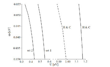
Figure 1: The energy of the resonance obtained from the BS equations when $J=0$. The curves are plotted using parameters given in Table 1 in Ref. [N, ] (set 1 and set 2), and the Hao and Chubukov parameters (curves H$\&$C). The puncture curve represents the three-channel energy (Fig. 4 in Ref. [HC, ]).

The interaction part of the extended Hubbard Hamiltonian is quartic in the Grassmann fermion fields so the functional integrals cannot be evaluated exactly. However, we can transform the quartic terms to a quadratic form by applying the Hubbard-Stratonovich transformation for the electron operators:ZK1 $\int DAe^{\left[\frac{1}{2}A_{\alpha}(z)D_{\alpha\beta}^{(0)-1}(z,z^{\prime})A_{\beta}(z)+\widehat{\overline{\psi}}(y)\widehat{\Gamma}^{(0)}_{\alpha}(y;x|z)\widehat{\psi}(x)A_{\alpha}(z)\right]}=e^{-\frac{1}{2}\widehat{\overline{\psi}}(y)\widehat{\Gamma}^{(0)}_{\alpha}(y;x|z)\widehat{\psi}(x)D_{\alpha\beta}^{(0)}(z,z^{\prime})\widehat{\overline{\psi}}(y^{\prime})\widehat{\Gamma}^{(0)}_{\beta}(y^{\prime};x^{\prime}|z^{\prime})\widehat{\psi}(x^{\prime})}$. The last equation is used to define the $4\times 4$ matrices $\widehat{D}_{\alpha\beta}^{(0)}$ and $\widehat{\Gamma}^{(0)}_{\alpha}$ ($\alpha,\beta=1,2,3,4$). Their Fourier transforms, written in terms of the Pauli $\sigma_{i}$, Dirac $\gamma^{0}$ and alphaY ; B matrices, are as follows: $\widehat{D}^{(0)}=\left(\begin{array}[]{cc}\widehat{D}_{1}&0\\ 0&\widehat{D}_{2}\end{array}\right)$, $\widehat{\Gamma}_{1,2}^{(0)}=(\gamma^{0}\pm\alpha_{z})/2$ and $\widehat{\Gamma}_{3,4}^{(0)}=(\alpha_{x}\pm\imath\alpha_{y})/2$, where $\alpha_{i}=\left(\begin{array}[]{cc}\sigma_{i}&0\\ 0&\sigma_{y}\sigma_{i}\sigma_{y}\end{array}\right)$, $\widehat{D}_{1}=\left(J(\textbf{k})-V(\textbf{k})\right)\sigma_{0}+\left(U-J(\textbf{k})-V(\textbf{k})\right)\sigma_{x}$ and $\widehat{D}_{2}=2J(\textbf{k})\sigma_{x}$. For a square lattice and nearest-neighbor interactions $V(\textbf{k})=4V(\cos(k_{x})+\cos(k_{y}))$ and $J(\textbf{k})=J(\cos(k_{x})+\cos(k_{y}))$. Now, we can establish a one-to-one correspondence between the system under consideration and a system which consists of a four-component boson field $A_{\alpha}(z)$ interacting with fermion fields $\widehat{\overline{\psi}}(y)$ and $\widehat{\psi}(x)$. The action of the model system is $S=S^{(e)}_{0}+S^{(A)}_{0}+S^{(e-A)}$ where: $S^{(e)}_{0}=\widehat{\overline{\psi}}(y)\widehat{G}^{(0)-1}(y;x)\widehat{\psi}(x)$, $S^{(A)}_{0}=\frac{1}{2}A_{\alpha}(z)D^{(0)-1}_{\alpha\beta}(z,z^{\prime})A_{\beta}(z^{\prime})$ and $S^{(e-A)}=\widehat{\overline{\psi}}(y)\widehat{\Gamma}^{(0)}_{\alpha}(y,x\mid z)\widehat{\psi}(x)A_{\alpha}(z)$. Here, we have used composite variables $x,y,z=\{\textbf{r}_{i},u\}$, where $\textbf{r}_{i}$ is a lattice site vector, and variable $u$ range from $0$ to $\beta=1/k_{B}T$ ($T$ and $k_{B}$ are the temperature and the Boltzmann constant). We set $\hbar=1$ and we use the summation-integration convention: that repeated variables are summed up or integrated over.

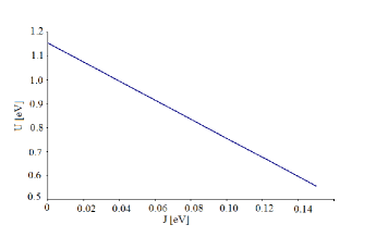
Figure 2: Line in $U,J$ parameter space which reproduce the INSR energy of 0.04 eV. Note that $V=V_{\psi}/2-3J/4$ where $V_{\psi}=0.6t=259.8$ meV is calculated from the gap equation by using the set of parameters given in Ref. [HC, ].

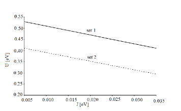
Figure 3: Line in $U,J$ parameter space which reproduce the INSR energy of 0.04 eV. The $V$ value is $V=V_{\psi}/2-3J/4$ where $V^{(1)}_{\psi}=115.2$ meV and $V^{(2)}_{\psi}=87.9$ meV are calculated by using two sets of parameters given in Ref. [N, ].

Following the same steps as in Refs. [GFS, ; ZK, ], we can derive a set of sixteen BS equations for the collective mode $\omega(\textbf{Q})$ and BS amplitudes $\Psi^{\textbf{Q}}_{n_{1}n_{2}}(\textbf{k})$ ($n_{1},n_{2}=1,2,3,4$). Their matrix representation at zero temperature is :

$$\begin{split}&\widehat{\Psi}^{\textbf{Q}}(\textbf{k})=\frac{1}{N}\sum_{\textbf{q}}\int\frac{d\Omega}{2\pi}\{-\widehat{D}^{(0)}_{\alpha\beta}(\textbf{k}-\textbf{q})\widehat{G}(\textbf{k}+\textbf{Q};\Omega+\omega)\\ &\widehat{\Gamma}^{(0)}_{\alpha}\widehat{\Psi}^{\textbf{Q}}(\textbf{q})\widehat{\Gamma}^{(0)}_{\beta}\widehat{G}(\textbf{k};\Omega)+\widehat{D}^{(0)}_{\alpha\beta}(\textbf{Q})\widehat{G}(\textbf{k}+\textbf{Q};\Omega+\omega)\\ &\widehat{\Gamma}^{(0)}_{\alpha}\widehat{G}(\textbf{k};\Omega)Tr[\widehat{\Gamma}^{(0)}_{\beta}\widehat{\Psi}^{\textbf{Q}}(\textbf{q})]\},\end{split}$$ (2)

where $\widehat{G}(\textbf{k};\omega)$ is the BCS Green’s function.Y ; B The direct $\widehat{D}^{(0)}_{\alpha\beta}(\textbf{k}-\textbf{q})\widehat{\Gamma}^{(0)}_{\alpha}\widehat{\Gamma}^{(0)}_{\beta}$ and exchange $\widehat{D}^{(0)}_{\alpha\beta}(\textbf{Q})\widehat{\Gamma}^{(0)}_{\alpha}\widehat{\Gamma}^{(0)}_{\beta}$ interactions mix all sixteen BS amplitudes. We can greatly simplify Eqs. (2) using the fact that in the RPA the susceptibilities at $\textbf{Q}_{0}$ are convolutions of two single-particle Green’s functions $\widehat{G}$, and the equation for the collective mode in the RPA is: $\chi^{(0)-1}_{1}(\omega)\chi^{(0)-1}_{2}(\omega)-C_{12}(\omega)=0$, where the susceptibilities $\chi^{(0)}_{1}$ and $\chi^{(0)}_{2}$ originate from ($U,J_{1}$) and $J_{2}$ interactions, respectively. The term $C_{12}$ mixes the $J_{1}$ and $J_{2}$ interactions, but it is proportional to convolutions which involve the anomalous Green’s functions $G_{13}$ and $G_{24}$. The two Green’s functions appears in the case of spin triplet pairing states where the order parameter $\Delta_{\alpha\beta}(\textbf{k})$ is a $2\times 2$ matrix. For a singlet superconductivity and d-wave pairing $\Delta_{\alpha\beta}(\textbf{k})=i(\sigma_{y})_{\alpha\beta}\Delta(\textbf{k})$, $C_{12}(\omega)=0$, and the equation for collective modes becomes $\left[1+(U+4J)I_{\widetilde{\gamma}\widetilde{\gamma}}\right]\left[1+4JI_{\widetilde{\gamma}\widetilde{\gamma}}\right]=0$, i.e. $J_{1}$ and $J_{2}$ terms contribute separately to the collective modes. Thus, we shall neglect all contributions due to the $J_{2}$ term in Eqs. (2). In this approximation we have a set of four equations, which can be further simplified to a set of two equations in the same manner as in Refs. [GFS, ; ZK, ]:

$$\begin{split}&[\omega(\textbf{Q})-\varepsilon(\textbf{k},\textbf{Q})]G^{+}(\textbf{k},\textbf{Q})=\frac{U}{2N}\sum_{\textbf{q}}\left[\gamma_{\textbf{k},\textbf{Q}}\gamma_{\textbf{q},\textbf{Q}}+l_{\textbf{k},\textbf{Q}}l_{\textbf{q},\textbf{Q}}\right]G^{+}(\textbf{q},\textbf{Q})-\frac{U}{2N}\sum_{\textbf{q}}\left[\gamma_{\textbf{k},\textbf{Q}}\gamma_{\textbf{q},\textbf{Q}}-l_{\textbf{k},\textbf{Q}}l_{\textbf{q},\textbf{Q}}\right]G^{-}(\textbf{q},\textbf{Q})\\ &-\frac{1}{2N}\sum_{\textbf{q}}\left[V(\textbf{k}-\textbf{q})+J(\textbf{k}-\textbf{q})\right]\left[\gamma_{\textbf{k},\textbf{Q}}\gamma_{\textbf{q},\textbf{Q}}+l_{\textbf{k},\textbf{Q}}l_{\textbf{q},\textbf{Q}}\right]G^{+}(\textbf{q},\textbf{Q})\\ &-\frac{1}{2N}\sum_{\textbf{q}}\left[V(\textbf{k}-\textbf{q})-J(\textbf{k}-\textbf{q})\right]\left[\widetilde{\gamma}_{\textbf{k},\textbf{Q}}\widetilde{\gamma}_{\textbf{q},\textbf{Q}}+m_{\textbf{k},\textbf{Q}}m_{\textbf{q},\textbf{Q}}\right]G^{+}(\textbf{q},\textbf{Q})\\ &+\frac{1}{2N}\sum_{\textbf{q}}\left[V(\textbf{k}-\textbf{q})+J(\textbf{k}-\textbf{q})\right]\left[\gamma_{\textbf{k},\textbf{Q}}\gamma_{\textbf{q},\textbf{Q}}-l_{\textbf{k},\textbf{Q}}l_{\textbf{q},\textbf{Q}}\right]G^{-}(\textbf{q},\textbf{Q})\\ &+\frac{1}{2N}\sum_{\textbf{q}}\left[V(\textbf{k}-\textbf{q})-J(\textbf{k}-\textbf{q})\right]\left[\widetilde{\gamma}_{\textbf{k},\textbf{Q}}\widetilde{\gamma}_{\textbf{q},\textbf{Q}}-m_{\textbf{k},\textbf{Q}}m_{\textbf{q},\textbf{Q}}\right]G^{-}(\textbf{q},\textbf{Q})\\ &-\frac{U-2J(\textbf{Q})}{2N}\sum_{\textbf{q}}\widetilde{\gamma}_{\textbf{k},\textbf{Q}}\widetilde{\gamma}_{\textbf{q},\textbf{Q}}\left(G^{+}(\textbf{q},\textbf{Q})-G^{-}(\textbf{q},\textbf{Q})\right)+\frac{U-2V(\textbf{Q})}{2N}\sum_{\textbf{q}}m_{\textbf{k},\textbf{Q}}m_{\textbf{q},\textbf{Q}}\left[G^{+}(\textbf{q},\textbf{Q})+G^{-}(\textbf{q},\textbf{Q})\right],\end{split}$$ (3)

$$\begin{split}&[\omega(\textbf{Q})+\varepsilon(\textbf{k},\textbf{Q})]G^{-}(\textbf{k},\textbf{Q})=-\frac{U}{2N}\sum_{\textbf{q}}\left[\gamma_{\textbf{k},\textbf{Q}}\gamma_{\textbf{q},\textbf{Q}}+l_{\textbf{k},\textbf{Q}}l_{\textbf{q},\textbf{Q}}\right]G^{-}(\textbf{q},\textbf{Q})+\frac{U}{2N}\sum_{\textbf{q}}\left[\gamma_{\textbf{k},\textbf{Q}}\gamma_{\textbf{q},\textbf{Q}}-l_{\textbf{k},\textbf{Q}}l_{\textbf{q},\textbf{Q}}\right]G^{+}(\textbf{q},\textbf{Q})\\ &+\frac{1}{2N}\sum_{\textbf{q}}\left[V(\textbf{k}-\textbf{q})+J(\textbf{k}-\textbf{q})\right]\left[\gamma_{\textbf{k},\textbf{Q}}\gamma_{\textbf{q},\textbf{Q}}+l_{\textbf{k},\textbf{Q}}l_{\textbf{q},\textbf{Q}}\right]G^{-}(\textbf{q},\textbf{Q})\\ &+\frac{1}{2N}\sum_{\textbf{q}}\left[V(\textbf{k}-\textbf{q})-J(\textbf{k}-\textbf{q})\right]\left[\widetilde{\gamma}_{\textbf{k},\textbf{Q}}\widetilde{\gamma}_{\textbf{q},\textbf{Q}}+m_{\textbf{k},\textbf{Q}}m_{\textbf{q},\textbf{Q}}\right]G^{-}(\textbf{q},\textbf{Q})\\ &-\frac{1}{2N}\sum_{\textbf{q}}\left[V(\textbf{k}-\textbf{q})+J(\textbf{k}-\textbf{q})\right]\left[\gamma_{\textbf{k},\textbf{Q}}\gamma_{\textbf{q},\textbf{Q}}-l_{\textbf{k},\textbf{Q}}l_{\textbf{q},\textbf{Q}}\right]G^{+}(\textbf{q},\textbf{Q})\\ &-\frac{1}{2N}\sum_{\textbf{q}}\left[V(\textbf{k}-\textbf{q})-J(\textbf{k}-\textbf{q})\right]\left[\widetilde{\gamma}_{\textbf{k},\textbf{Q}}\widetilde{\gamma}_{\textbf{q},\textbf{Q}}-m_{\textbf{k},\textbf{Q}}m_{\textbf{q},\textbf{Q}}\right]G^{+}(\textbf{q},\textbf{Q})\\ &-\frac{U-2J(\textbf{Q})}{2N}\sum_{\textbf{q}}\widetilde{\gamma}_{\textbf{k},\textbf{Q}}\widetilde{\gamma}_{\textbf{q},\textbf{Q}}\left(G^{+}(\textbf{q},\textbf{Q})-G^{-}(\textbf{q},\textbf{Q})\right)-\frac{U-2V(\textbf{Q})}{2N}\sum_{\textbf{q}}m_{\textbf{k},\textbf{Q}}m_{\textbf{q},\textbf{Q}}\left[G^{+}(\textbf{q},\textbf{Q})+G^{-}(\textbf{q},\textbf{Q})\right].\end{split}$$ (4)

Here $\varepsilon(\textbf{k},\textbf{Q})=E(\textbf{k}+\textbf{Q})+E(\textbf{k})$, and we use the same form factors as in Ref.[GFS, ]: $\gamma_{\textbf{k},\textbf{Q}}=u_{\textbf{k}}u_{\textbf{k}+\textbf{Q}}+v_{\textbf{k}}v_{\textbf{k}+\textbf{Q}},\quad l_{\textbf{k},\textbf{Q}}=u_{\textbf{k}}u_{\textbf{k}+\textbf{Q}}-v_{\textbf{k}}v_{\textbf{k}+\textbf{Q}},\quad\widetilde{\gamma}_{\textbf{k},\textbf{Q}}=u_{\textbf{k}}v_{\textbf{k}+\textbf{Q}}-u_{\textbf{k}+\textbf{Q}}v_{\textbf{k}},$ and $m_{\textbf{k},\textbf{Q}}=u_{\textbf{k}}v_{\textbf{k}+\textbf{Q}}+u_{\textbf{k}+\textbf{Q}}v_{\textbf{k}}$ where $u^{2}_{\textbf{k}}=1-v^{2}_{\textbf{k}}=\left[1+\overline{\varepsilon}(\textbf{k})/E(\textbf{k})\right]/2$.

It is worth mentioning that in the case of an extended Hubbard model ($J=0$), Eqs. (3) and (4) are the exact BS equations in the GRPA. They are in accordance with the Goldstone theorem which says that the gauge invariance is restored by the existence of the Goldstone mode whose energy approaches zero at $\textbf{Q}=0$. The last statement corresponds to the so-called trivial solution of the BS equations: $G^{+}(\textbf{k},\textbf{Q}=0)=-G^{-}(\textbf{k},\textbf{Q}=0)=\Delta_{\textbf{k}}/2E(\textbf{k})$, and the gap equationR $\Delta_{\textbf{k}}=\frac{1}{N}\sum_{\textbf{q}}[-U+V(\textbf{k}-\textbf{q})]\Delta_{\textbf{q}}/2E(\textbf{q})$ is recovered from our BS equations.

The Fourier transforms of $V$ and $J$ interactions are separable, i.e. $V(\textbf{k}-\textbf{q})=2V\widehat{\lambda}_{\textbf{k}}\widehat{\lambda}^{T}_{\textbf{q}}$ and $J(\textbf{k}-\textbf{q})=J\widehat{\lambda}_{\textbf{k}}\widehat{\lambda}^{T}_{\textbf{q}}/2$, and therefore, Eqs. (3) and (4) can be solved analytically. Here $\widehat{\lambda}_{\textbf{k}}=\left(s_{\textbf{k}},d_{\textbf{k}},ss_{\textbf{k}},sd_{\textbf{k}}\right)$ is an $1\times 4$ matrix, and we have used the following notations: $s_{\textbf{k}}=\cos(k_{x})+\cos(k_{y})$, $d_{\textbf{k}}=\cos(k_{x})-\cos(k_{y})$,$ss_{\textbf{k}}=\sin(k_{x})+\sin(k_{y})$ and $cd_{\textbf{k}}=\sin(k_{x})-\sin(k_{y})$. Thus, we obtain a set of 20 coupled linear homogeneous equations for the dispersion of the collective excitations. The existence of a non-trivial solution requires that the secular determinant $det\|\widehat{\chi}^{-1}-\widehat{V}\|$ is equal to zero, where the bare mean-field-quasiparticle response function $\widehat{\chi}=\left(\begin{array}[]{cc}P&Q\\ Q^{T}&R\end{array}\right)$ and the interaction $\widehat{V}=diag(U,U,-(U+4J),U+16V,-(2V+J/2),...,-(2V+J/2),-(2V-J/2),...,-(2V-J/2))$ are $20\times 20$ matrices. $P$ and $Q$ are $4\times 4$ and $4\times 16$ blocks, respectively, while $R$ is $16\times 16$ block (in what follows $i,j=1,2,3,4$):

$$P=\left|\begin{array}[]{cccc}I_{\gamma,\gamma}&J_{\gamma,l}&I_{\gamma,\widetilde{\gamma}}&J_{\gamma,m}\\ J_{\gamma,l}&I_{l,l}&J_{l,\widetilde{\gamma}}&I_{l,m}\\ I_{\gamma,\widetilde{\gamma}}&J_{l,\widetilde{\gamma}}&I_{\widetilde{\gamma},\widetilde{\gamma}}&J_{\widetilde{\gamma},m}\\ J_{\gamma,m}&I_{l,m}&J_{\widetilde{\gamma},m}&I_{m,m}\end{array}\right|,Q=\left|\begin{array}[]{cccc}I^{i}_{\gamma,\gamma}&J^{i}_{\gamma,l}&I^{i}_{\gamma,\widetilde{\gamma}}&J^{i}_{\gamma,m}\\ J^{i}_{\gamma,l}&I^{i}_{l,l}&J^{i}_{l,\widetilde{\gamma}}&I^{i}_{l,m}\\ I^{i}_{\gamma,\widetilde{\gamma}}&J^{i}_{l,\widetilde{\gamma}}&I^{i}_{\widetilde{\gamma},\widetilde{\gamma}}&J^{i}_{\widetilde{\gamma},m}\\ J^{i}_{\gamma,m}&I^{i}_{l,m}&J^{i}_{\widetilde{\gamma},m}&I^{i}_{m,m}\end{array}\right|,R=\left|\begin{array}[]{cccc}I^{ij}_{\gamma,\gamma}&J^{ij}_{\gamma,l}&I^{ij}_{\gamma,\widetilde{\gamma}}&J^{ij}_{\gamma,m}\\ J^{ij}_{\gamma,l}&I^{ij}_{l,l}&J^{ij}_{l,\widetilde{\gamma}}&I^{ij}_{l,m}\\ I^{ij}_{\gamma\widetilde{\gamma}}&J^{ij}_{l,\widetilde{\gamma}}&I^{ij}_{\widetilde{\gamma},\widetilde{\gamma}}&J^{ij}_{\widetilde{\gamma},m}\\ J^{ij}_{\gamma,m}&I^{ij}_{l,m}&J^{ij}_{\widetilde{\gamma},m}&I^{ij}_{m,m}\end{array}\right|.$$

The quantities $I_{a,b}=F_{a,b}(\varepsilon(\mathbf{k},\mathbf{Q}))$ and $J_{a,b}=F_{a,b}(\omega)$, the $1\times 4$ matrices $I^{i}_{a,b}=F^{i}_{a,b}(\varepsilon(\mathbf{k},\mathbf{Q}))$ and $J^{i}_{a,b}=F^{i}_{a,b}(\omega)$, and the $4\times 4$ matrices $I^{ij}_{a,b}=F^{ij}_{a,b}(\varepsilon(\mathbf{k},\mathbf{Q}))$ and $J^{ij}_{a,b}=F^{ij}_{a,b}(\omega)$ are defined as follows (the quantities $a(\mathbf{k},\mathbf{Q})$ and $b(\mathbf{k},\mathbf{Q})=l_{\mathbf{k},\mathbf{Q}},m_{\mathbf{k},\mathbf{Q}},\gamma_{\mathbf{k},\mathbf{Q}}$ or $\widetilde{\gamma}_{\mathbf{k},\mathbf{Q}}$):

$$F_{a,b}(x)\equiv\frac{1}{N}\sum_{\textbf{k}}\frac{xa(\mathbf{k},\mathbf{Q})b(\mathbf{k},\mathbf{Q})}{\omega^{2}-\varepsilon^{2}(\mathbf{k},\mathbf{Q})},F^{i}_{a,b}(x)\equiv\frac{1}{N}\sum_{\textbf{k}}\frac{xa(\mathbf{k},\mathbf{Q})b(\mathbf{k},\mathbf{Q})\widehat{\lambda}^{i}_{\textbf{k}}}{\omega^{2}-\varepsilon^{2}(\mathbf{k},\mathbf{Q})},F^{ij}_{a,b}(x)\equiv\frac{1}{N}\sum_{\textbf{k}}\frac{xa(\mathbf{k},\mathbf{Q})b(\mathbf{k},\mathbf{Q})}{\omega^{2}-\varepsilon^{2}(\mathbf{k},\mathbf{Q})}\left(\widehat{\lambda}^{T}_{\textbf{k}}\widehat{\lambda}_{\textbf{k}}\right)_{ij}.$$

The elements of $P,Q$ and $R$ blocks are convolutions of conventional two normal $GG$, two anomalous $FF$ Green’s functions or $FG$ terms. At the high-symmetry wave vector $\textbf{Q}_{0}$, $I_{a,b}^{i}$ and $J_{a,b}^{i}$ with $i=3,4$ involve sine functions, and therefore, all vanish. $I_{a,b}^{2}$ and $J_{a,b}^{2}$ also vanish because $\varepsilon(\mathbf{k},\mathbf{Q}_{0})$ is symmetric with respect to exchange $k_{x}\leftrightarrow k_{y}$. Similarly, the non-diagonal elements of $I_{a,b}^{ij}$ and $J_{a,b}^{ij}$ with $i\neq j$ all vanish. Thus, blocks $P$ and $Q$, each has 10 different non-zero elements, while $R$ has 40 non-zero elements. In other words, the $\omega$ dependence of $\widehat{\chi}$ (or $\widehat{\chi}^{-1}$) comes from these 60 non-zero elements. It is worth mentioning that within the four-channel theoryPlas the collective mode energy has been calculated by using a $4\times 4$ symmetric matrix $\widehat{\chi}$ which has only 6 non-zero elements at $\bf{Q}_{0}$: $\widehat{\chi}_{11}=I_{\widetilde{\gamma}\widetilde{\gamma}},\widehat{\chi}_{22}=I_{mm}^{11},\widehat{\chi}_{33}=I_{\gamma\gamma}^{22},\widehat{\chi}_{44}=I_{ll}^{22},\widehat{\chi}_{12}=J^{1}_{m\widetilde{\gamma}}$ and $\widehat{\chi}_{34}=J^{22}_{l\gamma}$ (the other 4 elements $\widehat{\chi}_{13}=I^{2}_{\gamma\widetilde{\gamma}},\widehat{\chi}_{14}=J^{2}_{l\widetilde{\gamma}},\widehat{\chi}_{23}=J^{12}_{m\gamma}$ and $\widehat{\chi}_{24}=I^{12}_{ml}$ vanish).

In Fig. 1 we present the results of our calculations of the lowest collective mode of the extended Hubbard model ($J=0$) using $49\times 49$ $\bf{k}$ points in the Brillouin zone and three possible sets of parameters: sets 1 and 2 include all tight-binding basis functions (see Table 1 in Ref. [N, ]), while the third set (H$\&$C) is used by Hao and Chubukov.HC As can be seen in Fig. 1, BS equations provide energies which are significantly different from those obtained according to the three-channel theory (see Fig. 4 in Ref.[HC, ]). In Fig. 2 and Fig. 3 we present the results of our calculations of the lines in $U,J$ parameter space which reproduce the INSR energy of 40 meV using all twenty channels. We see that the RPA spin correlation function and the BS equations in GRPA, both provide very similar results for $U$ at point $J=0$. This indicates that the resonance remains predominantly a spin exciton.

In summary, we have derived a set of four coupled BS equations for the collective modes of the $t-U-V-J$ model including the $J_{1}$ part of the antiferromagnetic interaction. These equations have been used to analyze the resonance peak in Bi2212. It is interesting to note that the trivial solution of the BS equations (3) and (4 leads to an equation similar to the gap equation but with $V_{\psi}=2V+J/2$ instead of $V_{\psi}=2V+3J/2$. The Goldstone mode, which is expected on physical grounds as the symmetry is spontaneously broken by the condensate, does exist as a trivial solution of the sixteen BS equations.

References

• (1) M. R. Norman, Phys. Rev. B, 61, 14751 (2000).
• (2) Z. Hao and A. V. Chubukov, Phys. Rev. B 79, 224513 (2009).
• (3) J. Rossat-Mignond, L. P. Regnault, C. Vettier, P. Bourges, P. Burlet, J. Bossy, J. Y. Henry, and G. Lapertot, Physica C 185- 189, 86 (1991); H. A. Mook , M. Yethiraj, G. Aeppli, T. E. Mason, and T. Armstrong, Phys. Rev. Lett. 70, 3490 (1993); P. Dai, H. A. Mook, R. D. Hunt, and F. Dogan, Phys. Rev. B 63, 054525 (2001); H. F. Fong, B. Keimer, D. Reznik, D. L. Milius, and I. A. Aksay, Phys. Rev. B 54, 6708 (1996); H. F. Fong, P. Bourges, Y. Sidis, L. P. Regnault, A. Ivanov, G. D. Gu, N. Koshizuka, and B. Keimer, Nature (London) 398, 588 (1999); H. F. Fong, P. Bourges, Y. Sidis, L. P. Regnault, J. Bossy, A. Ivanov, D. L. Milius, I. A. Aksay, and B. Keimer, Phys. Rev. B 61, 14773 (2000); P. Bourges, Y. Sidis, H. F. Fong, L. P. Regnault, J. Bossy, A. Ivanov, and B. Keimer, Science 288, 1234 (2000); H. He, P. Bourges, Y. Sidis, C. Ulrich, L. P. Regnault, S. Pailhes, N. S. Berzigiarova, N. N. Kolesnikov, and B. Keimer, Science 295, 1045 (2002).
• (4) E. Dagotto, J. Riera, Y. C. Chen, A. Moreo, A. Nazarenko, F. Alcaraz and F. Ortolani, Phys. Rev. B 49, 3548 (1994).
• (5) N. Bulut and D. J. Scalapino, Phys. Rev. B 53, 5149 (1996).
• (6) E. Demler and S. C. Zhang, Phys. Rev. Lett. 75, 4126 (1995); Demler, H. Kohno, and S. C. Zhang, Phys. Rev. B 58, 5719 (1998); O. Tchernyshyov, M. R. Norman, and A. V. Chubukov, Phys. Rev. B 63, 144507 (2001).
• (7) W. C. Lee and A. H. MacDonald, Phys. Rev. B, 78, 174506 (2008).
• (8) W. C. Lee, J. Sinova, A. A. Burkov, Y. Joglekar, and A. H. MacDonald, Phys. Rev. B 77, 214518 (2008).
• (9) Z. Koinov, Phys. Stat. Sol. B 247, 140 (2010); Physica C, 470, 144 (2010).
• (10) M. Yakiyama and Y. Hasegawa, Phys. Rev. B 67, 014512 (2003).
• (11) W.F. Brinkman, J.W. Serene, and P.W. Anderson, Phys. Rev. A 10, 2386 (1974).
• (12) R. CΓ΄tΓ© and A. Griffin, Phys Rev. B 48, 10404 (1993).
• (13) Z. Koinov, Phys. Rev. B 72, 085203 (2005).
• (14) R. Micnas, J. Ranninger, S. Robaszkiewicz, and S. Tabor, Phys. Rev. B 37, 9410 (1988).