The Electric Aharonov-Bohm Effect thanks: PACS Classification (2008): 03.65.Nk, 03.65.Ca, 03.65.Db, 03.65.Ta. Mathematics Subject Classification(2000): 81U40, 35P25, 35Q40, 35R30. thanks: Research partially supported by CONACYT under Project CB-2008-01-99100.

Ricardo Weder
Departamento de Métodos Matemáticos y Numéricos.
Instituto de Investigaciones en Matemáticas Aplicadas y en Sistemas.
Universidad Nacional Autónoma de México.
Apartado Postal 20-726, México DF 01000, México
Fellow, Sistema Nacional de Investigadores. Electronic mail: weder@servidor.unam.mx

Abstract

The seminal paper of Aharonov and Bohm [Significance of electromagnetic potentials in the quantum theory, Phys. Rev. 115 (1959) 485-491 ] is at the origin of a very extensive literature in some of the more fundamental issues in physics. They claimed that electromagnetic fields can act at a distance on charged particles even if they are identically zero in the region of space where the particles propagate, that the fundamental electromagnetic quantities in quantum physics are not only the electromagnetic fields but also the circulations of the electromagnetic potentials; what gives them a real physical significance. They proposed two experiments to verify their theoretical conclusions. The magnetic Aharonov-Bohm effect, where an electron is influenced by a magnetic field that is zero in the region of space accessible to the electron, and the electric Aharonov-Bohm effect where an electron is affected by a time-dependent electric potential that is constant in the region where the electron is propagating, i.e., such that the electric field vanishes along its trajectory. The Aharonov-Bohm effects imply such a strong departure from the physical intuition coming from classical physics that it is no wonder that they remain a highly controversial issue after more than fifty years, on spite of the fact that they are discussed in most of the text books in quantum mechanics. The magnetic case has been extensively studied. The experimental issues were settled by the remarkable experiments of Tonomura et al. [Observation of Aharonov-Bohm effect by electron holography, Phys. Rev. Lett. 48 (1982) 1443-1446 , Evidence for Aharonov-Bohm effect with magnetic field completely shielded from electron wave, Phys. Rev. Lett. 56 (1986) 792-795] with toroidal magnets, that gave a strong evidence of the existence of the effect, and by the recent experiment of Caprez et al. [Macroscopic test of the Aharonov-Bohm effect, Phys. Rev. Lett. 99 (2007) 210401] that shows that the results of the Tonomura et al. experiments can not be explained by the action of a force. The theoretical issues were settled Ballesteros and Weder [High-velocity estimates for the scattering operator and Aharonov-Bohm effect in three dimensions, Comm. Math. Phys. 285 (2009) 345-398, The Aharonov-Bohm effect and Tonomura et al. experiments: Rigorous results, J. Math. Phys. 50 (2009) 122108, Aharonov-Bohm Effect and High-Velocity Estimates of Solutions to the Schrödinger Equation, Commun. Math. Phys. 303 (2011) 175-211] who rigorously proved that quantum mechanics predicts the experimental results of Tonomura et al. and of Caprez et al.. The electric Aharonov-Bohm effect has been much less studied. Actually, its existence, that has not been confirmed experimentally, is a very controversial issue. In their 1959 paper Aharonov and Bohm proposed an Ansatz for the solution to the Schrödinger equation in regions where there is a time-dependent electric potential that is constant in space. It consists in multiplying the free evolution by a phase given by the integral in time of the potential. The validity of this Ansatz predicts interference fringes between parts of a coherent electron beam that are subjected to different potentials. In this paper we prove that the exact solution to the Schrödinger equation is given by the Aharonov-Bohm Ansatz up to an error bound in norm that is uniform in time and that decays as a constant divided by the velocity. Our results give, for the first time, a rigorous proof that quantum mechanics predicts the existence of the electric Aharonov-Bohm effect, under conditions that we provide. We hope that our results will stimulate the experimental research on the electric Aharonov-Bohm effect.

1 Introduction

In classical electrodynamics the evolution of a charged particle in the presence of an electric field, $E$, is given by Newton’s equation with the force $F=qE$, where $q$ is the charge of the particle. If a particle propagates in a region were the electric field is zero the force is zero and the trajectory is a straight line. The fundamental physical quantity is the electric field and, of course, also the magnetic field if there is one. Let $\mathbf{V}$ be an electric potential such that $E=-\nabla{\mathbf{V}}$. Newton’s equation implies that the trajectory of a classical charged particle is not affected by an electric potential that is constant in the region of propagation, since in this case $F=qE=-q\nabla{\mathbf{V}}=0$.

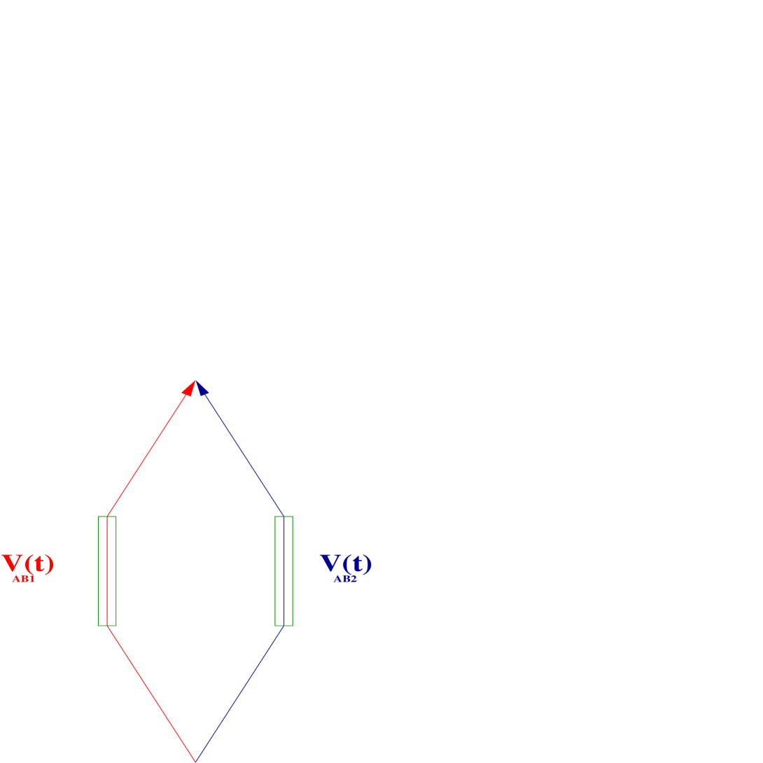
In quantum physics the situation is quite different. Quantum mechanics is a Hamiltonian theory were the dynamics of a charged particle in the presence of an electric field is governed by Schrödinger’s equation that can not be formulated directly in terms of the electric field. The introduction of an electric potential is required to define the Hamiltonian. Aharonov and Bohm observed [3] that this raises the possibility that a (time-dependent) electric potential could act on a charged particle even if it is constant in the region of space where the particle propagates, and they proposed an experiment to verify their theoretical prediction. See Figure 1. They advised to split a coherent electron beam into two parts and to let each one enter a long cylindrical metal tube. When each beam is well inside its tube, electric potentials are applied, in such a way that at any given time they are constant in the part of the tubes where each beam is propagating. The potentials are set to zero well before the beams leave the tubes. Finally, after the beams leave the tubes they are combined to interfere coherently. They claimed that as the potentials are constant in the region of the tubes where the beams propagate, the tubes act as a Faraday cage, and each beam picks up a phase given by the integral in time of its potential. If the potentials are different, so are the phases, and an interference fringe should be produced. This interference fringe is a purely quantum mechanical phenomenon, because on this experiment the beams are in a time-varying potential without ever being in an electric field, since the field does not penetrates far from the edges of the tubes, and it is only non-zero at times when the beams are well inside the tubes, far from the edges, what means that classically no force acts on the electron beams. This is the electric Aharonov-Bohm effect. In the same paper [3] they also proposed an experiment where a coherent electron beam is split into two beams and each one is allowed to pass, respectively, to the left and to the right of a magnetic field that is zero along the path of each beam. When the beams are behind the magnetic field they are combined to interfere. They predicted that an interference fringe will be observed that it is due to the action at a distance of the magnetic field and that it will depend on the circulation of the magnetic potential, what gives magnetic potentials a physical significance. This, of course, is impossible in classical physics. This is the magnetic Aharonov-Bohm effect. Note, however, that the existence of these interference fringes was previously predicted by Franz [10].

The experimental verification of the Aharonov-Bohm effects constitutes a test of the validity of the theory of quantum mechanics itself. For a review of the literature up to 1989 see [13] and [16]. In particular, in [16] there is a detailed discussion of the large controversy -involving over three hundred papers up to 1989- concerning the existence of the Aharonov-Bohm effect. For a recent update of this controversy see [7, 22, 25].

As mentioned in the abstract, the magnetic case has been extensively studied, but even the existence of the electric Aharonov-Bohm effect is questioned. Note that in the experiment [14] a steady-state version of the electric Aharonov-Bohm effect was tested and the expected phase shift was observed. However, as it was pointed out in [7], in the steady-state electric Aharonov-Bohm effect the electrons are subjected to a force and, for this reason, it is not considered to be a verification of the electric Aharonov-Bohm effect, where no forces act on the electrons.

As pointed out above, above, Aharonov and Bohm [3] proposed an Ansatz for the solution to the Schrödinger equation in regions where there is a time-dependent electric potential that is constant in space. It consists of multiplying the free evolution by a phase given by the integral in time of the potential. As the Aharonov-Bohm Ansatz predicts an interference fringe between the different parts of a coherent beam that are subjected to different potentials, the issue of the existence of the electric Aharonov-Bohm effect can be summarized in a single mathematical question: is the Aharonov-Bohm Ansatz a good approximation to the exact solution to the Schrödinger equation, under the conditions of the experiment proposed by Aharonov and Bohm. This is the question that we address in this paper.

Let us consider the case of one electron beam and one tube, $K$, or, equivalently, the part of the electron beam that travels inside one of the tubes, after splitting the original beam into two. For the Aharonov-Bohm Ansatz to be valid it is necessary that, to a good approximation, the electron does not interact with $K$, because if it hits $K$ it will be reflected and the solution can not be the free evolution multiplied by a phase. This is true no matter how big the velocity is. For this reason we consider a general class of incoming asymptotic states with the property that under the free classical evolution they do not hit $K$. The intuition is that for high velocity the exact quantum mechanical evolution is close to the free quantum mechanical evolution and that as the free quantum mechanical evolution is concentrated on the classical trajectories, we can expect that, in the leading order for high velocity, we do not see the influence of $K$ and that only the influence of electric potential inside $K$ shows up in the form of a phase, as predicted by the Aharonov-Bohm Ansatz.

We prove in this paper that the exact solution to the Schrödinger equation is given by the Aharonov-Bohm Ansatz, up to an error bound in norm that is uniform in time and that decays as a constant divided by the velocity $v$. In our bound the direction of the velocity is kept fixed, along the axis of the tube, as it absolute value goes to infinite.

We study this problem in ${\mathbb{R}}^{n},n\geq 2,$ because the proofs are the same for all $n\geq 2$, but of course, the physical case is $n=3$.

Let us denote $\mathbf{p}:=-i\nabla$. The Schrödinger equation for an electron in $\Lambda:={\mathbb{R}}^{n}\setminus K$, with electric potential ${\mathbf{V}}(t,x)$ is given by

$$i\hbar\frac{\partial}{\partial t}\phi=\frac{1}{2M}{\mathbf{P}}^{2}\phi+q\,\mathbf{V}(t,x)\phi,$$ (1.1)

where $\hbar$ is Planck’s constant, ${\mathbf{P}}:=\hbar\mathbf{p}$ is the momentum operator, and $M$ and $q$ are, respectively, the mass and the charge of the electron.

Suppose that $K$ is centered at the origin, $x=0$, and that its axis is along the vertical coordinate, $x_{n}$. Furthermore, assume that the velocity of the electron is along $x_{n}$ and that at time zero it is localized well inside $K$, in a neighborhood of the origin. Let $\mathbf{V}_{AB}$ be the electric potential in the experiment proposed by Aharonov and Bohm. $\mathbf{V}_{AB}$ is zero before the electron enters $K$, then it grows in time when the electron is well inside $K$, and finally if falls back to zero before the electron comes near the other edge of $K$. Note that the electron is inside the tube during a time interval, around zero, of the order $1/v$. Hence, $\mathbf{V}_{AB}$ is different from zero only during a time interval of the order $1/v$. Since as $v$ increases the time that $\mathbf{V}_{AB}$ acts on the electron decreases as $1/v$, in order that its effect does not disappears for large $v$ it is necessary that the strength of $\mathbf{V}_{AB}$ increases with the velocity $v$. For this reason we take $\mathbf{V}_{AB}$ as follows,

$$\mathbf{V}_{AB}(vt,x):=v\,\mathbf{Q}(vt,x).$$ (1.2)

We denote by $K_{0}$ the hole of $K$ . Let $B_{R}$ denote the open ball of center zero and radius $R$. We assume that for some $L_{1}>L_{0}>0$, such that $B_{L_{1}}\subset K_{0}$, we have that $\mathbf{Q}(z,x)=0,|z|\geq L_{0}$ and that for $|z|<L_{0},\,\,\mathbf{Q}(z,x)=\mathbf{Q}_{0}(z)$ for $x\in B_{L_{1}}$, where $\mathbf{Q}_{0}(z)$ is a continuously differentiable function that vanishes for $|z|\geq L_{0}$. Note that $z=vt$ is the distance along the classical trajectory of an electron that propagates with velocity $\mathbf{v}$.

Since high-velocity estimates of solutions to Schrödinger equations are of independent interest, we consider a situation that goes beyond the electric Aharonov-Bohm effect and assume that the electric potential is of the form,

$$\mathbf{V}(x,t):=\mathbf{V}_{AB}(vt,x)+\mathbf{V}_{0}(t,x).$$ (1.3)

where $\mathbf{V}_{0}$ is a potential that is uniformly bounded on the velocity. As we prove below $\mathbf{V}_{0}$ gives no contribution to the leading order for high velocity, and then, on this regime, it plays no role in the electric Aharonov-Bohm effect.

The free Hamiltonian $\mathbf{H}_{0}$ is given by

$$\mathbf{H}_{0}:=\frac{1}{2M}\,\mathbf{P}^{2}.$$

The incoming free electron beam with velocity $\mathbf{v}$ is given by

$$\psi_{\mathbf{v},0}=e^{-i\frac{t}{\hbar}\,\mathbf{H}_{0}}\,\varphi_{\mathbf{v}},$$

where

$$\varphi_{\mathbf{v}}=e^{i\frac{M}{\hbar}\mathbf{v}\cdot x}\,\varphi.$$

We designate by $\Lambda$ the complement of the tube: $\Lambda:={\mathbb{R}}^{n}\setminus K$. For any $\mathbf{v}\neq 0$ we denote,

$$\Lambda_{\hat{\mathbf{v}}}:=\{x\in\Lambda:x+\tau\hat{\mathbf{v}}\in\Lambda,\,\forall\tau\in{\mathbb{R}}\},$$

where $\hat{\mathbf{v}}:=\mathbf{v}/|\mathbf{v}|$. We show in Subsection 3.1 that the incoming free electron beams $\psi_{\mathbf{v},0}$ with support $\varphi\subset\Lambda_{\mathbf{v}}$ have negligible interaction with the cylinder $K$ for large velocities if the wave packet spreading is neglected. In fact, it is only for this type of incoming electron beams that we can expect that the Aharonov-Bohm Ansatz is a good approximation to the exact solution for large velocities.

We denote,

$$F_{-}(t):=v\int_{-\infty}^{t}\,\frac{q}{\hbar}\mathbf{Q}_{0}(vs)\,ds.$$

The Aharonov-Bohm Ansatz is given by,

$$\psi_{AB,\mathbf{v}}(t,x):=e^{-i\,v\int_{-\infty}^{t}\,\frac{q}{\hbar}\mathbf{Q}_{0}(vs)\,ds}\,e^{-i\frac{t}{\hbar}\,\mathbf{H}_{0}}\,\varphi_{\mathbf{v}}.$$

The unique solution to the Schrödinger equation (1.1) that behaves as the free incoming electron beam, $\psi_{\mathbf{v},0}$, as $t\rightarrow-\infty$ is given by

$$\psi_{\mathbf{v}}:=U(t,0)\,W_{-}\,\varphi_{\mathbf{v}},$$

where $U(t,0)$ is the propagator for (1.1) and $W_{-}$ is a wave operator. See Subsection 2.3 and equations (2.31, 3.3, 3.4).

By Theorem 3.2 in Subsection 3.3, for any $\mathbf{v}\in{\mathbb{R}}^{n}\setminus 0$ such that $B_{L_{1}}\subset\Lambda_{\mathbf{v}}$ and for any $0<R<L_{1}-L_{0}$ there is a constant $C$ such that,

$$\left\|U(t,0)\,\,\psi_{\mathbf{v}}-\psi_{AB,\mathbf{v}}\right\|\leq\,C\,\|\varphi\|_{\mathcal{H}_{2}({\mathbb{R}}^{n})}\,\,{\mathcal{E}}(v),$$

for all $\varphi$ in the Sobolev space $\mathcal{H}_{2}({\mathbb{R}}^{n})$ with support contained in $B_{R}$, and where the error ${\mathcal{E}}(v)$ is given by,

$${\mathcal{E}}(v):=\left\{\begin{array}[]{c}\displaystyle\frac{1}{v^{\rho}},\quad 0<\rho<1,\\ \\ \displaystyle\frac{|\ln v|}{v},\quad\rho=1,\\ \\ \displaystyle\frac{1}{v},\quad\rho>1,\end{array}\right.$$ (1.4)

for $v>0$ and where $\rho$ gives the decay rate of $\mathbf{V}_{0}$ as $|x|\rightarrow\infty$. See equation (2.8).

Note that $\mathcal{E}=1/v$ if $V_{0}$ decays as a short-range potential at infinite. Actually, for the purpose of the Aharonov-Bohm effect we can take $V_{0}=0$. We give a precise definition of $K$ in Subsection 2.1 and in Subsection 2.2 we state our conditions in the electric potential $\mathbf{V}$.

Let us consider the experiment proposed by Aharonov and Bohm [3] in three dimensions with one cylinder with axis along the vertical coordinate $x_{3}$ and let us take $\mathbf{v}$ directed along $x_{3}$. We consider an incident coherent electron beam that we split into two parts. One travels inside the tube where it is influenced by the Aharonov-Bohm potential and the other, that is the reference beam, travels outside the tube where the Aharonov-Bohm potential is zero. Finally, both parts are brought together behind the tube and are allowed to interfere. We can equivalently consider that both beams travel inside the tube, one with the Aharonov-Bohm potential and the other without it. For high velocity $\psi_{\mathbf{v}}$ is well approximated by $\psi_{AB,\mathbf{v}}$. Furthermore, behind the tube,

$$\psi_{AB,\mathbf{v}}=\,e^{-i\frac{q}{\hbar}\mathbf{\Phi}}\,e^{-i\frac{t}{\hbar}\,\mathbf{H}_{0}}\,\varphi_{\mathbf{v}},\,\hbox{\rm for}\,t\geq L_{0}/v,\,\hbox{\rm or}\,z=vt\geq L_{0}$$

where,

$$\mathbf{\Phi}:=\int_{-L_{0}}^{L_{0}}\,\mathbf{Q}_{0}(z)\,dz.$$

The reference beam is given by,

$$e^{-i\frac{t}{\hbar}\,\mathbf{H}_{0}}\,\varphi_{\mathbf{v}}.$$

We see that the beam that travels inside the tube with the Aharonov-Bohm potential, and the reference beam show precisely the difference in phase predicted by Aharonov and Bohm [3]. Our results prove, for the first time, that quantum mechanics rigorously predicts the existence of the electric Aharonov-Bohm effect for high velocity, and under appropriate conditions that we provide in Theorem 3.2. Our results settle the theoretical issues. It would be quite interesting if the existence of this fundamental phenomenon could be experimentally verified.

The results of this paper, as well as those of [4, 5, 6, 28], are proven using the method to estimate the high-velocity behaviour of solutions to the Schrödinger equation and of the scattering operator that was introduced in [9], and was applied to time-dependent potentials in all space in [27].

The paper is organized as follows. In Section 2 we state preliminary results that we need. In Section 3 we obtain our estimates for the leading order at high velocity of the exact solution to the Schrödinger equation and we use them to prove that quantum mechanics rigorously predicts the existence of the electric Aharonov-Bohm effect under conditions that we provide. The main result is Theorem 3.2 where we obtain our high-velocity estimates for the exact solution to the Schrödinger equation that give precise conditions for the validity of the Aharonov-Bohm Ansatz, with an error bound in norm, given by ${\mathcal{E}}(v)$, that is uniform in time. In Theorems 3.3 and 3.4 we obtain high velocity estimates for the wave and the scattering operators that prove that these operators act as multiplication by a constant phase given by integrals in time of the Aharonov-Bohm potential inside the tube, modulo an error that is uniform in time, and that as before, is given ${\mathcal{E}}(v)$.

Finally some words about our notations and definitions. We denote by $C$ any finite positive constant whose value is not specified. For any $x\in{\mathbb{R}}^{n},x\neq 0$, we denote, $\hat{x}:=x/|x|$. For any $\mathbf{v}\in{\mathbb{R}}^{n}$ we designate, $v:=|\mathbf{v}|$. As mentioned above, by $B_{R}$ we denote the open ball of center 00 and radius $R$. For any set $O$ we denote by $\chi_{O}(x)$ the characteristic function of $O$ and by $F(x\in O)$ the operator of multiplication by the characteristic function of $O$. By $\|\cdot\|$ we denote the norm in $L^{2}(\Lambda)$ where, as above, $\Lambda:={\mathbb{R}}^{n}\setminus K$. The norm of $L^{2}({\mathbb{R}}^{n})$ is denoted by $\|\cdot\|_{\displaystyle L^{2}({\mathbb{R}}^{n})}$. For any open set, $O$, we denote by $\mathcal{H}_{s}(O),\,s=1,2,\cdots$ the Sobolev spaces [1] and by $\mathcal{H}_{s,0}(O)$ the closure of $C^{\infty}_{0}(O)$ in the norm of $\mathcal{H}_{s}(O)$. By $\mathcal{B}(O)$ we designate the Banach space of all bounded operators on $L^{2}(O)$. We denote by $\|\cdot\|_{\displaystyle\mathcal{B}({\mathbb{R}}^{n})}$ the operator norm in $L^{2}({\mathbb{R}}^{n})$.

We define the Fourier transform as a unitary operator on $L^{2}({\mathbb{R}}^{n})$ as follows,

$$\hat{\phi}(p):=F\phi(p):=\frac{1}{(2\pi)^{n/2}}\int_{{\mathbb{R}}^{n}}e^{-ip\cdot x}\phi(x)\,dx.$$

We define functions of the operator $\mathbf{p}:=-i\nabla$ by Fourier transform,

$$f(\mathbf{p})\phi:=F^{\ast}f(p)F\phi,\,D(f(\mathbf{p})):=\{\phi\in L^{2}({\mathbb{R}}^{n}):f(p)\,\hat{\phi}(p)\in L^{2}({\mathbb{R}}^{n})\},$$

for every measurable function $f$.

Let us mention some related rigorous results on the Aharonov-Bohm effect. For further references see [4, 5, 6], and [28]. In [11], a semi-classical analysis of the Aharonov-Bohm effect in bound-states in two dimensions is given. The papers [19], [20], [29], and [30] study the scattering matrix for potentials of Aharonov-Bohm type in the whole space.

2 Preliminary Results

We consider a non-relativistic particle, like an electron, that propagates outside a bounded metallic tube, $K$, in ${\mathbb{R}}^{n},n\geq 2$, with its axis along the vertical direction. In the propagation domain $\Lambda:={\mathbb{R}}^{n}\setminus K$ there is a time-dependent electric potential as in (1.3). To simplify the notation we multiply both sides of Schrödinger’s equation (1.1) by $\frac{1}{\hbar}$ and we write it as follows

$$i\frac{\partial}{\partial t}\phi=\frac{1}{2m}\mathbf{p}^{2}\phi+V\phi,$$ (2.1)

with $m:=M/\hbar$ and

$$V:=\frac{q}{\hbar}\mathbf{V}=V_{AB}(vt,x)+V_{0}(t,x),$$

where,

$$V_{AB}(vt,x):=\frac{q}{\hbar}\,{\mathbf{V}}_{AB}(vt,x)=vQ(vt,x),$$

with

$$Q(vt,x):=\frac{q}{\hbar}\,{\mathbf{Q}}(vt,x),$$

and

$$V_{0}(t,x):=\frac{q}{\hbar}\,{\mathbf{V}}_{0}(t,x).$$

2.1 The Tube $K$

For any $x=(x_{1},x_{2},\cdots,x_{n})\in{\mathbb{R}}^{n}$ we denote by $\overline{x}:=(x_{1},x_{2},\cdots,x_{n-1})$. Let $D_{1},D_{2}\subset{\mathbb{R}}^{n-1}$ be bounded open sets with $D_{1}\subset D_{2}$ and let $L>0$. The metallic tube, $K$, is the set

$$K:=\left\{x\in{\mathbb{R}}^{n}:\overline{x}\in\overline{D_{2}}\setminus D_{1},|x_{n}|\leq L/2\right\}.$$ (2.2)

For example, $K$ can be a cylindrical tube with with $D_{1}$ and $D_{2}$ balls in $n\geq 4$ or discs in the case $n=3$. The hole of the tube is the set,

$$K_{0}:=\left\{x\in\Lambda:\overline{x}\in D_{1},|x_{n}|\leq L/2\right\}.$$ (2.3)

2.2 The Electric Potential

The electric potential $V(t,x)$ is a real -valued function defined on $\Lambda$. In the following assumptions we summarize the conditions on $V(t,x)$ that we need.

We denote by $\Delta$ the self-adjoint realization of the Laplacian in $L^{2}({\mathbb{R}}^{n})$ with domain $\mathcal{H}_{2}({\mathbb{R}}^{n})$. We say that the operator of multiplication by a real valued function $f$ defined in $\Lambda$ is $\Delta$- bounded with relative bound zero if the extension of $f$ to ${\mathbb{R}}^{n}$ by zero is $\Delta-$ bounded with relative bound zero [12]. Using a extension operator from $\mathcal{H}_{2}(\Lambda)$ to $H_{2}({\mathbb{R}}^{n})$ [26] we prove that this is equivalent to require that $f$ is relatively bounded from $\mathcal{H}_{2}(\Lambda)$ into $L^{2}(\Lambda)$ with relative bound zero.

We always assume that the electric potential $V(t,x)$ satisfies the following assumptions.

$$V(t,x):=V_{AB}(vt,x)+V_{0}(t,x),$$ (2.4)

where the Aharonov-Bohm potential is given by,

$$V_{AB}(z,x):=v\,Q(z,x)$$ (2.5)

with $Q(z,x)=0$ for $x\in\Lambda\setminus K_{0}$ and for each fixed $x,\,Q(z,x)$ is continuously differentiable in $z$ and

$$\left|Q(z,x)\right|+\left|\frac{\partial}{\partial z}Q(z,x)\right|\leq C,$$ (2.6)

for some constant $C$. Furthermore, for each $t\in{\mathbb{R}}$ the operator of multiplication by the function $V_{0}(t,x)$ is $\Delta$-bounded with relative bound zero and the operator valued function

$$t\rightarrow V_{0}(t,x)\left(-\Delta+1\right)^{-1},$$ (2.7)

is continuously differentiable in $t\in{\mathbb{R}}$, with values in ${\mathcal{B}}({\mathbb{R}}^{n})$. Moreover, there are $L_{1}>L_{0}>0$ such that $B_{L_{1}}\subset K_{0}$ and $Q(z,x)=0,|z|\geq L_{0}$. Furthermore, for $|z|<L_{0},\,\,Q(z,x)=Q_{0}(z)$ for $x\in B_{L_{1}}$, where $Q_{0}(z)$ is a continuously differentiable function that vanishes for $|z|\geq L_{0}$. Note that $z=vt$ is the distance along the classical trajectory of an electron that propagates with velocity $\mathbf{v}$.

Furthermore, we assume that,

$$\left\|V_{0}(t,x)\left(-\Delta+1\right)^{-1}F(|x|\geq r)\right\|_{\mathcal{B}({\mathbb{R}}^{n})}\leq C(1+|t|)^{\mu}\,(1+r)^{-\rho},\quad r\geq 0,$$ (2.8)

where $\rho>0,\mu\in{\mathbb{R}},$ and $\rho-\mu>1$.

Remark that condition (2.8 is equivalent to the following assumption [18]

$$\left\|V_{0}(t,x)F(|x|\geq r)\left(-\Delta+1\right)^{-1}\right\|_{\mathcal{B}({\mathbb{R}}^{n})}\leq C(1+|t|)^{\mu}\,(1+r)^{-\rho},\quad r\geq 0.$$ (2.9)

Condition (2.9) has a clear intuitive meaning. It is an assumption on the decay of $V_{0}$ at infinite. However, in the proofs below we use the equivalent statement (2.8) because it is technically more convenient.

Note that when $\mu>0$ the potential $V_{0}(t,x)$ can grow in time. The physical reason for this is that, as in this case $V_{0}(t,x)$ goes to zero fast as $|x|\rightarrow\infty$, in the high-velocity limit the electron leaves the interacting region, where $V_{0}(t,x)$ is strong, in a very small time, and then, the grow in time of $V_{0}(t,x)$ does not affects the trajectory of the electron. When $\mu<0$, $V_{0}(t,x)$ can go to zero slowly as $|x|\rightarrow\infty$, but this is compensated by the fact that it goes to zero as time $|t|\rightarrow\infty$. Note that along the classical trajectory, $x=\mathbf{v}t,V_{0}(t,\mathbf{v}t)$ decays as $1/t^{\rho-\mu}$ with $\rho-\mu>1$, and hence, the effect of $V_{0}(t,x)$ is effectively of short-range, and, as we will see, the interacting evolution is well approximated by the free evolution, on spite of the fact that for each fixed time $V_{0}(t,x)$ can decay slowly as $|x|\rightarrow\infty$.

The electron is inside the tube during a time interval, around zero, of the order $1/v$. Hence, $V_{AB}$ is different from zero only during a time interval of the order $1/v$. Since as $v$ increases the time that $V_{AB}$ acts on the electron decreases as $1/v$, in order that its effect does not disappear for large $v$, it is necessary that the strength of $V_{AB}$ increases with the velocity $v$. Finally, note that $V(t,x)$ depends on $v$ through $V_{AB}$. To simplify the notation we do not make explicit this dependence on $v$.

Sufficient conditions for a multiplication by a function operator, $f$, to be $\Delta$- bounded with relative bound zero are well known. For example [17], for $n=3$, this is true if $f\in L^{2}({\mathbb{R}}^{3})$ and for $n\geq 4$ if $f\in L^{p}({\mathbb{R}}^{n})$ with $p>n/2$. The function in (2.7) is continuously differentiable, for example, if $t\rightarrow V_{0}(t,x)$ is a continuously differentiable function with values in $L^{2}({\mathbb{R}}^{3}$ for $n=3$ and in $L^{p}({\mathbb{R}}^{n})$ with $p>n/2$ for $n\geq 4$. Obviously, we can replace $L^{2}({\mathbb{R}}^{3})$ by $L^{\infty}({\mathbb{R}}^{3})$ and $L^{p}({\mathbb{R}}^{n})$ by $L^{\infty}({\mathbb{R}}^{n})$ in the conditions above, or by the sum of potentials of this type. For more general sufficient conditions see [21].

2.3 The Unitary Propagator

We define the unperturbed quadratic form,

$$h_{0}(\phi,\psi):=\frac{1}{2m}(\mathbf{p}\phi,\mathbf{p}\psi),\,D(h_{0}):=\mathcal{H}_{1,0}(\Lambda).$$

The associated positive operator in $L^{2}(\Lambda)$ [12], [17] is

$$\frac{-1}{2m}\Delta_{D},$$

where $\Delta_{D}$ is the Laplacian with Dirichlet boundary condition on $\partial\Lambda$. Note that the functions in $\mathcal{H}_{1,0}(O)$ vanish in trace sense in the boundary of $O$. By elliptic regularity [2], $D(\Delta_{D})=\mathcal{H}_{2}(\Lambda)\cap\mathcal{H}_{1,0}(\Lambda)$.

We define the perturbed Hamiltonian as follows,

$$H(t):=\frac{-1}{2m}\Delta_{D}+V(t,x),\quad t\in{\mathbb{R}},$$ (2.10)

with domain, $D(H(t)):=D(\Delta_{D})=\mathcal{H}_{2}(\Lambda)\cap\mathcal{H}_{1,0}(\Lambda)$ independent of $t$. Since $V(t,x)$ is $\Delta-$ bounded with relative bound zero it follows from Kato-Rellich’s theorem [12, 17] that $H(t)$ is self-adjoint and bounded below in $L^{2}(\Lambda)$. Note that $H(t)$ is the physical perturbed Hamiltonian divided by $\hbar$. This is so, because we obtained equation (2.1) multiplying both sides of the Schrödinger equation (1.1) by $\frac{1}{\hbar}$.

We define the Hamiltonian $H(t)$ in $L^{2}(\Lambda)$ with Dirichlet boundary condition at $\partial\Lambda$, i.e. $\phi=0$ for $x\in\partial\Lambda$. This is the standard boundary condition that corresponds to an impenetrable tube $K$. It implies that the probability that the electron is at the boundary of the tube is zero.

It follows from Theorem X.70 and from the proof of theorem X.71 of [17] that under our conditions there exists a unitary propagator $U(t,q),t,q\in{\mathbb{R}}$ such that:

  1. 1.

    $U(t,q),t,q\in{\mathbb{R}}$ is a two-parameter family of unitary operators on $L^{2}(\Lambda)$.

  2. 2.

    $U(t,q)\,U(q,r)=U(t,r),U(t,t)=I,\quad\forall\,t,q,r\in{\mathbb{R}}$.

  3. 3.

    $U(t,q)$ is jointly strongly continuous in $t,q\in{\mathbb{R}}$.

  4. 4.

    $U(t,q)D(\Delta_{D})\subset D(\Delta_{D}),\,\forall\,\,t,q\in{\mathbb{R}}$ and $\forall\phi\in D(\Delta_{D})$

    $$i\frac{\partial}{\partial t}\,U(t,q)\phi=H(t)\,U(t,q)\phi,\quad i\frac{\partial}{\partial q}\,U(t,q)\phi=-U(t,q)\,H(q)\phi,\quad t,q\in{\mathbb{R}}.$$

The unitary propagator gives us the unique solution to Schrödinger’s equation (2.1) with initial data $\phi\in D(\Delta_{D})$ at $t=q$ and with Dirichlet boundary condition at $\partial\Lambda$.

2.4 Propagation Estimates

The free Hamiltonian is the self-adjoint operator in $L^{2}({\mathbb{R}}^{n})$,

$$H_{0}:=-\frac{1}{2m}\Delta$$ (2.11)

where $\Delta$ is the self-adjoint realization of the Laplacian with domain $\mathcal{H}_{2}({\mathbb{R}}^{n})$. The solution to the free Schrödinger equation,

$$i\frac{\partial}{\partial t}\phi(t,x)=H_{0}\phi(t,x),x\in{\mathbb{R}}^{n},t\in{\mathbb{R}},\phi(0,x)=\phi_{0}\in D(H_{0}),$$ (2.12)

is given by

$$\phi(t,x)=e^{-itH_{0}}\,\phi_{0}.$$ (2.13)

It follows by Fourier transform that under translation in configuration or momentum space generated, respectively, by $\mathbf{p}$ and $x$ we obtain

$$e^{i\mathbf{p}\cdot\mathbf{v}t}\,f(x)\,e^{-i\mathbf{p}\cdot\mathbf{v}t}=f(x+\mathbf{v}t),$$ (2.14)
$$e^{-im\mathbf{v}\cdot x}\,f(\mathbf{p})\,e^{im\mathbf{v}\cdot x}=f(\mathbf{p}+m\mathbf{v}),$$ (2.15)

and, in particular,

$$e^{-im\mathbf{v}\cdot x}\,e^{-itH_{0}}\,e^{im\mathbf{v}\cdot x}=e^{-imv^{2}t/2}\,e^{-i\mathbf{p}\cdot\mathbf{v}t}\,e^{-itH_{0}}.$$ (2.16)

We need the following lemma from [28].

LEMMA 2.1.

For any $f\in C^{\infty}_{0}(B_{m\eta})$ for some $\eta>0$ and any $j=1,2,\cdots$ there is a constant $C_{j}$ such that the following estimate holds

$$\left\|F(x\in\tilde{M})\,e^{-itH_{0}}\,f\left(\frac{\mathbf{p}-m\tilde{\mathbf{v}}}{\tilde{v}}\right)\,F(x\in M)\right\|_{{\mathcal{B}}({\mathbb{R}}^{n})}\leq C_{j}\,\left(1+\lambda\tilde{v}+\eta\tilde{v}^{2}|t|\right)^{-j},$$ (2.17)

for any $\tilde{\mathbf{v}}\in{\mathbb{R}}^{n}\setminus 0,\tilde{v}:=|\tilde{\mathbf{v}}|,t\in{\mathbb{R}}$, and any measurable sets $\tilde{M},M$ in ${\mathbb{R}}^{n}$ such that $\lambda:=\hbox{\rm dist}\,\left(\tilde{M},M+\tilde{\mathbf{v}}t\right)-\eta\tilde{v}|t|\geq 0$.

Proof: This is the particular case of Lemma 2.1 of [28] with $\rho=1$ and $\tilde{v}=|\tilde{\mathbf{v}}|$. Note that the proof in $n$ dimensions is the same as the one in two dimensions given in [28].

LEMMA 2.2.

For any $f\in C^{\infty}_{0}(B_{m\eta})$ for some $0<\eta<1/8$, and for any $j=1,2,\cdots$ there is a constant $C_{j}$ such that

$$\left\|F\left(|x-\tilde{\mathbf{v}}t|>\frac{|\tilde{v}t|}{4}\right)e^{-itH_{0}}\,f\left(\displaystyle\frac{\mathbf{p}-m\tilde{\mathbf{v}}}{\tilde{v}}\right)\,F\left(|x|\leq|\tilde{v}t|/8\right)\right\|_{{\mathcal{B}}({\mathbb{R}}^{n})}\leq C_{j}(1+|\tilde{v}^{2}t|)^{-j},$$ (2.18)

for $\tilde{v}:=|\tilde{\mathbf{v}}|>0$.

Proof: The lemma follows from Lemma 2.1 with $\tilde{M}=\{|x-\tilde{\mathbf{v}}t|>|\tilde{v}t|/4\}$ and $M=\{|x|\leq|\tilde{v}t|/8\}$. Observe that $\lambda:=\hbox{\rm dist}\,\left(\tilde{M},M+\tilde{\mathbf{v}}t\right)-\eta\tilde{v}|t|\geq|\tilde{v}t|(1/8-\eta)$.

$\Box$

Recall that ${\mathcal{E}}(v)$ was defined in (1.4).

LEMMA 2.3.

Let $f\in C^{\infty}_{0}(B_{m\eta}),0<\eta<1/8$. Suppose that $\mathcal{V}(t,x)$ satisfies (2.8) or, equivalently, (2.9). Then, for any compact set $D\subset{\mathbb{R}}^{n}$ and any $\tilde{v}_{0}>0$, there is a constant $C$ such that for all $\tilde{v}\geq\tilde{v}_{0}$,

$$\int_{-\infty}^{\infty}\,dt\,\|\mathcal{V}(t,x)e^{-itH_{0}}\,e^{im\tilde{\mathbf{v}}\cdot x}\,f\left(\displaystyle\frac{\mathbf{p}}{\tilde{v}}\right)\phi\|_{L^{2}({\mathbb{R}}^{n})}\leq C\,\|\phi\|_{\mathcal{H}_{2}({\mathbb{R}}^{n})}\,{\mathcal{E}}(\tilde{v}),$$ (2.19)

for all $\phi\in\mathcal{H}_{2}({\mathbb{R}}^{n})$ with support in $D$.

Furthermore , suppose that $\mathcal{V}(t,x)$ satisfies,

$$\left\|\mathcal{V}(t,x)F(|x|\geq r)\right\|_{\mathcal{B}({\mathbb{R}}^{n})}\leq C(1+|t|)^{\mu}\,(1+r)^{-\rho},\quad r\geq 0,$$ (2.20)

where $\rho>0,\,\mu\in{\mathbb{R}},$ and $\rho-\mu>1.$ Then, for any compact set $D\subset{\mathbb{R}}^{n}$ and any $\tilde{v}_{0}>0$, there is a constant $C$ such that for all $\tilde{v}\geq\tilde{v}_{0}$,

$$\int_{-\infty}^{\infty}\,dt\,\|\mathcal{V}(t,x)e^{-itH_{0}}\,e^{im\tilde{\mathbf{v}}\cdot x}\,f\left(\displaystyle\frac{\mathbf{p}}{\tilde{v}}\right)\phi\|_{L^{2}({\mathbb{R}}^{n})}\leq C\,\|\phi\|_{L^{2}({\mathbb{R}}^{n})}\,{\mathcal{E}}(\tilde{v}),$$ (2.21)

for all $\phi\in L^{2}({\mathbb{R}}^{n})$ with support in $D$.

Proof: It follows from (2.15) that,

$$\begin{array}[]{c}\mathcal{V}(t,x)e^{-itH_{0}}\,e^{im\tilde{\mathbf{v}}\cdot x}\,f\left(\displaystyle\frac{\mathbf{p}}{\tilde{v}}\right)\phi=e^{im\tilde{\mathbf{v}}\cdot x}\mathcal{V}(t,x)\,(-\Delta+1)^{-1}e^{-it(\mathbf{p}+m\tilde{\mathbf{v}})^{2}/2m}f\left(\displaystyle\frac{\mathbf{p}}{\tilde{v}}\right)\,(-\Delta+1)\,\phi=\\ \\ e^{im\tilde{\mathbf{v}}\cdot x}\mathcal{V}(t,x)\,(-\Delta+1)^{-1}\,e^{-im\tilde{\mathbf{v}}\cdot x}\,e^{-itH_{0}}\,f\left(\displaystyle\frac{\mathbf{p}-m\tilde{\mathbf{v}}}{\tilde{v}}\right)\,e^{im\tilde{\mathbf{v}}\cdot x}\,(-\Delta+1)\,\phi.\end{array}$$ (2.22)

Then, we have that,

$$\left\|\mathcal{V}(t,x)e^{-itH_{0}}\,e^{im\tilde{\mathbf{v}}\cdot x}f\left(\displaystyle\frac{\mathbf{p}}{\tilde{v}}\right)\phi\right\|_{L^{2}({\mathbb{R}}^{n})}\leq I_{1}+I_{2}+I_{3},$$ (2.23)

where,

$$I_{1}:=\left\|\mathcal{V}(t,x)(-\Delta+1)^{-1}F\left(|x-\tilde{\mathbf{v}}t|>\frac{|\tilde{v}t|}{4}\right)e^{-itH_{0}}f\left(\displaystyle\frac{\mathbf{p}-m\tilde{\mathbf{v}}}{\tilde{v}}\right)\,F\left(|x|\leq|\tilde{v}t|/8\right)\right\|_{\mathcal{B}({\mathbb{R}}^{n})}\,\|\phi\|_{\mathcal{H}_{2}({\mathbb{R}}^{n})},$$ (2.24)
$$I_{2}:=C\,\left\|\mathcal{V}(t,x)(-\Delta+1)^{-1}\right\|_{\mathcal{B}({\mathbb{R}}^{n})}\,\|F\left(|x|>|\tilde{v}t|/8\right)(-\Delta+1)\phi\|_{L^{2}({\mathbb{R}}^{n})},$$ (2.25)
$$I_{3}:=C\left\|\mathcal{V}(t,x)(-\Delta+1)^{-1}F\left(|x-\tilde{\mathbf{v}}t|\leq\frac{|\tilde{v}t|}{4}\right)\right\|_{\mathcal{B}({\mathbb{R}}^{n})}\,\|\phi\|_{\mathcal{H}_{2}({\mathbb{R}}^{n})}.$$ (2.26)

By (2.8) with $r=0$ and (2.18),

$$I_{1}\leq\,C_{j}\,(1+\tilde{v}_{0}|\tilde{v}t|)^{-j}\,\|\phi\|_{\mathcal{H}_{2}({\mathbb{R}}^{n})},\quad j=1,2,\cdots.$$ (2.27)

Since $\phi$ has compact support in $D$,

$$\|F(|x|>|\tilde{v}t|/8)(-\Delta+1)\phi\|_{L^{2}({\mathbb{R}}^{n})}\leq C_{j}(1+|\tilde{v}t|)^{-j}\|(1+|x|)^{j}(\Delta+1)\phi\|_{L^{2}({\mathbb{R}}^{n})}\leq C_{j}\,(1+|\tilde{v}t|)^{-j}\,\|\phi\|_{\mathcal{H}_{2}({\mathbb{R}}^{n})},\quad j=1,2,\cdots.$$

Hence, by (2.8) with $r=0$,

$$I_{2}\leq\,C_{j}\,(1+|\tilde{v}t|)^{-j}\,\|\phi\|_{\mathcal{H}_{2}({\mathbb{R}}^{n})},\quad j=1,2,\cdots.$$ (2.28)

It follows from (2.27, 2.28) that

$$\int_{-\infty}^{\infty}\,dt\,(I_{1}+I_{2})\,\leq\,C\,\frac{1}{\tilde{v}}\,\int_{-\infty}^{\infty}\,dz\,(1+|z|)^{-2}\,\|\phi\|_{\mathcal{H}_{2}({\mathbb{R}}^{n})}=C\frac{1}{\tilde{v}}\,\|\phi\|_{\mathcal{H}_{2}({\mathbb{R}}^{n})}.$$ (2.29)

Furthermore, by (2.8)

$$\int_{-\infty}^{\infty}\,dt\,I_{3}\leq C\,\int_{-\infty}^{\infty}\,dt\,(1+|t|)^{\mu}\,(1+|\tilde{v}t|)^{-\rho}\,\|\phi\|_{\mathcal{H}_{2}({\mathbb{R}}^{n})}\,\leq C\,\|\phi\|_{\mathcal{H}_{2}({\mathbb{R}}^{n})}\,{\mathcal{E}}(\tilde{v}).$$ (2.30)

Equation (2.19) follows from (2.23, 2.29, 2.30). Finally, (2.21) is proven in the same way but, as in this case the regularization $(-\Delta+1)^{-1}$ is not needed, we obtain the norm of $\varphi$ in $L^{2}({\mathbb{R}}^{n})$.

2.5 The Wave and Scattering Operators

Let $J$ be the identification operator from $L^{2}({\mathbb{R}}^{n})$ onto $L^{2}(\Lambda)$ given by multiplication by the characteristic function of $\Lambda$. The wave operators are defined as follows,

$$W_{\pm}:=\hbox{\rm s-}\lim_{t\rightarrow\pm\infty}U(0,t)\,J\,e^{-itH_{0}},$$ (2.31)

provided that the strong limits exist. It follows from the Rellich local compactness theorem [1, 18] that $J$ can be replaced by the operator of multiplication by any function $\chi\in C^{\infty}({\mathbb{R}}^{n})$ that satisfies $\chi(x)=0$ in a bounded neighborhood of $K$ and $\chi(x)=1$ for $x$ in the complement of another bounded neighborhood of $K$,

$$W_{\pm}:=\hbox{\rm s-}\lim_{t\rightarrow\pm\infty}U(0,t)\,\chi\,e^{-itH_{0}}.$$ (2.32)
LEMMA 2.4.

The wave operators $W_{\pm}$ exist, they are partially isometric with initial subspace $L^{2}({\mathbb{R}}^{n})$ and they satisfy the intertwining relations,

$$U(t,0)\,W_{\pm}=W_{\pm}\,e^{-itH_{0}}.$$ (2.33)

Proof: It is enough to prove the existence of the $W_{\pm}$ for all functions of the type,

$$e^{im\tilde{\mathbf{v}}\cdot x}f\left(\frac{\mathbf{p}}{\tilde{v}}\right)\phi,$$

with $\phi\in\mathcal{H}_{2}({\mathbb{R}}^{n})$ of compact support and $f\in C^{\infty}_{0}(B_{m\eta})$ where $\eta<1/8$ because the set of all linear combinations of these functions is dense in $L^{2}({\mathbb{R}}^{n})$.

By equation (2.32) and Duhamel’s formula,

$$W_{\pm}\,e^{im\tilde{\mathbf{v}}\cdot x}f\left(\frac{\mathbf{p}}{\tilde{v}}\right)\phi=e^{im\tilde{\mathbf{v}}\cdot x}f\left(\frac{\mathbf{p}}{\tilde{v}}\right)\phi+i\int_{0}^{\pm\infty}\,dt\,U(0,t)\,\left[H(t)\,\chi(x)-\chi(x)\,H_{0}\right]\,e^{-itH_{0}}\,e^{im\tilde{\mathbf{v}}\cdot x}f\left(\frac{\mathbf{p}}{\tilde{v}}\right)\phi.$$ (2.34)

Since,

$$\left[H(t)\,\chi(x)-\chi(x)\,H_{0}\right]=V(t,x)-\frac{1}{2m}(\Delta\chi(x))-i\frac{1}{m}(\nabla\chi(x))\cdot\mathbf{p},$$

the integral in the right-hand side of (2.34) is absolutely convergent by Lemma 2.3. The fact that the $W_{\pm}$ are partially isometric with initial subspace $L^{2}({\mathbb{R}}^{n})$ follows from Rellich’s local compactness theorem [1, 18], and the intertwining relations (2.33) are immediate from the definition of $W_{\pm}$.

$\Box$

The scattering operator is defined as

$$S:=W_{+}^{\ast}\,W_{-}.$$ (2.35)

3 High-Velocity Estimates

3.1 High-Velocity Solutions to the Schrödinger Equation

At the time of emission, i.e., as $t\rightarrow-\infty$, the electron wave packet is far away from $K$ and it does not interact with it. Therefore, it can be parametrised with kinematical variables and it can be assumed that it follows the free evolution (2.13) of an asymptotic state, $\varphi_{\mathbf{v}}$, with velocity $\mathbf{v}$,

$$\psi_{\mathbf{v},0}:=e^{-itH_{0}}\,\varphi_{\mathbf{v}},$$ (3.1)

where

$$\varphi_{\mathbf{v}}:=e^{im\mathbf{v}\cdot x}\,\varphi,\quad\varphi\in L^{2}({\mathbb{R}}^{n}).$$ (3.2)

Note that in the momentum representation $e^{im\mathbf{v}\cdot x}$ is a translation operator by the vector $m\mathbf{v}$, what implies that in this representation the asymptotic state (3.2) is centered at the classical momentum $m\mathbf{v}$,

$$\hat{\varphi}_{\mathbf{v}}(p)=\hat{\varphi}(p-m\mathbf{v}).$$

The exact electron wave packet, $\psi_{\mathbf{v}}(x,t)$, satisfies the interacting Schrödinger equation (2.1) for all times and as $t\rightarrow-\infty$ it has to approach the incoming wave packet, i.e.,

$$\lim_{t\rightarrow-\infty}\left\|\psi_{\mathbf{v}}-J\psi_{\mathbf{v},0}\right\|=0.$$

This means that we have to solve the interacting Schrödinger equation (2.1) with initial conditions at minus infinity. This is accomplished by the wave operator $W_{-}$. In fact, we have that,

$$\psi_{\mathbf{v}}=U(t,0)\,W_{-}\,\varphi_{\mathbf{v}},$$ (3.3)

because, as $U(t,0)$ is unitary,

$$\lim_{t\rightarrow-\infty}\left\|U(t,0)\,W_{-}\,\varphi_{\mathbf{v}}-J\,e^{-itH_{0}}\varphi_{\mathbf{v}}\right\|=0.$$ (3.4)

We prove in the same way that

$$U(t,0)\,W_{+}\,\varphi_{\mathbf{v}}$$ (3.5)

is the unique solution to the Schrödinger equation such that

$$\lim_{t\rightarrow\infty}\left\|U(t,0)\,W_{+}\,\varphi_{\mathbf{v}}-J\,e^{-itH_{0}}\varphi_{\mathbf{v}}\right\|=0.$$

In order to isolate the electric Aharonov-Bohm effect we need to separate the effect of $K$ as a rigid body from that of the electric potential inside the hole $K_{0}$. For this purpose, we need asymptotic states that have negligible interaction with $K$ for all times. This is possible for large enough velocities.

For any $\mathbf{v}\neq 0$ we denote,

$$\Lambda_{\hat{\mathbf{v}}}:=\{x\in\Lambda:x+\tau\hat{\mathbf{v}}\in\Lambda,\,\forall\tau\in{\mathbb{R}}\}.$$ (3.6)

Let us consider asymptotic states (3.2) where $\varphi$ has compact support contained in $\Lambda_{\hat{\mathbf{v}}}$. For the discussion below it is better to parametrise the free evolution of $\varphi_{\mathbf{v}}$ by the distance along the classical trajectory, $z=vt$, rather than by the time $t$. It follows from (2.16) that at distance $z$ the state is given by,

$$e^{-i\frac{z}{v}H_{0}}\,\varphi_{\mathbf{v}}=e^{im\mathbf{v}\cdot x}\,e^{-i\frac{mzv}{2}}\,e^{-i\frac{z}{v}H_{0}}\,e^{-i\mathbf{p}\cdot z\hat{\mathbf{v}}}\varphi.$$ (3.7)

Observe that $e^{-i\mathbf{p}\cdot z\hat{\mathbf{v}}}$ is a translation in a straight line along the classical free evolution,

$$\left(e^{-i\mathbf{p}\cdot z\hat{\mathbf{v}}}\varphi\right)(x)=\varphi(x-z\hat{\mathbf{v}}).$$ (3.8)

The term $e^{-i\frac{z}{v}H_{0}}$ gives raise to the quantum-mechanical spreading of the wave packet. For high velocities this term is one order of magnitude smaller than the classical translation, and if we neglect it we get that,

$$(e^{-i\frac{z}{v}H_{0}}\,\varphi_{\mathbf{v}})(x)\approx e^{i\frac{mzv}{2}}\,\varphi_{\mathbf{v}}(x-z\hat{\mathbf{v}}),\,\,\hbox{\rm for large}\,\,v.$$ (3.9)

We see that, in this approximation, for high velocities our asymptotic state evolves along the classical trajectory, modulo the global phase factor $e^{i\frac{mzv}{2}}$ that plays no role. The key issue is that the support of our incoming wave packet remains in $\Lambda_{\mathbf{v}}$ for all distances, or for all times, and in consequence it has no interaction with $K$. We can expect that for high velocities the exact solution $\psi_{\mathbf{v}}$ (3.3) to the interacting Schrödinger equation (2.1) is close to the incoming wave packet $\psi_{\mathbf{v},0}$ and that, in consequence, it also has negligible interaction with $K$, provided, of course, that the support of $\varphi$ is contained in $\Lambda_{\mathbf{v}}$. Below we give rigorous ground for this heuristic picture proving that in the leading order $\psi_{\mathbf{v}}$ is not influenced by $K$ and that it only contains information on the electric potential inside $K_{0}$.

3.2 The Aharonov-Bohm Ansatz

Aharonov and Bohm [3] observed that in a region of space where there is a potential $V(t)$ that is independent of $x$ the solution to the Schrödinger equation (2.1) with $\phi(0)=\phi_{0}$ is given by,

$$e^{-i\,\int_{0}^{t}\,ds\,V(s)}\,e^{-itH_{0}}\,\phi_{0}.$$

We define,

$$F_{-}(t):=v\int_{-\infty}^{t}\,Q_{0}(vs)\,ds.$$ (3.10)

Note that,

$$\begin{array}[]{c}F_{-}(t)=0,\quad t\leq-L_{0}/v,\\ \\ F_{-}(t)=F(L_{0}/v)=\Phi,\quad t\geq L_{0}/v,\end{array}$$ (3.11)

where,

$$\Phi:=\int_{-L_{0}}^{L_{0}}\,Q_{0}(z).$$ (3.12)

We define the following approximate solution to the Schrödinger equation (2.1),

$$\psi_{AB,\mathbf{v}}(t,x):=e^{-iF_{-}(t)}\,e^{-itH_{0}}\,\varphi_{\mathbf{v}},$$ (3.13)

where $\mathbf{v}$ is such that $B_{L_{1}}\subset\Lambda_{\mathbf{v}}$. For example, we can take $\mathbf{v}$ along the vertical direction $x_{n}$ or slightly tilted with respect to $x_{n}$. Furthermore, we assume that $\hbox{\rm support}\,\varphi\subset B_{R}$ for some $R<L_{1}-L_{0}$. Suppose for the moment that $V_{0}=0$. For $t\leq-L_{0}/v$, $V_{AB}=0$ and then, (2.1) is just the free Schrödinger equation (2.12). But as for $t\leq-L_{0}/v,\,F_{-}(t)=0,\,\psi_{AB,\mathbf{v}}$ is also a solution to the free Schrödinger equation. Moreover, as $\hbox{\rm support}\,\varphi\subset B_{R}$, we have that according to the classical free evolution with velocity $\mathbf{v}$, for $|t|<L_{0}/v$ the electron is inside the ball $B_{R+L_{0}}\subset B_{L_{1}}$. But, since in $B_{L_{1}},\,V_{AB}=v\,Q_{0}(vt)$ we can expect that $\psi_{AB,\mathbf{v}}$ is a good approximation to the exact solution for $|t|<L_{0}/v$. Finally, as for $t\geq L_{0}/v,\,V_{AB}=0$ we can expect that

$$e^{-i(t-L_{0}/v)H_{0}}e^{-i\Phi}e^{-i(L_{0}/v)H_{0}}\varphi_{\mathbf{v}},$$

is a good approximation to the exact solution for $t\geq L_{0}/v$. But,

$$e^{-i(t-L_{0}/v)H_{0}}e^{-i\Phi}e^{-i(L_{0}/v)H_{0}}\varphi_{\mathbf{v}}=\psi_{AB,\mathbf{v}},\quad\hbox{\rm for}\,t\geq L/v.$$

Furthermore, as $V_{0}$ is uniformly bounded in $v$, we can expect that for high velocity it gives a contribution that does not appear in the leading order of the solution. These considerations motivate the introduction of the following Aharonov-Bohm Ansatz.

The Aharonov-Bohm Ansatz 3.1.

Let $\mathbf{v}\in{\mathbb{R}}^{n}\setminus 0$ be such that $B_{L_{1}}\subset\Lambda_{\mathbf{v}}$. Let $\varphi\in\mathcal{H}_{2}({\mathbb{R}}^{n})$ satisfy $\hbox{\rm support}\,\varphi\subset B_{R}$, where $0<R<L_{1}-L_{0}$. Let $\psi_{\mathbf{v}}:=U(t,0)\,W_{-}\,\varphi_{\mathbf{v}}$ be the solution to the Schrödinger equation that behaves like $\psi_{\mathbf{v},0}:=e^{-itH_{0}}\,\varphi_{\mathbf{v}}$ as time goes to minus infinite. Then,

$$\psi_{\mathbf{v}}\approx\psi_{AB,\mathbf{v}}(t,x):=e^{-iF_{-}(t)}\,e^{-itH_{0}}\,\varphi_{\mathbf{v}},$$ (3.14)

for large velocity, $v:=|\mathbf{v}|$, and uniformly in time.

3.3 Uniform Estimates for the Exact solution to the Schrödinger Equation

In this subsection we estimate the high-velocity solutions to the Schrödinger equation.

Let $g\in C^{\infty}_{0}({\mathbb{R}}^{n})$ satisfy, $g(p)=1,|p|\leq m/32$ and $g(p)=0,|p|\geq\frac{m}{16}$. We denote,

$$\tilde{\varphi}:=g(\mathbf{p}/v)\,\varphi,\quad v>0.$$ (3.15)

By Fourier transform we prove that,

$$\left\|\tilde{\varphi}-\varphi\right\|_{L^{2}({\mathbb{R}}^{n})}\leq\frac{C}{1+v^{2}}\,\|\varphi\|_{\mathcal{H}_{2}({\mathbb{R}}^{n})}.$$ (3.16)

We define,

$$F_{+}(t):=v\int_{t}^{\infty}\,Q_{0}(vs)\,ds.$$ (3.17)

Note that,

$$\begin{array}[]{c}F_{+}(t)=0,\quad t\geq L_{0}/v,\\ \\ F_{+}(t)=F_{+}(-L_{0}/v)=\Phi,\quad t\leq-L_{0}/v,\end{array}$$ (3.18)

where $\Phi$ is defined in (3.12)

The next theorem is our main result where we give our high-velocity estimates, uniform in time, for the exact solutions to the Schrödinger equation. Recall that ${\mathcal{E}}(v)$ is defined in (1.4).

THEOREM 3.2.

Uniform Estimate of the Solutions.

Let $\mathbf{v}\in{\mathbb{R}}^{n}\setminus 0$ be such that $B_{L_{1}}\subset\Lambda_{\mathbf{v}}$ and let $R$ satisfy, $0<R<L_{1}-L_{0}$. Then, there is a constant $C$ such that,

$$\left\|U(t,0)\,W_{\pm}\,\varphi_{\mathbf{v}}-e^{\pm iF_{\pm}(t)}\,e^{-it\,H_{0}}\varphi_{\mathbf{v}}\right\|\leq\,C\,\|\varphi\|_{\mathcal{H}_{2}({\mathbb{R}}^{n})}\,\,{\mathcal{E}}(v),$$ (3.19)

for all $\varphi\in{\mathcal{H}}_{2}({\mathbb{R}}^{n})$ with support contained in $B_{R}$.

Proof: By (3.15, 3.16) it is enough to prove the theorem for $e^{im\mathbf{v}\cdot x}\,\tilde{\varphi}$. Let $\chi\in C^{\infty}({\mathbb{R}}^{n})$ satisfy $\chi(x)=0$ in a bounded neighborhood of $K$ and $\chi(x)=1$ for $x\in\left\{x:x=y+\hat{\mathbf{v}}\tau,y\in\,\overline{B_{R}},\tau\in{\mathbb{R}}\right\}\cup\left\{x:|x|\geq N\right\}$ with $N$ so large that $K\subset B_{N}$.

By equation (2.32) and Duhamel’s formula,

$$\begin{array}[]{c}U(t,0)\,W_{\pm}\,e^{im\mathbf{v}\cdot x}\,\tilde{\varphi}-\chi(x)e^{\pm iF_{\pm}(t)}\,e^{-it\,H_{0}}\,e^{im\mathbf{v}\cdot x}\,\tilde{\varphi}=i\int_{0}^{\pm\infty}\,dr\,U(t,t+r)\,\left(H(t+r)\chi-\chi H_{0}-\chi vQ_{0}(v(t+r))\right)\\ \\ e^{\pm iF_{\pm}(t+r)}\,\,e^{-i(t+r)H_{0}}\,\,e^{im\mathbf{v}\cdot x}\,\tilde{\varphi}.\end{array}$$ (3.20)

Furthermore,

$$U(t,0)\,W_{\pm}\,e^{im\mathbf{v}\cdot x}\,\tilde{\varphi}-\chi(x)\,e^{\pm iF_{\pm}(t)}\,\,e^{-it\,H_{0}}e^{im\mathbf{v}\cdot x}\,\tilde{\varphi}=i\int_{0}^{\pm\infty}\,dr\,U(t,t+r)\,(T_{1}+T_{2}+T_{3})\,$$ (3.21)

where,

$$\begin{array}[]{c}T_{1}:=\left(V_{0}(t+r,x)\chi(x)-\frac{1}{2m}(\Delta\chi)(x)\right)\,e^{\pm iF_{\pm}(t+r)}\,\,e^{-i(t+r)H_{0}}\,e^{im\mathbf{v}\cdot x}\,\tilde{\varphi}-\\ \\ \frac{i}{m}\,(\nabla\chi)(x)\cdot\,e^{\pm iF_{\pm}(t+r)}\,\,e^{-i(t+r)H_{0}}\,\,e^{im\mathbf{v}\cdot x}\,\mathbf{p}\,\tilde{\varphi},\end{array}$$ (3.22)
$$T_{2}:=-i(\nabla\chi)(x)\cdot\mathbf{v}\,e^{\pm iF_{\pm}(t+r)}\,\,e^{-i(t+r)H_{0}}\,e^{im\mathbf{v}\cdot x}\,\tilde{\varphi},$$ (3.23)
$$T_{3}:=\chi_{(-L_{0}/v,L_{0}/v)}(t+r)\,(V_{AB}(t+r,x)-vQ_{0}(v(t+r)))\chi(x)\,e^{\pm iF_{\pm}(t+r)}\,\,e^{-i(t+r)H_{0}}\,e^{im\mathbf{v}\cdot x}\,\tilde{\varphi}.$$ (3.24)

By Lemma 2.3 and as $U(t,q)$ is unitary, for $v\geq 1$

$$\int_{-\infty}^{\infty}\ \,dt\,\left\|U(t,t+r)T_{1}\right\|\leq\,C\,\|\varphi\|_{\mathcal{H}_{2}({\mathbb{R}}^{n})}\,{\mathcal{E}}(v).$$ (3.25)

Moreover, as in the proof of equation (2.65) of [28] we prove that for $v\geq 1$,

$$\int_{-\infty}^{\infty}\ \,dt\,\left\|U(t,t+r)T_{2}\right\|=\int_{-\infty}^{\infty}\ \,dt\,\left\|T_{2}\right\|\leq\frac{C}{v}\,\|\varphi\|_{\mathcal{H}_{2}({\mathbb{R}}^{n})}.$$ (3.26)

We give below the proof of this estimate, for the reader’s convenience.

We define,

$$a(x):=|\nabla\chi(x)|.$$ (3.27)

Then,

$$\int_{-\infty}^{\infty}\ \,dt\,\left\|T_{2}\right\|\leq\int_{-\infty}^{\infty}\ \,d\tau\,\left\|a(x)e^{-i\frac{\tau}{v}\,H_{0}}\,e^{im\mathbf{v}\cdot x}\,\tilde{\varphi}\right\|.$$ (3.28)

Arguing as in the proof of Lemma 2.3, but without introducing the regularization $(-\Delta+1)^{-1}$ since $a(x)$ is bounded, we prove that,

$$\left\|a(x)\,e^{-i\frac{\tau}{v}\,H_{0}}\,e^{im\mathbf{v}\cdot x}\,\tilde{\varphi}\right\|\leq C_{l}\,(1+|\tau|)^{-l}\,\|\varphi\|,l=1,2,\cdots,$$ (3.29)

where we also used that $a(x)$ has compact support. Moreover, as $\chi(x)=1$ for $x\in\left\{x:x=y+\hat{\mathbf{v}}\tau,y\in\,\overline{B_{R}},\tau\in{\mathbb{R}}\right\}$, we have that, $a(x+\hat{\mathbf{v}}\tau)\,\varphi(x)=0$. Hence, by (2.14, 2.16)

$$a(x)\,e^{-i\frac{\tau}{v}\,H_{0}}\,e^{im\mathbf{v}\cdot x}\,\tilde{\varphi}=a(x)\,e^{-i\frac{\tau}{v}\,H_{0}}\,e^{im\mathbf{v}\cdot x}\,(\tilde{\varphi}-\varphi)+e^{im\mathbf{v}\cdot x}e^{-i(\mathbf{p}\cdot\hat{\mathbf{v}}\tau+mv\tau/2)}\,a(x+\hat{\mathbf{v}}\tau)\left(e^{-iH_{0}\tau/v}-I\right)\,\varphi.$$

Then,

$$\left\|a(x)\,e^{-i\frac{\tau}{v}\,H_{0}}\,e^{im\mathbf{v}\cdot x}\,\tilde{\varphi}\right\|\leq C\frac{(1+|\tau|)}{v}\,\|\varphi\|_{\mathcal{H}_{2}({\mathbb{R}}^{n})},$$ (3.30)

where we used (3.16). By (3.29) and (3.30),

$$\left\|a(x)\,e^{-i\frac{\tau}{v}\,H_{0}}\,e^{im\mathbf{v}\cdot x}\,\tilde{\varphi}\right\|\leq C_{\delta,l}\,\frac{1}{v^{\delta}}(1+|\tau|)^{-l}\,\|\varphi\|_{\mathcal{H}_{2}({\mathbb{R}}^{n})},l=1,2,\cdots,0\leq\delta<1.$$ (3.31)

We define,

$$I(\mathbf{v}):=\int\,\gamma(\mathbf{v},\tau)\,d\tau,$$ (3.32)

where,

$$\gamma(\mathbf{v},\tau):=\left[\left\|a(x)\,e^{-i\frac{\tau}{v}\,H_{0}}\,e^{im\mathbf{v}\cdot x}\,\tilde{\varphi}\right\|^{2}+v^{-4}(1+|\tau|)^{-4}\right]^{1/2}.$$ (3.33)

Equation (3.31) implies that, $I(\mathbf{v})\ <\infty$ and that $\lim_{v\rightarrow\infty}I(\mathbf{v})=0$. By (2.14, 2.16) we have that,

$$\left\|a(x)e^{-i\frac{\tau}{v}\,H_{0}}\,e^{im\mathbf{v}\cdot x}\,H_{0}\tilde{\varphi}\right\|=\left\|a(x+\hat{\mathbf{v}}\tau)\,e^{-i\frac{\tau}{v}\,H_{0}}\,H_{0}\tilde{\varphi}\right\|.$$ (3.34)

Hence,

$$\left|\frac{\partial}{\partial v}\gamma(\mathbf{v},\tau)\right|\leq C\,\left[\frac{|\tau|}{v^{2}}\left\|a(x+\hat{\mathbf{v}}\tau)\,e^{-i\frac{\tau}{v}H_{0}}H_{0}\,\tilde{\varphi}\right\|+v^{-3}\,(1+|\tau|)^{-2}\right].$$ (3.35)

As in the proof of (3.29) we prove that,

$$\left\|a(x)e^{-i\frac{\tau}{v}\,H_{0}}\,e^{im\mathbf{v}\cdot x}\,H_{0}\,\tilde{\varphi}\right\|\leq C_{l}\,(1+|\tau|)^{-l}\,\|\varphi\||_{\mathcal{H}_{2}({\mathbb{R}}^{n})},l=1,2,\cdots.$$ (3.36)

By (3.34-3.36) we have that,

$$\left|\frac{\partial}{\partial v}\gamma(\mathbf{v},\tau)\right|\leq C\,v^{-2}\,(1+|\tau|)^{-2},v\geq 1,$$ (3.37)

and it follows that

$$\left|\frac{\partial}{\partial v}I(\mathbf{v})\right|\leq C\,v^{-2}.$$ (3.38)

Hence,

$$I(\mathbf{v})=\left|\int_{v}^{\infty}\frac{\partial}{\partial s}I(s\hat{\mathbf{v}})\,ds\right|\leq Cv^{-1}.$$ (3.39)

The estimate (3.26) follows from (3.28, 3.32, 3.33) and (3.39).

We have that,

$$\begin{array}[]{c}T_{3}=\chi_{(-L_{0}/v,L_{0}/v)}(t+r)\,\chi_{\widetilde{B_{L_{1}}}}(x)(V_{AB}(t+r,x)-vQ_{0}(v(t+r)))\chi(x)\\ \\ e^{\pm iF_{\pm}(t+r)}\,\,e^{-i(t+r)H_{0}}\,g\left(\frac{\mathbf{p}-m\mathbf{v}}{v}\right)\,\chi_{B_{R}}(x)\,e^{im\mathbf{v}\cdot x}\,\varphi,\end{array}$$ (3.40)

where $\widetilde{B_{L_{1}}}$ is the complement of $B_{L_{1}}$. We take $g$ in (3.15) with support in $B_{m\eta}$ with $\eta\leq\hbox{\rm min}\,[1/16,\frac{L_{1}-L_{0}-R}{L_{0}}]$. We take in Lemma 2.1 $\tilde{M}=\widetilde{B_{L_{1}}},M=B_{R}$ and $\tilde{\mathbf{v}}=\mathbf{v}$. Note that for $|t+r|\leq L_{0}/v$, $\hbox{dist}\,\left(\widetilde{B_{L_{1}}},B_{R}+\mathbf{v}(t+r)\right)-\eta v|t+r|\geq L_{1}-L_{0}-R-\eta L_{0}>0$. Then, by Lemma 2.1,

$$\|T_{3}\|\leq C_{j}v\chi_{(-L_{0}/v,L_{0}/v)}(t+r)\,(1+v)^{-j}\,\|\varphi\|_{L^{2}({\mathbb{R}}^{n})},\quad j=1,2,\cdots,$$

and then,

$$\int_{-\infty}^{\infty}\ \,dt\,\left\|U(t,t+r)T_{3}\right\|\leq C_{j}\frac{1}{(1+v)^{j}}\int_{-L_{0}}^{L_{0}}\,dz\,\|\varphi\|_{L^{2}({\mathbb{R}}^{n})}\leq\frac{C_{j}}{(1+v)^{j}}\,\|\varphi\|_{L^{2}({\mathbb{R}}^{n})},\quad j=1,2,\cdots.$$ (3.41)

Let us denote by $\mathcal{S}$ the support of $1-\chi(x)$. Note that there is a $R_{1}<R$ such that, $\hbox{support}\,\varphi\subset B_{R_{1}}$. Then,

$$\left\|(1-\chi(x))\,e^{\pm iF_{\pm}(t)}\,\,e^{-it\,H_{0}}e^{im\mathbf{v}\cdot x}\,\tilde{\varphi}\right\|_{L^{2}({\mathbb{R}}^{n})}\leq C\left\|\chi_{\mathcal{S}}(x)\,e^{-it\,H_{0}}g\left(\frac{\mathbf{p}-m\mathbf{v}}{v}\right)\chi_{B_{R_{1}}}(x)\right\|_{{\mathcal{B}}({\mathbb{R}}^{n})}\,\|\varphi\|_{L^{2}({\mathbb{R}}^{n})}.$$ (3.42)

Observe that $\hbox{\rm dist}\,(\mathcal{S},B_{R_{1}}+\mathbf{v}t)\geq R-R_{1}$, and that for $|\mathbf{v}t|\geq 4N$, $\hbox{\rm dist}\,(\mathcal{S},B_{R_{1}}+\mathbf{v}t)\frac{1}{2}|\mathbf{v}t|+N-R_{1}>\frac{1}{2}|\mathbf{v}t|$. Then, we can always take $g$ with support in $B_{m\eta}$ with $\eta$ so small that $\hbox{\rm dist}\,(\mathcal{S},B_{R}+\mathbf{v}t)-\eta|\mathbf{v}t|\geq\tilde{\rho}>0,\forall\mathbf{v}t$. Hence, by Lemma 2.1 with $\tilde{M}={\mathcal{S}},M=B_{R_{1}}$ and $\tilde{\mathbf{v}}=\mathbf{v}$ we have that

$$\left\|(1-\chi(x))\,e^{\pm iF_{\pm}(t)}\,\,e^{-it\,H_{0}}e^{im\mathbf{v}\cdot x}\,\tilde{\varphi}\right\|_{L^{2}({\mathbb{R}}^{n})}\leq\,\frac{C_{j}}{v^{j}}\,\|\varphi\|_{L^{2}({\mathbb{R}}^{n})}\quad j=1,2,\cdots.$$ (3.43)

Equation (3.19) follows from (3.16, 3.21, 3.25, 3.26, 3.41) and (3.43).

3.4 High-Velocity Estimates of the Wave and the Scattering Operators

Theorem 3.2 implies the following high-velocity estimates for the wave and the scattering operators.

THEOREM 3.3.

Let $\mathbf{v}\in{\mathbb{R}}^{n}\setminus 0$ be such that $B_{L_{1}}\subset\Lambda_{\mathbf{v}}$ and let $R$ satisfy, $0<R<L_{1}-L_{0}$. Then, there is a constant $C$ such that,

$$\left\|e^{-im\mathbf{v}\cdot x}\,W_{\pm}\,e^{im\mathbf{v}\cdot x}\,\varphi-e^{\pm iF_{\pm}(0)}\,\varphi\right\|\leq\,C\,\|\varphi\|_{\mathcal{H}_{2}({\mathbb{R}}^{n})}\,\,{\mathcal{E}}(v),$$ (3.44)
$$\left\|e^{-im\mathbf{v}\cdot x}\,W_{\pm}^{\ast}\,e^{im\mathbf{v}\cdot x}\,\varphi-e^{\mp iF_{\pm}(0)}\,\varphi\right\|_{L^{2}({\mathbb{R}}^{n})}\leq\,C\,\|\varphi\|_{\mathcal{H}_{2}({\mathbb{R}}^{n})}\,\,{\mathcal{E}}(v),$$ (3.45)

for all $\varphi\in{\mathcal{H}}_{2}({\mathbb{R}}^{n})$ with support contained in $B_{R}$.

Proof: Equations (3.44) are just (3.19) with $t=0$. to prove (3.45) we denote,

$$W_{\pm,\mathbf{v}}:=e^{-im\mathbf{v}\cdot x}\,W_{\pm}\,e^{im\mathbf{v}\cdot x}.$$

Since the wave operators are partially isometric, $W_{\pm,\mathbf{v}}^{\ast}\,W_{\pm,\mathbf{v}}=I$. Then,

$$\begin{array}[]{c}\left\|\,W_{\pm,\mathbf{v}}^{\ast}\,\varphi-e^{\mp iF_{\pm}(0)}\,\varphi\right\|_{L^{2}({\mathbb{R}}^{n})}=\left\|\,W_{\pm,\mathbf{v}}^{\ast}\,\varphi-W_{\pm,\mathbf{v}}^{\ast}\,W_{\pm,\mathbf{v}}\,e^{\mp iF_{\pm}(0)}\,\varphi\right\|_{L^{2}({\mathbb{R}}^{n})}\leq\\ \\ \left\|\left(\,e^{\pm iF_{\pm}(0)}-W_{\pm,\mathbf{v}}\right)\,e^{\mp iF_{\pm}(0)}\,\varphi\right\|_{L^{2}({\mathbb{R}}^{n})}\leq\,C\,\left\|\varphi\right\|_{\mathcal{H}_{2}({\mathbb{R}}^{n})}\,\,{\mathcal{E}}(v).\end{array}$$

$\Box$

Note that (see (3.10, 3.12) and (3.17)),

$$\Phi=F_{+}(0)+F_{-}(0).$$
THEOREM 3.4.

Let $\mathbf{v}\in{\mathbb{R}}^{n}\setminus 0$ be such that $B_{L_{1}}\subset\Lambda_{\mathbf{v}}$ and let $R$ satisfy, $0<R<L_{1}-L_{0}$. Then, there is a constant $C$ such that,

$$\left\|e^{-im\mathbf{v}\cdot x}\,S\,e^{im\mathbf{v}\cdot x}\,\varphi-e^{-i\Phi}\,\varphi\right\|\leq\,C\,\|\varphi\|_{\mathcal{H}_{2}({\mathbb{R}}^{n})}\,\,{\mathcal{E}}(v),$$ (3.46)

for all $\varphi\in{\mathcal{H}}_{2}({\mathbb{R}}^{n})$ with support contained in $B_{R}$.

Proof: The theorem follows from Theorem 3.3 and the following argument.

$$\begin{array}[]{c}\left\|e^{-im\mathbf{v}\cdot x}\,S\,e^{im\mathbf{v}\cdot x}\,\varphi-e^{-i\Phi}\,\varphi\right\|_{L^{2}({\mathbb{R}}^{n})}=\left\|W_{+,\mathbf{v}}^{\ast}\,W_{-,\mathbf{v}}\,\varphi-W_{+,\mathbf{v}}^{\ast}\,W_{+,\mathbf{v}}\,e^{-i\Phi}\,\varphi\right\|_{L^{2}({\mathbb{R}}^{n})}\leq\\ \\ \left\|\left(W_{-,\mathbf{v}}-e^{-iF_{-}(0)}\right)\,\varphi-\left(W_{+,\mathbf{v}}-e^{iF_{+}(0)}\right)\,\,e^{-i\Phi}\,\varphi\right\|_{L^{2}({\mathbb{R}}^{n})}\leq\,C\,\|\varphi\|_{\mathcal{H}_{2}({\mathbb{R}}^{n})}\,\,{\mathcal{E}}(v).\end{array}$$

References

  • [1] R. A. Adams, J. J. F. Fournier, Sobolev Spaces, Amsterdam Academic Press, Oxford, 2003.
  • [2] S. Agmon, Lectures on Elliptic Boundary Value Problems, D. Van Nostrand, Princeton, N.J., 1965.
  • [3] Y. Aharonov, D. Bohm, Significance of electromagnetic potentials in the quantum theory, Phys. Rev. 115 (1959) 485-491.
  • [4] M. Ballesteros, R. Weder, High-velocity estimates for the scattering operator and Aharonov-Bohm effect in three dimensions, Commun. Math. Phys. 285 (2009) 345-398.
  • [5] M. Ballesteros, R. Weder, The Aharonov-Bohm effect and Tonomura et al. experiments: Rigorous results, J. Math. Phys. 50 (2009) 122108, 54 pp..
  • [6] M. Ballesteros, R. Weder, Aharonov-Bohm Effect and High-Velocity Estimates of Solutions to the Schrödinger Equation, Commun. Math. Phys. 303 (2011) 175-211.
  • [7] H. Batelaan, A. Tonomura, The Aharonov-Bohm effect: variations on a subtle theme, Physics Today 62 (2009) 38-43.
  • [8] A. Caprez, B. Barwick, H. Batelaan, Macroscopic test of the Aharonov-Bohm effect, Phys. Rev. Lett. 99 (2007) 210401, 4pp..
  • [9] V. Enss, R. Weder, The geometrical approach to multidimensional inverse scattering, J. Math. Phys. 36 (1995) 3902-3921.
  • [10] W. Franz, Elektroneninterferenzen im Magnetfeld, Verh. D. Phys. Ges. (3) 20 Nr.2 (1939) 65-66; Physikalische Berichte, 21 (1940) 686.
  • [11] B. Helffer, Effet d’Aharonov-Bohm sur un état borné de l’équation de Schrödinger. (French) [The Aharonov-Bohm effect on a bound state of the Schrödinger equation], Comm. Math. Phys. 119 (1988) 315-329.
  • [12] T. Kato, Perturbation Theory for Linear Operators, Second Edition, Springer-Verlag, Berlin, 1976.
  • [13] S. Olariu, I. I. Popescu, The quantum effects of electromagnetic fluxes, Rev. Modern. Phys. 57 (1985) 339-436.
  • [14] G. Matteucci, G. Pozzi, New diffraction experiment on the electrostatic Aharonov-Bohm effect, Phys. Rev. Lett. 54 (1985) 2469–2472.
  • [15] N. Osakabe, T. Matsuda, T. Kawasaki, J. Endo, A. Tonomura, S. Yano, H. Yamada, Experimental confirmation of Aharonov-Bohm effect using a toroidal magnetic field confined by a superconductor, Phys. Rev. A 34 (1986) 815-822.
  • [16] M. Peshkin, A. Tonomura, The Aharonov-Bohm Effect, Lecture Notes in Phys. 340, Springer, Berlin, 1989.
  • [17] M. Reed, B. Simon, Methods of Modern Mathematical Physics II Fourier Analysis, Self-Adjointness, Academic Press, New York, 1975.
  • [18] M. Reed, B. Simon, Methods of Modern Mathematical Physics III Scattering Theory, Academic Press, New York, 1979.
  • [19] Ph. Roux, Scattering by a toroidal coil, J. Phys. A: Math. Gen. 36 (2003) 5293-5304.
  • [20] Ph. Roux, D. Yafaev, On the mathematical theory of the Aharonov-Bohm effect, J. Phys. A: Math. Gen. 35 (2002) 7481-7492.
  • [21] M. Schechter, Spectra of Partial Differential Operators, Second Edition, Applied Mathematics and Mechanics 14, North Holland, Amsterdam, 1986.
  • [22] A. Tonomura, Direct observation of thitherto unobservable quantum phenomena by using electrons, Proc. Natl. Acad. Sci. U.S.A. 102 (2005) 14952-14959.
  • [23] A. Tonomura, T. Matsuda, R. Suzuki, A. Fukuhara, N. Osakabe, H. Umezaki, J. Endo, K. Shinagawa, Y. Sugita, H. Fujiwara, Observation of Aharonov-Bohm effect by electron holography, Phys. Rev. Lett. 48 (1982) 1443-1446.
  • [24] A. Tonomura, N. Osakabe, T. Matsuda, T. Kawasaki, J. Endo, S. Yano, and H. Yamada, Evidence for Aharonov-Bohm effect with magnetic field completely shielded from electron wave, Phys. Rev. Lett. 56 (1986) 792-795.
  • [25] A. Tonomura, F. Nori, Disturbance without the force, Nature 452/20 (2008) 298-299.
  • [26] H. Triebel, Interpolation Theory, Function Spaces, Differential Operators, North-Holland, Amsterdan, 1978.
  • [27] R. Weder, Inverse Scattering for N-body systems with time-dependent potentials, in Inverse Problems of Wave Propagation and Diffraction. Editors G. Chavent, P. Sabatier, Lec. Not. Phys.486, Springer-Verlag, Berlin, 1997, pp. 27-46.
  • [28] R. Weder, The Aharonov-Bohm effect and time-dependent inverse scattering theory, Inverse Problems 18 (2002) 1041-1056.
  • [29] D. R. Yafaev, Scattering matrix for magnetic potentials with Coulomb decay at infinity, Integral Equations Operator Theory 47 (2003) 217-249.
  • [30] D. R. Yafaev, Scattering by magnetic fields, St. Petersburg Math. J. 17 (2006) 875-895.
Refer to caption
Figure 1: The Electric Aharonov-Bohm Effect. Color Online.