An Implicitization Challenge
for Binary Factor Analysis

Abstract.

We use tropical geometry to compute the multidegree and Newton polytope of the hypersurface of a statistical model with two hidden and four observed binary random variables, solving an open question stated by Drton, Sturmfels and Sullivant in [6, Problem 7.7]. The model is obtained from the undirected graphical model of the complete bipartite graph $K_{2,4}$ by marginalizing two of the six binary random variables. We present algorithms for computing the Newton polytope of its defining equation by parallel walks along the polytope and its normal fan. In this way we compute vertices of the polytope. Finally, we also compute and certify its facets by studying tangent cones of the polytope at the symmetry classes vertices. The Newton polytope has 17 214 912 vertices in 44 938 symmetry classes and 70 646 facets in 246 symmetry classes.

1. Introduction

In recent years, a fruitful interaction between (computational) algebraic geometry and statistics has emerged, under the form of algebraic statistics. The main objects studied by this field are probability distributions that can be described by means of polynomial or even rational maps. Among them, an important source of examples are the so called graphical models. In this paper, we focus our attention on a special model: the undirected $(4,2)$-binary factor analysis model $\mathcal{F}_{4,2}$.

First, let us describe our main player. Consider the complete undirected bipartite graph $K_{2,4}$ with four observed nodes $X_{1},X_{2},X_{3},X_{4}$ and two hidden nodes $H_{1},H_{2}$ (cf. Figure 1). Each node represents a binary random variable and each edge represents a dependency between two random variables. In other words, if there is no edge between two random variables, then they are conditionally independent given the rest of the variables. We obtain a hidden model from this undirected graphical model by marginalizing over $H_{1}$ and $H_{2}$. This model is the discrete undirected version of the factor analysis model discussed in [6, Section 4.2]. The model and its immediate generalization $\mathcal{F}_{m,n}$ is closely related to the statistical model describing the behavior of restricted Boltzmann machines [16], which are widely discussed in the Machine Learning literature. Here, $\mathcal{F}_{m,n}$ is the binary undirected graphical model with $n$ hidden variables and $m$ observed variables encoded in the complete bipartite graph $K_{m,n}$. The main invariant of interest in these models is the expected dimension, and, furthermore, lower bounds on $n$ such that the probability distributions are a dense subset of the probability simplex $\Delta_{2^{m}-1}$. By direct computation, it is easy to show that $\mathcal{F}_{2,2}$ and $\mathcal{F}_{3,2}$ are dense subsets of the corresponding probability simplices, so $\mathcal{F}_{4,2}$ is the first interesting example worth studying. Understanding the model $\mathcal{F}_{4,2}$ can pave the way for the study of restricted Boltzmann machines in general [2].

Figure 1. The model $\mathcal{F}_{4,2}$. Each node represents a binary random variable.

The set of all possible joint probability distributions $(X_{1},X_{2},X_{3},X_{4})$ that arise in this way forms a semialgebraic variety $\mathcal{M}$ in the probability simplex $\Delta_{15}$. To simplify our construction, we disregard the inequalities defining the model and we extend our parameterization to the entire affine space $\mathbb{C}^{16}$. In other words, we consider the Zariski closure of the joint probability distributions in $\mathbb{C}^{16}$. As a result of this, we obtain an algebraic subvariety of $\mathbb{C}^{16}$ which carries the core information of our model. In turn, we projectivize the model by considering its associated projective variety. This variety is expected to have codimension one and be defined by a homogeneous polynomial in 16 variables.

Problem.

(An Implicitization Challenge, [6, Ch. VI, Problem 7.7]) Find the degree and the defining polynomial of the model $\mathcal{M}$.

Our main results state that the variety $\mathcal{M}$ is a hypersurface of degree 110 in $\mathbb{P}^{15}$ (Theorem 4.2) and explicitly enumerate all vertices and facets of the polytope (Theorem 4.1). Our methods are based on tropical geometry. Since the polynomial is multihomogeneous, we get its multidegree from just one vertex. Interpolation techniques will allow us to compute the corresponding irreducible homogeneous polynomial in 16 variables, using the lattice points in the Newton polytope. However, this polytope will turn out to be too big for interpolation to be practically feasible.

The paper is organized as follows. In Section 2 we describe the parametric form of our model and we express our variety as the Hadamard square of the first secant of the Segre embedding $\mathbb{P}^{1}\times\mathbb{P}^{1}\times\mathbb{P}^{1}\times\mathbb{P}^{1}\hookrightarrow\mathbb{P}^{15}$. In Section 3 we present the tropical interpretation of our variety. By means of the nice interplay between the construction described in Section 2 and its tropicalization, we compute this tropical variety as a collection of cones with multiplicities. We should remark that we do not obtain a fan structure, but, nonetheless, our characterization is sufficient to fulfill the goal of the paper. The key ingredient is the computation of multiplicities by the so called push-forward formula [23, Theorem 3.12] which we generalize to match our setting (Theorem 3.4). We finish Section 3 by describing the effective computation of the tropical variety and discussing some of the underlying combinatorics.

In Section 4 we compute the multidegree of our model with respect to a natural 5-dimensional grading, which comes from the tropical picture in Section 3. Once this question is answered, we shift gears and move to the study of the Newton polytope of our variety. We present two algorithms that compute vertices of this polytope by “shooting rays” (Algorithm 1) and “walking” from vertex to vertex in the Newton polytope (Algorithm 2). Using these methods, and also taking advantage of the $B_{4}$ symmetry of the polynomial and the Newton polytope, we compute all 17 214 912 vertices our polytope (in P44 938 orbits under $B_{4}$), which shows the intrinsic difficulties of this “challenging” problem. Along the way, we also compute the tangent cones at each symmetry class of vertices and certify the facet normal directions by looking at the local behavior of the tropical variety around these vectors (after certifying they belong to the tropical variety). In particular, by computing dimensions of a certain linear space (Algorithm 3) we can check if the vector is a ray of the tropical variety. In this way, we certify all 246 facets of the polytope modulo symmetry. We believe these methods will pave the way to attack combinatorial questions about high dimensional polytopes with symmetry as the one analyzed in this paper.

2. Geometry of the model

We start this section by describing the parametric representation of the model we wish to study. Recall that all our six random variables are binary, with four observed nodes and two hidden ones. Since the model comes from an undirected graph (see [6, 19]), we can parameterize it by a map $p\colon\mathbb{R}^{32}\to\mathbb{R}^{16}$, where

$$p_{ijkl}=\sum_{s=0}^{1}\sum_{r=0}^{1}a_{si}b_{sj}c_{sk}d_{sl}e_{ri}f_{rj}g_{rk}h_{rl}\qquad\textrm{ for all }(i,j,k,l)\in\{0,1\}^{4}.$$

Notice that our coordinates are homogeneous of degree 1 in the subset of variables corresponding to each edge of the graph. Therefore, there is a natural interpretation of this model in projective space. On the other hand, by the distributive law we can write down each coordinate as a product of two points in the model corresponding to the 4-claw tree, which is the first secant variety of the Segre embedding $\mathbb{P}^{1}\times\mathbb{P}^{1}\times\mathbb{P}^{1}\times\mathbb{P}^{1}\hookrightarrow\mathbb{P}^{15}$ ([9]), i.e.

$$p\colon(\mathbb{P}^{1}\times\mathbb{P}^{1})^{8}\to\mathbb{P}^{15}\quad p_{ijkl}=(\sum_{s=0}^{1}a_{si}b_{sj}c_{sk}d_{sl})\,(\sum_{r=0}^{1}e_{ri}f_{rj}g_{rk}h_{rl})\;\;\forall\,(i,j,k,l)\in\{0,1\}^{4}.$$

From this observation it is natural to consider the Hadamard product of projective varieties:

Definition 2.1.

Let $X,Y\subset\mathbb{P}^{n-1}$ be two projective varieties. The Hadamard product of $X$ and $Y$ is

$$X\centerdot Y=\overline{\{(x_{0}y_{0}:\ldots:x_{n-1}y_{n-1})\,|\,x\in X,y\in Y,x\centerdot y\neq 0\}}\subset\mathbb{P}^{n-1},$$

where $x\centerdot y=(x_{0}y_{0},\ldots,x_{n-1}y_{n-1})\in\mathbb{C}^{n}$.

Note that this structure is well-defined since each coordinate is bihomogeneous of degree (1,1). The next proposition follows from the construction.

Proposition 2.2.

The algebraic variety of the model is $\mathcal{M}=X\centerdot X$ where $X$ is the first secant variety of the Segre embedding $\mathbb{P}^{1}\times\mathbb{P}^{1}\times\mathbb{P}^{1}\times\mathbb{P}^{1}\hookrightarrow\mathbb{P}^{15}$.

Notice that the binary nature of our random variables enables us to define a natural $\mathbb{S}_{2}$-action by permuting the values $0$ and $1$ on each index in our 4-tuples. Combining this with the $\mathbb{S}_{4}$-action on the 4-tuples of indices, we see that our model comes equipped with a natural $\mathbb{S}_{4}\ltimes(\mathbb{S}_{2})^{4}$-action. In other words, the 16 coordinates $p_{ijkl}$ of $\mathbb{P}^{15}$, for $i,j,k,l\in\{0,1\}$, are in natural bijection with the vertices of a 4-dimensional cube. Assuming $\mathcal{M}$ is a hypersurface (as we will prove in Section 3), its defining polynomial is invariant under the group $B_{4}$ of symmetries of the 4-cube, which has order 384. This group action will be extremely helpful for our computations in the next two sections.

We now describe the ideal associated to the secant variety $\textrm{Sec}(\mathbb{P}^{1}\times\mathbb{P}^{1}\times\mathbb{P}^{1}\times\mathbb{P}^{1})$. The Segre embedding $\mathbb{P}^{1}\times\mathbb{P}^{1}\times\mathbb{P}^{1}\times\mathbb{P}^{1}\hookrightarrow\mathbb{P}^{15}$ has a monomial parameterization $p_{ijkl}=u_{i}\cdot v_{j}\cdot w_{k}\cdot x_{l}$ for $i,j,k,l\in\{0,1\}$. Its defining prime ideal is generated by the $2\times 2$-minors of all three $4\times 4$-flattenings, together with some $2\times 2$-minors of the $2\times 8$-flattenings [9, Section 3]:

$$F_{(12|34)}\!:=\!\!\left(\begin{array}[l]{cccc}\!\!p_{0000}\!&\!p_{0001}\!&\!p_{0010}\!&\!p_{0011}\!\!\\ \!\!p_{0100}\!&\!p_{0101}\!&\!p_{0110}\!&\!p_{0111}\!\!\\ \!\!p_{1000}\!&\!p_{1001}\!&\!p_{1010}\!&\!p_{0111}\!\!\\ \!\!p_{1100}\!&\!p_{1101}\!&\!p_{1110}\!&\!p_{1111}\!\!\end{array}\right),~{}~{}F_{(13|24)}\!:=\!\!\left(\begin{array}[c]{cccc}\!\!p_{0000}\!&\!p_{0001}\!&\!p_{0100}\!&\!p_{0101}\!\!\\ \!\!p_{0010}\!&\!p_{0011}\!&\!p_{0110}\!&\!p_{0111}\!\!\\ \!\!p_{1000}\!&\!p_{1001}\!&\!p_{1100}\!&\!p_{1101}\!\!\\ \!\!p_{1010}\!&\!p_{1011}\!&\!p_{1110}\!&\!p_{1111}\!\!\end{array}\right),$$

$$F_{(14|23)}\!:=\!\!\left(\begin{array}[r]{cccc}\!\!p_{0000}\!&\!p_{0010}\!&\!p_{0100}\!&\!p_{0110}\!\!\\ \!\!p_{0001}\!&\!p_{0011}\!&\!p_{0101}\!&\!p_{0111}\!\!\\ \!\!p_{1000}\!&\!p_{1010}\!&\!p_{1100}\!&\!p_{1110}\!\!\\ \!\!p_{1001}\!&\!p_{1011}\!&\!p_{1101}\!&\!p_{1111}\!\!\end{array}\right).$$

In turn, the defining ideal of the first secant variety of the Segre embedding can be computed from the previous three $4\times 4$-flattening matrices. We state the result for the case of the variety we are studying, although the set-theoretic result is also true for an arbitrary number of observed nodes.

Theorem 2.3 ([14, 15]).

The secant variety $X=\textrm{Sec}(\mathbb{P}^{1}\times\mathbb{P}^{1}\times\mathbb{P}^{1}\times\mathbb{P}^{1})\subset\mathbb{P}^{15}$ is the nine-dimensional irreducible subvariety consisting of all $2\times 2\times 2\times 2$-tensors of tensor rank at most 2. The prime ideal of $X$ is generated by all the $3\times 3$-minors of the three flattenings.

3. Tropicalizing the model

In this section we define tropicalizations of varieties in $\mathbb{C}^{n}$ and compute the tropicalization of $\mathcal{M}$. See [1, 20] for more details about tropical varieties.

Definition 3.1.

For an algebraic variety $X\subset\mathbb{C}^{n}$ not contained in a coordinate hyperplane and with defining ideal $I=I(X)\subset K[x_{1},\ldots,x_{n}]$, the tropicalization of $X$ or $I$ is defined as:

$$\mathcal{T}(X)=\mathcal{T}(I)=\{w\in\mathbb{R}^{n}\,|\,\textrm{in}_{w}(I)\textrm{ contains no monomial}\},$$

where $\textrm{in}_{w}(I)=\langle\textrm{in}_{w}(f):f\in I\rangle$, and $\textrm{in}_{w}(f)$ is the sum of all nonzero terms of $f=\sum_{\alpha}c_{\alpha}x^{\alpha}$ such that $\alpha\cdot w$ is maximum.

Alternatively, when working with subvarieties of tori $V\subset(\mathbb{C}^{*})^{n}$ we consider the defining ideal $I$ over the ring of Laurent polynomials and set

$$\mathcal{T}(V)=\mathcal{T}(I)=\{w\in\mathbb{R}^{n}\,|\,\textrm{in}_{w}(I)\neq\langle 1\rangle\}.$$

Both definitions agree if we consider $X$ to be the Zariski closure of $V$ in $\mathbb{C}^{n}$. We would go back and forth between these two definitions.

The tropical variety $\mathcal{T}(I)$ is a polyhedral subfan of the Gröbner fan of $I$. If $I$ is a prime ideal containing no monomials, then $\mathcal{T}(I)$ is pure of the same dimension as $X$ and is connected in codimension one [1]. The set $\{w\in\mathcal{T}(I):\textrm{in}_{w}(I)=I\}$ is a linear space in $\mathbb{R}^{n}$ and is called the lineality space of the fan $\mathcal{T}(I)$ or the homogeneity space of the ideal $I$. This space can be spanned by integer vectors, which form a primitive lattice $\Lambda$. This lattice encodes the action of a maximal torus on $X$, given by a diagonal action. All cones in $\mathcal{T}(I)$ contain this linear space.

In addition to their polyhedral structure, tropical varieties are equipped with integer positive weights on all of their maximal cones. We now explain how these numbers can be constructed. A point $w\in\mathcal{T}(I)$ is called regular if $\mathcal{T}(I)$ is a linear space locally near $w$. The multiplicity $m_{w}$ of a regular point $w$ is the sum of multiplicities of all minimal associated primes of the initial ideal $\textrm{in}_{w}(I)$. See [8, Section 3.6] for definitions. The multiplicity of a maximal cone $\sigma\subset\mathcal{T}(I)$ is defined to be equal to $m_{w}$ for any $w\in\sigma$ in its relative interior. It can be showed that this assignment does not depend on the choice of $w$. With these multiplicities, the tropical variety satisfies the balancing condition [22].

As we discussed in the previous section (Proposition 2.2) our variety is expressed as a Hadamard power of a well-known variety. This Hadamard square has a dense set which can be parameterized in terms of a monomial map (the coordinatewise product of two points). The integer matrix of exponents corresponding to this monomial map is $(I_{n}\mid I_{n})\subset\mathbb{Z}^{n\times 2n}$. Although tropicalization is not functorial in general, it has nice properties if we restrict it to monomial maps between subvarieties of tori.

We now describe the tropicalization of monomial maps. Let $A$ be a $d\times r$ integer matrix defining a monomial map $\alpha\colon(\mathbb{C}^{*})^{r}\rightarrow(\mathbb{C}^{*})^{d}$ and a linear map $A\colon\mathbb{R}^{r}\rightarrow\mathbb{R}^{d}$ defined by left multiplication by this matrix.

Theorem 3.2.

[22, 24] Let $V\subset(\mathbb{C}^{*})^{r}$ be a subvariety. Then

$$\mathcal{T}(\alpha(V))~{}~{}=~{}~{}A(\mathcal{T}(V)).$$

Moreover, if $\alpha$ induces a generically finite morphism of degree $\delta$ on $V$, then the multiplicity of $\mathcal{T}(\alpha(V))$ at a regular point $w$ is

$$m_{w}=\frac{1}{\delta}\cdot\sum_{v}m_{v}\cdot\text{ index }(\mathbb{L}_{w}\cap\mathbb{Z}^{d}:A(\mathbb{L}_{v}\cap\mathbb{Z}^{r})),$$

where the sum is over all points $v\in\mathcal{T}(V)$ with $Av=w$. We also assume that the number of such $v$ is finite, all of them are regular in $\mathcal{T}(V)$, and $\mathbb{L}_{v},\mathbb{L}_{w}$ are linear spans of neighborhoods of $v\in\mathcal{T}(V)$ and $w\in A\mathcal{T}(V)$ respectively.

At first sight, the hypothesis of this theorem is not satisfied by our variety because the map $\alpha_{|_{X\times X}}$ is not generically finite. However it is very close to having this finiteness behavior. Namely, after taking the quotient $X^{\prime}$ of $X$ by a maximal torus action, and a choice of a suitable monomial map $\overline{\alpha}$, the map $\overline{\alpha}_{|_{X^{\prime}\times X^{\prime}}}$ becomes generically finite and we can apply Theorem 3.2. We now explain this reduction process.

Let $V\subset(\mathbb{C}^{*})^{r}$ a subvariety, $\alpha\colon(\mathbb{C}^{*})^{r}\to(\mathbb{C}^{*})^{d}$ a monomial map, and let $W=\alpha(V)$. Consider the lineality space $\mathbb{R}\otimes_{\mathbb{Z}}\Lambda\subset\mathcal{T}(V)$, and let $\Lambda^{\prime}=A(\Lambda)$. We identify $\mathbb{R}\otimes_{\mathbb{Z}}\Lambda$ with a $\mathbb{Z}$-basis of $\Lambda=(\mathbb{R}\otimes_{\mathbb{Z}}\Lambda)\cap\mathbb{Z}^{r}$. Notice that $\Lambda^{\prime}$ need not be a primitive lattice in $\mathbb{Z}^{d}$ in general. Call $(\Lambda^{\prime})^{\textrm{sat}}$ its saturation in $\mathbb{Z}^{d}$, that is $(\Lambda^{\prime})^{\textrm{sat}}=(\mathbb{R}\otimes_{\mathbb{Z}}\Lambda^{\prime})\cap\mathbb{Z}^{d}$. We know by construction and Theorem 3.2 that $\mathbb{R}\otimes_{\mathbb{Z}}\Lambda^{\prime}$ is contained in the lineality space of $\mathcal{T}(W)$. Therefore, we can consider the linear map between these tropical varieties after moding out by $\mathbb{R}\otimes_{\mathbb{Z}}\Lambda$ and $\mathbb{R}\otimes_{\mathbb{Z}}\Lambda^{\prime}$ respectively. As we mentioned earlier, the lineality space of each tropical variety determines the maximal torus action. For example, $(\mathbb{C}^{*})^{r}$ acts on $V$ by $t\cdot(x_{1},\ldots,x_{n}):=(t^{a_{1}}x_{1},\ldots,t^{a_{r}}x_{r})$ where $\underline{a}$ lies in $\Lambda$.

The linear map $A$ sends $\Lambda$ onto $\Lambda^{\prime}$, inside the lineality space of $\mathcal{T}(\alpha(V))$. In addition, the monomial map $\alpha$ is compatible with the torus actions on $V$ and $\alpha(V)$. In particular, the equality $\alpha(\Lambda\otimes_{\mathbb{Z}}\mathbb{C}^{*})=\Lambda^{\prime}\otimes_{\mathbb{Z}}\mathbb{C}^{*}$ induces an action on $W$ by a subtorus (the one corresponding to the primitive lattice $(\Lambda^{\prime})^{\textrm{sat}}$). Thus, we can take the quotient of $V$ and $W$ by the corresponding actions of tori $H$ and $H^{\prime}$. We obtain the commutative diagram:

(3.1)

Here, $H=\Lambda\otimes_{\mathbb{Z}}\mathbb{C}^{*}\cong(\mathbb{C}^{*})^{\dim\Lambda}$ and $H^{\prime}=\Lambda^{\prime}\otimes_{\mathbb{Z}}\mathbb{C}^{*}\cong(\mathbb{C}^{*})^{\dim\Lambda^{\prime}}$. Since $\Lambda$ is a primitive sublattice of $\mathbb{Z}^{r}$, it admits a primitive complement in $\mathbb{Z}^{r}$. Fix one of them and call it $\Lambda^{\perp}$. Note that this complement need not be the usual orthogonal complement.

Assume for simplicity that $\Lambda^{\prime}$ is a primitive sublattice of $\mathbb{Z}^{d}$. Therefore, we can identify $\bar{\alpha}$ with the monomial map corresponding to the linear map:

$$A^{\prime}\colon(\mathbb{R}\otimes\mathbb{Z}^{r})/(\mathbb{R}\otimes\Lambda)=\mathbb{R}\otimes\Lambda^{\perp}=:\!(\mathbb{R}\otimes\Lambda)^{\perp}\!\to(\mathbb{R}\otimes\mathbb{Z}^{d}/(\mathbb{R}\otimes\Lambda^{\prime})=\!\mathbb{R}\otimes\Lambda^{\prime\perp}\!\!=:(\mathbb{R}\otimes\Lambda^{\prime})^{\perp}.$$

Since $\Lambda$ is primitive, $(\mathbb{R}\otimes\Lambda)^{\perp}\cap\mathbb{Z}^{r}=\Lambda^{\perp}$, and likewise for $\Lambda^{\prime\perp}$.

To simplify notation, call $L:=\mathbb{R}\otimes\Lambda$ and $L^{\prime}:=\mathbb{R}\otimes\Lambda^{\prime}$. From the construction it is easy to see that $\mathcal{T}(V^{\prime})=\mathcal{T}(V)/L$ and $\mathcal{T}(W^{\prime})=\mathcal{T}(W)/L^{\prime}$ as sets. But in fact, they agree as weighted balanced polyhedral fans. More precisely,

Lemma 3.3.

Let $X\subset(\mathbb{C}^{*})^{r}$ and let $L$ be a subspace of the lineality space of the tropical variety $\mathcal{T}(X)$ generated by integer vectors. Then $\mathcal{T}(X)/L$ is a balanced weighted polyhedral fan where the multiplicities at regular points ${w}^{\prime}$ are defined as $m_{{w}^{\prime}}=m_{w}$ for any $w$ in the fiber of ${w}^{\prime}$ under the projection map. With these weights, $\mathcal{T}(X)/L$ coincides with the tropical variety $\mathcal{T}(X^{\prime})$, where $X^{\prime}$ is the quotient of $X$ by the torus $(L\cap\mathbb{Z}^{r})\otimes_{\mathbb{Z}}\mathbb{C}^{*}\cong(\mathbb{C}^{*})^{\dim L}$, which is a subtorus of the maximal torus acting on $X$.

Proof.

By definition, we know that $\textrm{in}_{w+L}(I)=\textrm{in}_{w}(I)$ for any $w\in\mathbb{R}^{r}$. Let $l:=\dim L$. Call $\Lambda:=L\cap\mathbb{Z}^{r}$ the underlying lattice of $L$. Since $\Lambda$ is a primitive lattice, we can extend any $\mathbb{Z}$-basis of $\Lambda$ to a $\mathbb{Z}$-basis of $\mathbb{Z}^{r}$. Thus, after a linear change of coordinates (i.e. a monomial change of coordinates given by this new $\mathbb{Z}$-basis of $\mathbb{Z}^{r}$) we can assume $\Lambda=\mathbb{Z}\langle e_{1},\ldots,e_{l}\rangle$. And in this case, we can pick the direct summand $\Lambda^{\perp}$ of $\Lambda$ to be $\mathbb{Z}\langle e_{l+1},\ldots,e_{r}\rangle$. In particular, the projection map $\pi\colon X\to X^{\prime}=X/H$ corresponds to the monomial map $\alpha\colon(\mathbb{C}^{*})^{r}\to(\mathbb{C}^{*})^{r-l}$ determined by the integer matrix $A\in\mathbb{Z}^{r\times(r-l)}$, whose columns are a $\mathbb{Z}$-basis of $\Lambda^{\perp}$.

By construction, $I=I(X)\subset\mathbb{C}[x_{1}^{\pm 1},\ldots,x_{r}^{\pm 1}]$ is homogeneous with respect to the grading $\deg(x_{i})=e_{i}$ for $i\leq l$ and $\deg(x_{j})=\underline{0}$ for $j>l$. Since any homogeneous Laurent polynomial is of the form $f=\underline{x}^{\alpha}g(x_{l+1},\ldots,x_{r})$, we see that $I$ is generated by Laurent polynomials in the variables $\{x_{l+1},\ldots x_{r}\}$. Call $g_{1},\ldots,g_{s}$ these generators. Therefore $I^{\prime}=I(X^{\prime})=\langle g_{1}(x_{l+1},\ldots,x_{r}),\ldots g_{s}(x_{l+1},\ldots,x_{r})\rangle\subset\mathbb{C}[x_{l+1}^{\pm 1},\ldots,x_{r}^{\pm 1}]$ and $I=I^{\prime}\mathbb{C}[x_{1}^{\pm 1},\ldots,x_{r}^{\pm 1}]$.

From Theorem 3.2 we know that $\mathcal{T}(X^{\prime})=A\mathcal{T}(X)=\mathcal{T}(X)/L$ as sets. Moreover, since the subspace $L$ lies in all cones of $\mathcal{T}(X)$, then the set $\mathcal{T}(X^{\prime})$ which is the quotient of $\mathcal{T}(X)$ by $L$ has a natural fan structure inherited from the one of $\mathcal{T}(X)$. By definition, if ${w}^{\prime}$ is a regular point in $\mathcal{T}(X^{\prime})$ then any lifting point in $w+L$ would be a regular point in $\mathcal{T}(X)$. Moreover, $\textrm{in}_{w}(I)=\textrm{in}_{{w}^{\prime}}(I^{\prime})\mathbb{C}[x_{1}^{\pm 1},\ldots,x_{r}^{\pm 1}]$. In particular, a primary decomposition $\textrm{in}_{{w}^{\prime}}(I^{\prime})$ determines a primary decomposition of $\textrm{in}_{w}(I)$ by extending each ideal to the whole Laurent polynomial ring in $n$ variables. Therefore, to show $m_{{w}^{\prime}}=m_{w}$ it suffices to show that the multiplicity of any minimal prime $P\subset\mathbb{C}[x_{l+1}^{\pm 1},\ldots,x_{r}^{\pm 1}]$ of $\textrm{in}_{{w}^{\prime}}(I^{\prime})$ equals the multiplicity of $P\subset\mathbb{C}[x_{1}^{\pm 1},\ldots,x_{r}^{\pm 1}]$ in $\textrm{in}_{w}(I)$. This claim follows from the definition of multiplicity. More precisely:

$$m(P,\textrm{in}_{{w}^{\prime}}(I^{\prime})) =\dim_{\frac{S_{P}}{PS_{P}}}\frac{S_{P}}{S_{P}\textrm{in}_{{w}^{\prime}(I^{\prime})}}=\dim_{(\frac{S_{P}}{PS_{P}})[x_{1}^{\pm 1}\!\!\!,\ldots,x_{l}^{\pm 1}]}\frac{S_{P}[x_{1}^{\pm 1}\!\!\!,\ldots,x_{l}^{\pm 1}]}{S_{P}[x_{1}^{\pm 1}\!\!\!,\ldots,x_{l}^{\pm 1}]\textrm{in}_{{w}^{\prime}}(I^{\prime})}$$

$$=\dim_{\frac{S[x_{1}^{\pm 1}\!\!\!,\ldots,x_{l}^{\pm 1}]_{P}}{PS[x_{1}^{\pm 1}\!\!\!,\ldots,x_{l}^{\pm 1}]_{P}}}\frac{S[x_{1}^{\pm 1}\!\!\!,\ldots,x_{l}^{\pm 1}]_{P}}{S[x_{1}^{\pm 1}\!\!\!,\ldots,x_{l}^{\pm 1}]_{P}\textrm{in}_{w}(I)}=m(P,\textrm{in}_{w}(I)),$$

where $S=\mathbb{C}[x_{l+1}^{\pm 1},\ldots,x_{r}^{\pm 1}]$. ∎

Using the previous construction, we extend Theorem 3.2 to the case of monomial maps that are generically finite after taking quotients by appropriate tori. This extension fits perfectly into our setting.

Theorem 3.4.

Let $\alpha\colon(\mathbb{C}^{*})^{r}\to(\mathbb{C}^{*})^{d}$ be a monomial map with associated integer matrix $A$ and let $V\subset(\mathbb{C}^{*})^{r}$ be a closed subvariety. Then,

$$\mathcal{T}(\alpha(V))~{}~{}=~{}~{}A(\mathcal{T}(V)).$$

Suppose $V$ has a torus action given by a rank $l$ lattice $\Lambda\subset\mathbb{Z}^{r}$. Let $V^{\prime}$ be the quotient by this torus action. Let $\overline{\alpha}\colon V^{\prime}\to(\mathbb{C}^{*})^{d}/\alpha(\Lambda\otimes_{\mathbb{Z}}\mathbb{C}^{*})$ be the induced monomial map, with associated integer matrix $A^{\prime}$.
Suppose $\Lambda^{\prime}=A(\Lambda)$ is a primitive sublattice of $\mathbb{Z}^{d}$ and that $\bar{\alpha}$ induces a generically finite morphism of degree $\delta$ on $V^{\prime}$. Then the multiplicity of $\mathcal{T}(\alpha(V))$ at a regular point $w$ can be computed as:

(3.2) $$m_{w}=\frac{1}{\delta}\cdot\sum_{\begin{subarray}{c}\pi(v)\\ A\cdot v=w\end{subarray}}m_{v}\cdot\text{ index }(\mathbb{L}_{w}\cap\mathbb{Z}^{d}:A(\mathbb{L}_{v}\cap\mathbb{Z}^{r})),$$

where the sum is over any set of representatives of points $\{v^{\prime}=\pi(v)\in\mathcal{T}(V^{\prime})\mid A^{\prime}v^{\prime}=w^{\prime}\}$ given $w^{\prime}=\pi(w)\in\mathbb{R}^{d}/(\mathbb{R}\otimes_{\mathbb{Z}}\Lambda^{\prime})=\mathbb{R}\otimes_{\mathbb{Z}}\Lambda^{\prime\perp}$. We also assume that the number of such $v^{\prime}$ is finite, all of them are regular in $\mathcal{T}(V^{\prime})$ and $\mathbb{L}_{v},\mathbb{L}_{w}$ are linear spans of neighborhoods of $v\in\mathcal{T}(V)$ and $w\in A\mathcal{T}(V)$ respectively.

Remark 3.5.

In case $\Lambda^{\prime}$ is not a primitive lattice, the formula for $m_{w}$ will involve an extra factor, namely, the index of $\Lambda^{\prime}$ with respect to its saturation $\Lambda^{\prime\,\textrm{sat}}$ in $\mathbb{Z}^{d}$. In this case, $\Lambda^{\prime\perp}$ will correspond to any complement of the primitive lattice $\Lambda^{\prime\,\textrm{sat}}$ inside $\mathbb{Z}^{d}$.

Proof of Theorem 3.4..

The equality as sets follows from Theorem 3.2. To prove the formula for multiplicities, we first note that the sum in (3.2) is finite. This follows because $\bar{\alpha}$ induces a generically finite morphism if and only if $\ker{A^{\prime}}\cap\mathcal{T}(V^{\prime})=\{\underline{0}\}$ if and only if $A(\Lambda^{\perp})\cap\Lambda^{\prime}=\{\underline{0}\}$.

From the diagram (3.1) and the surjectivity of $\alpha$ and $\bar{\alpha}$, we know that the multiplicity formula holds for $\mathcal{T}(Y^{\prime})$ and the morphism $\bar{\alpha}$. Pick $w^{\prime}$ a regular point of $\mathcal{T}(X^{\prime})$ and pick any point $w$ in the fiber $\pi^{-1}(w^{\prime})=w+(\mathbb{R}\otimes\Lambda^{\prime})$. By definition, $w$ is a regular point of $\mathcal{T}(X)$ and we have $m_{w}=m_{w^{\prime}}$ by Lemma 3.3. We assume all $v^{\prime}$ in the fiber of $A^{\prime}$ at $w^{\prime}$ are regular in $\mathcal{T}(V^{\prime})$ and $\mathbb{L}_{\pi(v)},\mathbb{L}_{\pi(w)}$ are linear spans of neighborhoods of $\pi(v)\in\mathcal{T}(V^{\prime})$ and $\pi(w)\in A^{\prime}\mathcal{T}(V^{\prime})$ respectively.

By construction, the index set in the formula for $m_{w^{\prime}}$ agrees with the index set in formula (3.2) for $m_{w}$. Therefore, our goal would be to show that each summand indexed by $\pi(v)$ in the formula for $m_{w^{\prime}}$ equals its corresponding summand in formula (3.2) for $m_{w}$. We know that $m_{v}=m_{\pi(v)}$ by Lemma 3.3. Therefore, we only need to prove that the lattice indices on each summand are the same, i.e.

(3.3) $$\text{ index }(\mathbb{L}_{w}\cap\mathbb{Z}^{d}:A(\mathbb{L}_{v}\cap\mathbb{Z}^{r}))=\text{ index }(\mathbb{L}_{\pi(w)}\cap(\Lambda^{\prime\perp}):A^{\prime}(\mathbb{L}_{\pi(v)}\cap\Lambda^{\perp})).$$

Note that by construction, $\Lambda^{\prime}\subset\mathbb{L}_{w}\cap\,\mathbb{Z}^{d}$, $\Lambda\subset\mathbb{L}_{v}$, and likewise $A(\Lambda)=\Lambda^{\prime}\subset A(\mathbb{L}_{v}\cap\mathbb{Z}^{r})$. Hence, we can consider the quotient of $\mathbb{L}_{w}\cap\mathbb{Z}^{d}$ and $A(\mathbb{L}_{v}\cap\mathbb{Z}^{r})$ by $\Lambda^{\prime}$. We obtain

$$\frac{\mathbb{L}_{w}\cap\mathbb{Z}^{d}}{A(\mathbb{L}_{v}\cap\mathbb{Z}^{r})}\cong\frac{(\mathbb{L}_{w}\cap\mathbb{Z}^{d})/\Lambda^{\prime}}{A(\mathbb{L}_{v}\cap\mathbb{Z}^{r})/\Lambda^{\prime}}.$$

The equality in (3.3) follows by the identifications $(\mathbb{L}_{w}\cap\mathbb{Z}^{d})/\Lambda^{\prime}=\mathbb{L}_{\pi(w)}\cap(\Lambda^{\prime\perp})$ and ${A(\mathbb{L}_{v}\cap\mathbb{Z}^{n})/\Lambda^{\prime}}=A^{\prime}(\mathbb{L}_{\pi(v)}\cap\Lambda^{\perp})$, via projecting to $\Lambda^{\prime\perp}$. ∎

Theorem 3.6.

Given $X,Y\subset\mathbb{C}^{N}$ two irreducible varieties, consider the associated variety $X\times Y\subset\mathbb{C}^{2N}$. Then

$$\mathcal{T}(X\times Y)=\mathcal{T}(X)\times\mathcal{T}(Y)$$

as weighted polyhedral complexes, with $m_{\sigma\times\tau}=m_{\sigma}m_{\tau}$ for maximal cones $\sigma\subset\mathcal{T}(X),\tau\subset\mathcal{T}(Y),$ and $\sigma\times\tau\subset\mathcal{T}(X\times Y)$.

Proof.

The equality as polyhedral complexes is a direct consequence of the equality $\textrm{in}_{(u,v)}(I+J)=\textrm{in}_{u}I+\textrm{in}_{v}J$, which follows by Buchberger’s criterion and the fact that the generators of $I$ and $J$ involve disjoint sets of variables. If we pick $u\in\mathcal{T}X$, $v\in\mathcal{T}Y$ regular points, then $(u,v)$ is a regular point in $\mathcal{T}(X\times Y)$. Our goal is to prove the multiplicity formula.

Given two primary decompositions $\textrm{in}_{u}(I)=\bigcap_{i}M_{i}\subset\mathbb{C}[\underline{x}]$, $\textrm{in}_{v}(J)=\bigcap_{j}N_{j}\subset\mathbb{C}[\underline{y}]$, we claim that $\textrm{in}_{(u,v)}(I+J)=\bigcap_{i,j}(M_{i}+N_{j})\subset\mathbb{C}[\underline{x},\underline{y}]$ is also a primary decomposition. The equality as sets follows immediately, so we only need to show that $M_{i}+N_{j}\subset\mathbb{C}[\underline{x},\underline{y}]$ is a primary ideal. Let $P_{i}\subset\mathbb{C}[\underline{x}]$ and $Q_{j}\subset\mathbb{C}[\underline{y}]$ be associate prime ideals to $M_{i}$ and $N_{j}$ respectively. Since $\mathbb{C}$ is algebraically closed, and $M_{i}$ and $N_{j}$ involved disjoint sets of variables, it is immediate to check that $P_{i}+Q_{j}\subset\mathbb{C}[\underline{x},\underline{y}]$ is a prime ideal. Namely, the quotient ring $\mathbb{C}[\underline{x},\underline{y}]/(P_{i}+Q_{j})$ equals $(\mathbb{C}[\underline{x}]/P_{i})[\underline{y}]\otimes_{\mathbb{C}}(\mathbb{C}[\underline{y}]/Q_{j})[\underline{x}]$, a tensor product of two domains over $\mathbb{C}$, hence also a domain.

Moreover, since both $M_{i}$ and $N_{j}$ involve disjoint sets of variables, we have

$$\textrm{Ann}(M_{i}+N_{j})=\textrm{Ann}\,M_{i}\otimes_{\mathbb{C}}\mathbb{C}[\underline{y}]+\mathbb{C}[\underline{x}]\otimes_{\mathbb{C}}\textrm{Ann}\,N_{j}.$$

From this and the fact that $P_{i}^{s_{i}}\subset\textrm{Ann}\,M_{i}\subset P_{i}$ and $Q_{j}^{t_{j}}\subset\textrm{Ann}\,N_{j}\subset Q_{j}$ for suitable $s_{i},t_{j}\in\mathbb{N}$, we conclude $(P_{i}+Q_{j})^{s_{i}+t_{j}}\subset\textrm{Ann}(M_{i}+N_{j})\subset P_{i}+Q_{j}$ thus proving by definition that $M_{i}+N_{j}$ is a $(P_{i}+Q_{j})$-primary ideal.

With similar arguments we conclude that all minimal primes of $\textrm{in}_{(u,v)}(I+J)$ are sums of minimal primes of $\textrm{in}_{u}(I)$ and $\textrm{in}_{v}(J)$. This follows because, given $P,P^{\prime}\subset\mathbb{C}[\underline{x}]$ and $Q,Q^{\prime}\subset\mathbb{C}[\underline{y}]$ prime ideals, it is straightforward to check that $P+Q\subset P^{\prime}+Q^{\prime}$ if and only if $P\subset P^{\prime}$ and $Q\subset Q^{\prime}$.

Let $\sigma,\tau$ be maximal cones on $\mathcal{T}(X)$ and $\mathcal{T}(Y)$, and let $u,v$ be regular points in $\sigma$ and $\tau$ respectively. By definition of multiplicity of a maximal cone, we have

$$m_{\sigma}=\!\!\!\!\!\!\!\!\!\sum_{\begin{subarray}{c}P\in\textrm{Ass}(\textrm{in}_{u}(I))\\ P\textrm{ minimal}\end{subarray}}\!\!\!\!\!\!\!\!\!m(P,\mathbb{C}[\underline{x}]/\textrm{in}_{u}I)=\!\!\!\!\!\!\!\!\!\sum_{\begin{subarray}{c}P\in\textrm{Ass}(\textrm{in}_{u}(I))\\ P\textrm{ minimal}\end{subarray}}\!\!\!\!\!\!\!\!\!\dim_{(\mathbb{C}[\underline{x}]/P)_{P}}(\mathbb{C}[\underline{x}]/\textrm{in}_{u}I)_{P}\;;$$

$$m_{\tau}=\!\!\!\!\!\!\!\!\!\!\!\!\!\sum_{\begin{subarray}{c}Q\in\textrm{Ass}(\textrm{in}_{v}(J))\\ Q\textrm{ minimal}\end{subarray}}\!\!\!\!\!\!\!\!\!\!\!\dim_{({\mathbb{C}[\underline{y}]}/{Q})_{Q}}(\mathbb{C}[\underline{y}]/\textrm{in}_{v}J)_{Q}\;;\;m_{\sigma\times\tau}=\!\!\!\!\!\!\!\!\!\!\!\!\!\sum_{\begin{subarray}{c}P\in\textrm{Ass}(\textrm{in}_{u}(I))\\ Q\in\textrm{Ass}(\textrm{in}_{v}(J))\\ P,Q\textrm{ minimal}\end{subarray}}\!\!\!\!\!\!\!\!\!\!\!\dim_{(\frac{\mathbb{C}[\underline{x},\underline{y}]}{P+Q})_{P+Q}}\!\!\big{(}\frac{\mathbb{C}[\underline{x},\underline{y}]}{\textrm{in}_{u}I+\textrm{in}_{v}J}\big{)}_{P+Q}.$$

The statement $m_{\sigma\times\tau}=m_{\sigma}m_{\tau}$ follows from the distributive law and Lemma 3.7. ∎

Lemma 3.7.

Let $I\subset\mathbb{C}[\underline{x}]$, $J\subset\mathbb{C}[\underline{y}]$ be ideals and let $P\subset\mathbb{C}[\underline{x}]$, $Q\subset\mathbb{C}[\underline{y}]$ be minimal primes containing $I$ and $J$ respectively. Then

$$\dim_{(\mathbb{C}[\underline{x},\underline{y}]/{P+Q})_{P+Q}}\left(\frac{\mathbb{C}[\underline{x},\underline{y}]}{I+J}\right)_{P+Q}=\dim_{(\mathbb{C}[\underline{x}]/{P})_{P}}(\mathbb{C}[\underline{x}]/I)_{P}\cdot\dim_{(\mathbb{C}[\underline{y}]/{Q})_{Q}}(\mathbb{C}[\underline{y}]/J)_{Q}.$$

Proof.

Consider the residue fields $F=(\mathbb{C}[\underline{x}]/P)_{P}$, $G=(\mathbb{C}[\underline{y}]/Q)_{Q}$, and $L=(\mathbb{C}[\underline{x},\underline{y}]/(P+Q))_{P+Q}$. Note that $F\otimes_{\mathbb{C}}G\hookrightarrow L$ via the natural inclusion given by the multiplication map, since $\mathbb{C}$ is algebraically closed. Likewise, one can easily show that $\mathbb{C}[\underline{x}]/I\otimes_{\mathbb{C}}\mathbb{C}[\underline{y}]/J\cong\mathbb{C}[\underline{x},\underline{y}]/(I+J)$ via the multiplication map. We wish to find a similar result for the localization of these quotients at the corresponding minimal primes.

For simplicity, call $M=(\mathbb{C}[\underline{x}]/I)_{P}\cong F^{s}$ and $N=(\mathbb{C}[\underline{y}]/J)_{Q}\cong G^{r}$ the corresponding finite dimensional vector spaces. Our goal is to prove that $M\otimes_{\mathbb{C}}N$ is a free $L$-vector space of rank $sr$. From the canonical isomorphisms $\mathbb{C}[\underline{x}]_{P}\otimes_{\mathbb{C}[\underline{x}]}\mathbb{C}[\underline{x}]/I\cong(\mathbb{C}[\underline{x}]/I)_{P}$, $\mathbb{C}[\underline{y}]_{Q}\otimes_{\mathbb{C}[\underline{y}]}\mathbb{C}[\underline{y}]/J\cong(\mathbb{C}[\underline{x}]/J)_{Q}$, we see that $M\otimes_{\mathbb{C}}N=(\mathbb{C}[\underline{x}]/I)_{P}\otimes_{\mathbb{C}}(\mathbb{C}[\underline{y}]/J)_{Q}\cong\mathbb{C}[\underline{x},\underline{y}]/(I+J)[S^{-1}]$, where $S=(\mathbb{C}[\underline{x}]\smallsetminus P)(\mathbb{C}[\underline{y}]\smallsetminus Q)$ is the multiplicatively closed set consisting of products of polynomials, each of which is pure in each set of variables, and which do not lie inside the prime ideals $P$ or $Q$. Similarly, $F\otimes_{\mathbb{C}}G\cong\mathbb{C}[\underline{x},\underline{y}]/(P+Q)[S^{-1}]$.

On the other hand, notice that $M\otimes_{\mathbb{C}}N$ comes with a natural $F\otimes_{\mathbb{C}}G$-module structure via “coordinatewise action.” Hence,

$$(\mathbb{C}[\underline{x},\underline{y}]/(I+J))_{(P+Q)}\cong L\otimes_{(F\otimes_{\mathbb{C}}G)}(M\otimes_{\mathbb{C}}N).$$

From the last isomorphism we see that to prove our lemma it suffices to show that $M\otimes_{\mathbb{C}}N$ is a free $F\otimes_{\mathbb{C}}G$-module of rank $sr$. The original claim will follow after tensoring with $L$.

Let $\{f_{i}\}$, $\{g_{j}\}$ be bases of $M$ and $N$ respectively. We claim that $\{f_{i}\otimes g_{j}\}$ is a basis of $M\otimes_{\mathbb{C}}N$ as an $F\otimes_{\mathbb{C}}G$-module. It suffices to check the linear independence. We proceed in an elementary way, by successively using the linear independence of the different bases of the free modules $M,N,F$ and $G$. Suppose $\sum_{i,j}a_{ij}f_{i}\otimes g_{j}=0\in M\otimes_{\mathbb{C}}N$, with $a_{ij}\in F\otimes_{\mathbb{C}}G$. Write $a_{ij}=\sum_{k,l}a_{ijkl}u_{k}\otimes v_{l}$ where $a_{ijkl}\in\mathbb{C}$ and $u_{k},v_{l}$ are basis elements of the field extensions $F|\mathbb{C}$, $G|\mathbb{C}$ respectively. Thus,

(3.4) $$0=\sum_{i,j}a_{ij}f_{i}\otimes g_{j}=\sum_{j,l}\big{(}\sum_{i,k}a_{ijkl}u_{k}f_{i}\big{)}\otimes_{\mathbb{C}}(v_{l}g_{j}).$$

To prove $a_{ij}=0$ it suffices to show $a_{ijkl}=0$ for all $i,j,k,l$. By a well-know result on tensor algebras (cf. [8, Lemma 6.4]), expression (3.4) implies the existence of elements $a_{jlt}\in\mathbb{C}$, $h_{t}\in M$ such that $\sum_{t}a_{jlt}h_{t}=\sum_{i,k}a_{ijkl}u_{k}f_{i}$ for all $j,l$ and $\sum_{j,l}a_{jlt}v_{l}g_{j}=0$ for all $t$. Hence, rearranging the sum we conclude that $\sum_{j}(\sum_{l}a_{jlt}v_{l})g_{j}=0$ in $N$ for all $t$, which implies $\sum_{l}a_{jlt}v_{l}=0\in G$ for all $j,t$. This in turn implies $a_{jlt}=0$ for all $j,l,t$.

Using the condition $\sum_{i}(\sum_{k}a_{ijkl}u_{k})f_{i}=\sum_{t}a_{jlt}h_{t}=0$, we have $\sum_{k}a_{ijkl}u_{k}=0$ for all $i,j,l$. Therefore, $a_{ijkl}=0$ for all $i,j,k,l$, as we wanted to show. ∎

Corollary 3.8.

Given $X,Y\subset\mathbb{P}^{n}$ two projective irreducible varieties none of which is contained in a proper coordinate hyperplane, we can consider the associated irreducible projective variety $X\centerdot Y\subset\mathbb{P}^{n}$. Then as sets:

$$\mathcal{T}(X\centerdot Y)=\mathcal{T}(X)+\mathcal{T}(Y),$$

where the sum on the right-hand side denotes the Minkowski sum in $\mathbb{R}^{n+1}$.

As one can easily imagine, this set-theoretic result is motivated by (and is a direct consequence of) Kapranov’s theorem [7, Theorem 2.2.5] (i.e., the fundamental theorem of tropical geometry) and the fact that valuations turn products into sums (see [22, Theorem 2.3] for the precise statement). The novelty of our approach is that under suitable finiteness condition of the monomial map defining Hadamard products, we can effectively compute multiplicities of regular points in $\mathcal{T}(X\centerdot Y)$ from multiplicities of $\mathcal{T}(X)$ and $\mathcal{T}(Y)$. It is important to mention that this finiteness condition holds for the example we are studying in this paper. Moreover, we are not claiming that $\mathcal{T}(X\centerdot Y)$ inherits a fan structure from $\mathcal{T}(X)$ and $\mathcal{T}(Y)$. In general, it might happen that maximal cones in the Minkowski sum get subdivided to give maximal cones in $\mathcal{T}(X\centerdot Y)$ or, moreover, the union of several cones in the Minkowski sum gives a maximal cone in $\mathcal{T}(X\centerdot Y)$.

Example 3.9.

It may seem surprising at first that the combinatorial structure (e.g. $f$-vector) of the Newton polytope does not follow easily from the description of the tropical hypersurface as a Minkowski sum of two fans. Moreover, the number of edges of the polytope (and even the number of vertices) may exceed the number of maximal cones of the tropical hypersurface given as a set. To see this in a small example, consider the tropical curve in $\mathbb{R}^{3}$ whose six rays are columns of the following matrix

$$\left(\begin{array}[]{cccccc}1&1&1&1&1&-5\\ 0&0&1&1&2&-4\\ 0&1&0&2&1&-4\end{array}\right),$$

and consider the Minkowski sum of the fan with itself. This tropical hypersurface is described as a union of 15 cones (or as a non-planar graph in $\mathbb{S}^{2}$ with 6 nodes and 15 edges), but the dual Newton polytope has 16 vertices, 25 edges, and 11 facets. If we intersect the tropical hypersurface with a sphere around the origin, we would see the planar graph in Figure 2.

Figure 2. A tropical surface in $\mathbb{R}^{3}$ described as a collection of 2-dimensional cones in $\mathbb{R}^{3}$ or as a non-planar graph in $\mathbb{S}^{2}$.

The planer regions correspond to the 16 vertices. The black dots correspond to the columns in the above matrix and the arcs between them correspond to cones generated by them. The nodes in the graph correspond to the facets in the Newton polytope. Six of these facets correspond to the black dots in Figure 2 and are the 6 nodes in the non-planar graph description of the tropical hypersurface. The remaining five facets correspond to the missing intersection points between the edges of the non-planar graph in the picture. Adding these 5 nodes to the graph will give us a planar graph with 11 nodes and 25 edges that encodes the fan structure of the tropical variety and the combinatorics of the Newton polytope.

If we had started instead with a tropical curve whose six rays are $\pm e_{i}$ for $i=1,2,3$, then the dual polytope would be a cube with $f$-vector $(8,12,6)$. ∎

Due to the lack of a fan structure in our description of $X\centerdot Y$, Corollary 3.8 gives no estimate for the number of maximal cones in the tropical variety $X\centerdot Y$, where the fan structure is inherited from the Gröbner fan structure of the defining ideal of $X\centerdot Y$. Moreover, this fan structure is infeasible to obtain in general. Hence, in the hypersurface case we have no estimate on the number of edges of the dual polytope to the tropical variety $\mathcal{T}(X\centerdot Y)$ and, as a consequence, no estimate on the number of vertices of the polytope. As the previous example illustrates, the description of $\mathcal{T}(X\centerdot Y)$ as a collection of weighted cones of maximal dimension contains less combinatorial information than the fan structure does and hence, the computation of the dual polytope becomes more challenging, as we show in Section 4.

We now describe the computation of the tropical variety $\mathcal{T}(\mathcal{M})$ of our model $\mathcal{M}$. By our discussions in Section 2, we know that the defining ideal of $X=\textrm{Sec}(\mathbb{P}^{1}\times\mathbb{P}^{1}\times\mathbb{P}^{1}\times\mathbb{P}^{1})\subset\mathbb{P}^{15}$ is generated by the $3\times 3$ minors of the three flattenings of $2\times 2\times 2\times 2$ matrix of variables $(p_{ijkl})$, for a total of 48 generators. Since $X$ is irreducible, we can use gfan [13] to compute the tropical variety $\mathcal{T}(X)$.

The ideal $I(X)$ of $\mathbb{C}[p_{0000},\ldots,p_{1111}]$ is invariant under the action of $B_{4}$, and gfan can exploit the symmetry of a variety determined by an action of a subgroup of the symmetric group $\mathbb{S}_{16}$. For this, we need to provide a set of generators as part of the input data. The output groups cones together according to their orbits.

The tropical variety $\mathcal{T}(X)\in\mathbb{R}^{16}$ has a lineality space spanned by the rows of the following integer matrix:

(3.5) $$\Lambda=\left(\begin{array}[]{cccccccccccccccc}1&1&1&1&1&1&1&1&1&1&1&1&1&1&1&1\\ 0&0&0&0&0&0&0&0&1&1&1&1&1&1&1&1\\ 0&0&0&0&1&1&1&1&0&0&0&0&1&1&1&1\\ 0&0&1&1&0&0&1&1&0&0&1&1&0&0&1&1\\ 0&1&0&1&0&1&0&1&0&1&0&1&0&1&0&1\end{array}\right),$$

where the columns correspond to variables $p_{ijkl}$, for $i,j,k,l\in\{0,1\}$, ordered lexicographically. As we explained already in this section, we can identify this linear space with the maximal torus acting on the variety $X$ and hence on $X\centerdot X$. A set of generators of the corresponding lattice giving this action can be read-off from the parameterization. More precisely, consider the morphism of tori $\beta\colon(\mathbb{C}^{*})^{5}\to(\mathbb{C}^{*})^{16}$ sending $(t_{0},\ldots,t_{4})\mapsto(t^{m_{1}},\ldots,t^{m_{16}})$, where each $m_{i}$ is of the form $(1,v_{i})$, where $v_{i}$ runs over all sixteen vertices of the 4-cube. Then, one can check that the closure of the image of $\beta$ in $\mathbb{C}^{16}$ is the affine cone over the Segre embedding $\mathbb{P}^{1}\times\mathbb{P}^{1}\times\mathbb{P}^{1}\times\mathbb{P}^{1}\hookrightarrow\mathbb{P}^{15}$. More precisely, given a generic point in the image of $\beta$, we have $t_{0}t_{1}^{i}t_{2}^{j}t_{3}^{k}t_{4}^{l}=\lambda x_{i}y_{j}z_{k}w_{l}$, where $(x_{0}:x_{1})=(1:t_{1}),(y_{0}:y_{1})=(1:t_{2}),(z_{0}:z_{1})=(1:t_{3}),(w_{0}:w_{1})=(1:t_{4})\in\mathbb{P}^{1}$ and $\lambda=t_{0}\in\mathbb{R}$.

The gfan computation confirms that the tropical variety $\mathcal{T}(X)$ inside $\mathbb{R}^{16}$ is a $10$-dimensional polyhedral fan with a $5$-dimensional lineality space. After moding out by the lineality space, the $f$-vector is:

$$(382,3436,11236,15640,7680).$$

Regarding the orbit structure, there are 13 rays and 49 maximal cones in $\mathcal{T}(X)$ up to symmetry and all maximal cones have multiplicity 1.

According to Corollary 3.8, the tropical variety of the model is (as a set)

$$\mathcal{T}(\mathcal{M})=\mathcal{T}(X\centerdot X)=\mathcal{T}(X)+\mathcal{T}(X).$$

Since we know that this will result in a pure polyhedral fan, we only need to compute all Minkowski sums between pairs of cones of maximal dimension. For this step we use the $B_{4}$ group action. There is a natural (coordinatewise) action of $B_{4}\times B_{4}$ on $\mathcal{T}(X)\times\mathcal{T}(X)$ that translates to a $B_{4}$-action on $\mathcal{T}(X)+\mathcal{T}(X)$. Therefore, to compute the Minkowski sum of maximal cones, we first consider $49\cdot$7 680$=$ 376 320 pairs $(\sigma_{1},\sigma_{2})$, where $\sigma_{1}$ is taken from a set of representatives of the $49$ orbits of maximal cones, and $\sigma_{2}$ is taken from the set of all maximal cones. We discard the pairs $(\sigma_{1},\sigma_{2})$ for which $\sigma_{1}+\sigma_{2}$ is not of maximal dimension 15. After this reduction, the total number of maximal cones computed is 92 469. By construction, this list of 92 469 cones contains all representatives of the orbits of maximal cones in $\mathcal{T}(X\centerdot X)$. But they do not form distinct orbits. Some cones appear twice in the list as $\sigma+\tau$ and $\tau+\sigma$, and this the only possibility except for 4 512 cones which arise from two different pairs, plus their flips. That is, $\sigma_{1}+\tau_{1}=\sigma_{2}+\tau_{2}$ where both pairs differ only by an interchange of a single pair of extremal rays $(r_{1},r_{2})\in(\sigma_{1},\tau_{1})$: i.e. $\sigma_{2}=(\sigma_{1}\smallsetminus\{r_{1}\})\cup\{r_{2}\}$ and $\tau_{2}=(\tau_{1}\smallsetminus\{r_{2}\})\cup\{r_{1}\}$. Some cones $\sigma$ have non-trivial stabilizers in $B_{4}$, so there are cones $\sigma+\tau_{1}$ and $\sigma+\tau_{2}$ in the same orbit. The dimension of the maximal cones in $\mathcal{T}(\mathcal{M})$ confirms that $\mathcal{M}$ is a hypersurface.

The total number of orbits of maximal cones is 18 972, and each orbit has size 96, 192, or 384. We then let the group $B_{4}$ act on each orbit and obtain 6 865 824 cones of dimension 15, the union of which is the tropical variety $\mathcal{T}(\mathcal{M})$, as predicted by Corollary 3.8. We do not have a fan structure of $\mathcal{T}(\mathcal{M})$. Nonetheless, we can compute the multiplicity of $\mathcal{T}(\mathcal{M})$ at any regular point using Theorem 3.4 because our matrix $A$ is of the form $(I_{16}\mid I_{16})\in\mathbb{Z}^{16\times 32}$. After taking quotients by the respective maximal torus acting on each space, the map $X^{\prime}\times X^{\prime}\rightarrow X^{\prime}\centerdot X^{\prime}$, is generically finite of degree two. In practice, the lattice indices in (3.2) are computed via greatest common divisors (gcd) of maximal minors of integer matrices whose rows span the cones in $\mathcal{T}(X)$ and $\mathcal{T}(X\times X)$. More precisely,

Lemma 3.10.

Given a lattice $D\subset\mathbb{Z}^{r}$, and an integer matrix $A\subset\mathbb{Z}^{d\times r}$ with $\textrm{rk}(A(D))=\textrm{rk}(D)$, the lattice index $\text{index}(\mathbb{R}\otimes_{\mathbb{Z}}A(D)\,\cap\mathbb{Z}^{d}:A(D))$ can be computed as follows. Pick $\{w_{1},\ldots w_{s}\}$ a minimal system of generators of $D$ over $\mathbb{Z}$, and let $B:=(w_{1}\mid\ldots\mid w_{s})\in\mathbb{Z}^{r\times s}$. Then, the index equals the quotient of the gcd of the maximal minors of the matrix $A\cdot B\in\mathbb{Z}^{r\times s}$ by the gcd of the maximal minors of the matrix $B$.

Proof.

Since $\mathbb{R}\otimes_{\mathbb{Z}}A(D)=\mathbb{R}\otimes_{\mathbb{Z}}A(\mathbb{R}\otimes_{\mathbb{Z}}D\,\cap\mathbb{Z}^{r})$, the $\text{index}(\mathbb{R}\otimes_{\mathbb{Z}}A(D)\,\cap\mathbb{Z}^{d}:A(D))$ equals the product

$$\text{index}(\mathbb{R}\otimes_{\mathbb{Z}}A(D)\cap\mathbb{Z}^{d}:A(\mathbb{R}\otimes_{\mathbb{Z}}D\cap\mathbb{Z}^{r}))\cdot\text{index}(A(\mathbb{R}\otimes_{\mathbb{Z}}D\cap\mathbb{Z}^{r}):A(D)).$$

By construction $\text{index}(\mathbb{R}\otimes_{\mathbb{Z}}A(D)\,\cap\mathbb{Z}^{d}:A(D))$ is the gcd of the maximal minors of the matrix $A\cdot B$. To prove the result, it suffices to show that $\text{index}(A(\mathbb{R}\otimes_{\mathbb{Z}}D\cap\mathbb{Z}^{r}):A(D))$ equals the gcd of the maximal minors of the matrix $B$ in the statement.

Since $\textrm{rk}(A(D))=\textrm{rk}(D)$, this implies that $\ker A\cap D=\ker A\cap(\mathbb{R}\otimes_{\mathbb{Z}}D\cap\mathbb{Z}^{r})=\{\underline{0}\}$. Then: $A(\mathbb{R}\otimes_{\mathbb{Z}}D\cap\mathbb{Z}^{r})/A(D)\cong(\mathbb{R}\otimes_{\mathbb{Z}}D\cap\mathbb{Z}^{r})/D$, which equals the gcd of the maximal minors of the matrix $B$, as we wanted to show. ∎

In our case, $B$ is spanned by twenty integer vectors (five from each cone $\sigma\times{\bf 0},{\bf 0}\times\tau\in\mathcal{T}X\times\mathcal{T}X$ plus the lattices $\Lambda\times{\bf 0},{\bf 0}\times\Lambda$ coming from the lineality space. Call $C_{\sigma}$ and $C_{\tau}$ each list of five vectors of $\sigma$ and $\tau$. Then, the matrix $B$ in the previous lemma equals the block diagonal matrix $B=$diag$(B_{\sigma},B_{\tau})$, where $B_{\sigma}=(C_{\sigma}|\Lambda)$, $B_{\tau}=(C_{\tau}|\Lambda)$ and $A\cdot B=(C_{\sigma}|\Lambda|C_{\tau}|\Lambda)$. Thus, the index equal the quotient of $\gcd(15\times 15$-minors of $(C_{\sigma}|C_{\tau}|\Lambda)$ by the product $\gcd\big{(}10\times 10$-minors of $(C_{\sigma}|\Lambda)\big{)}\cdot\gcd\big{(}10\times 10$-minors of $(C_{\tau}|\Lambda)\big{)}$. Each gcd calculation is done via the Hermite (alt. Smith) normal form of these matrices [18]. After computing all multiplicities we obtain only values one or two.

4. Newton polytope of the defining equation

In this section, we focus our attention on the inverse problem. That is, given the tropical fan of an irreducible hypersurface, we wish to computing the Newton polytope of the defining equation $f=\sum_{a}c_{a}\underline{x}^{a}$ of the hypersurface, i.e. the convex hull of all vectors $a\in\mathbb{Z}^{16}$ such that $\underline{x}^{a}$ appears with a nonzero coefficient in $f$.

4.1. Vertices and Facets

We will first present the results of our computation before discussing algorithms and implementation in the following subsections. Here is the ultimate result:

Theorem 4.1.

The Newton polytope of the defining equation of $\mathcal{M}$ has 17 214 912 vertices in 44 938 orbits and 70 646 facets in 246 orbits under the symmetry group $B_{4}$.

Among the 44 938 orbits of vertices, 215 have size 192 and 44 723 has size 384. The maximum coordinate of a vertex ranges between 14 and 20, and the minimum coordinate is either 0 or 1. All but 46 orbits have a zero-coordinate. A vertex can have up to seven zero-coordinates. Each vertex is contained in 11 to 62 facets. There are 11 800 symmetry classes of simple vertices, that is, those contained in exactly 11 facets. The following is a representative of the the unique symmetry class of vertices contained in 62 facets each, which has size 192:

$$(0,0,1,17,13,6,17,1,17,1,6,13,1,17,0,0).$$

We index the coordinates of $\mathbb{P}^{15}$ by $\{0,1\}^{4}$ and order them lexicographically. Since our polynomial is (multi)-homogeneous, knowing even a single point in the Newton polytope gives the multidegree. We now describe the multidegree of the hypersurface $\mathcal{M}$:

Theorem 4.2.

The hypersurface $\mathcal{M}$ has multidegree $(110,55,55,55,55)$ with respect to the grading defined by the matrix in (3.5).

Now let us look at the 246 orbits of facets. The following table lists the orbit sizes:

size	2	8	12	16	24	32	48	64	96	192	384
number of facet orbits	1	2	1	3	1	1	7	3	15	67	145

The coordinates $x_{ijkl}$ are naturally indexed by bit strings $ijkl\in\{0,1\}^{4}$. The two facet inequalities in the size-2 orbit say that the sum of $x_{ijkl}$ such that $i+j+k+l$ is even (or odd) is at least 32. Each facet contains between 210 and 3 907 356 vertices. The unique symmetry class of facets containing the most vertices consist of coordinate hyperplanes.

Using Algorithm 3, we certified that out of the 13 orbits of rays of the 9-dimensional tropical variety of the Segre embedding $\mathbb{P}^{1}\times\mathbb{P}^{1}\times\mathbb{P}^{1}\times\mathbb{P}^{1}\hookrightarrow\mathbb{P}^{15}$, only the following eight are facet directions of $\mathcal{T}(\mathcal{M})$:

(1, 0, 0, 1, 0, 1, 1, 2, 2, 1, 1, 0, 1, 0, 0, 1)
(1, 3, 3, 1, 3, 1, 1, 3, 1, 3, 3, 1, 3, 1, 1, 3)
(2, 1, 1, 0, 1, 0, 0, 0, 2, 1, 1, 0, 1, 0, 0, 0)
(2, 1, 1, 2, 1, 2, 2, 1, 1, 2, 2, 1, 2, 1, 1, 2)
(3, 2, 2, 1, 2, 1, 1, 0, 2, 1, 1, 0, 1, 0, 0, 0)
(3, 3, 3, 3, 3, 3, 3, 3, 1, 3, 3, 1, 3, 1, 1, 3)
(-1, 0, 0, 0, 0, 0, 0, 0, 0, 0, 0, 0, 0, 0, 0, 0)
(-1, -1, -1, -1, 0, 0, 0, 0, 0, 0, 0, 0, -1, -1, -1, -1).

A complete list of vertices and facets, together with the scripts used for computation, are available at

http://people.math.gatech.edu/~jyu67/ImpChallenge/

4.2. Computing vertices

We now discuss how we obtained the Newton polytope. We will first explain the connection between $\mathcal{T}(f)$ and $\textrm{NP}(f)$. From the tropicalization $\mathcal{T}(\mathcal{M})$ of the hypersurface $\mathcal{M}=\{p:f(p)=0\}\subset\mathbb{P}^{15}$ we want to compute the extreme monomials of $f$. For a vector $w\in\mathbb{R}^{16}$, the initial form $\textrm{in}_{w}(f)$ is a monomial if and only if $w$ is in the interior of a maximal cone (chamber) of the normal fan of $\textrm{NP}(f)$. The tropical variety of the hypersurface $\mathcal{M}$ is the union of codimension one cones of the normal fan of $\textrm{NP}(f)$. The multiplicity of a maximal cone in $\mathcal{T}(\mathcal{M})$ is the lattice length of the edge of $\textrm{NP}(f)$ normal to that cone.

A construction for the vertices of the Newton polytope $\textrm{NP}(f)$ from its normal fan $\mathcal{T}(f)$ equipped with multiplicities was developed in [5] (see also [4] for several numerical examples). The following is a special case of [5, Theorem 2.2]. Since the operation $\mathcal{T}(f)$ interprets $f$ as a Laurent polynomial, $\textrm{NP}(f)$ will be determined from $\mathcal{T}(f)$ up to translation. The algorithm described in Theorem 4.3 computes a representative of $\textrm{NP}(f)$ which lies in the positive orthant and touches all coordinate hyperplanes, i.e. $f$ is a polynomial not divisible by any non-constant monomial. We describe the pseudocode in Algorithm 1.

Theorem 4.3.

Suppose $w\in\mathbb{R}^{n}$ is a generic vector so that the ray $(w-\mathbb{R}_{>0}\,e_{i})$ intersects $\mathcal{T}(f)$ only at regular points of $\mathcal{T}(f)$, for all $i$. Let $\mathcal{P}^{w}$ be the vertex of the polytope $\mathcal{P}=\textrm{NP}(f)$ that attains the maximum of $\{w\cdot x:x\in\mathcal{P}\}$. Then the $i^{\text{th}}$ coordinate of $\mathcal{P}^{w}$ equals

$$\sum_{v}m_{v}\cdot|l^{v}_{i}|,$$

where the sum is taken over all points $v\in\mathcal{T}(f)\cap(w-\mathbb{R}_{>0}e_{i})$, $m_{v}$ is the multiplicity of $v$ in $\mathcal{T}(f)$, and $l^{v}_{i}$ is the $i^{\text{th}}$ coordinate of the primitive integral normal vector $l^{v}$ to the maximal cone in $\mathcal{T}(f)$ containing $v$.

Note that we do not need a fan structure on $\mathcal{T}(f)$ to use Theorem 4.3. A description of $\mathcal{T}(f)$ as a set, together with a way to compute the multiplicities at regular points, gives us enough information to compute vertices of $\textrm{NP}(f)$ in any generic direction.

In Section 3 we computed $\mathcal{T}(f)$ as a union of 6 865 824 cones. For each of those cones, we calculated the lattice index in Theorem 3.4 and the primitive vector which is the direction of the edge of $\textrm{NP}(f)$ normal to the cone. There are 15 788 distinct edge directions in $\textrm{NP}(f)$. We then pick a random vector $w\in\mathbb{R}^{16}$ and go through the list of 6 865 824 cones, recording the cones that meet any of the rays $w-\mathbb{R}_{>0}\,e_{i}$. For each $i$, we sum the numbers $m_{v}\cdot|l^{v}_{i}|$ over all the intersection points $v$ and obtain the $i^{\text{th}}$ coordinate of the vertex.

Input: The list $\mathcal{F}$ of maximal cones, with multiplicities, whose union is the codimension one cones in the normal fan of a polytope $\mathcal{P}\subset\mathbb{R}^{n}$. An objective vector $w\in\mathbb{R}^{n}$.

Assumption: The objective vector $w$ does not lie in any cone in $\mathcal{F}$, i.e. the face $P^{w}$ is a vertex. For each $i=1,2,\dots,n$ the ray $w-\mathbb{R}_{>0}e_{i}$ does not meet the boundary of any cone in $\mathcal{F}$.

Output: The vertex $\mathcal{P}^{w}$ that maximizes the scalar product with the objective vector $w$.

$P^{w}\leftarrow 0$

for each cone $\sigma$ in $\mathcal{F}$ do  for i = 1, 2, …, n do  if $\sigma\cap(w-\mathbb{R}_{>0}e_{i})\neq\emptyset$ then  $\mathcal{P}^{w}_{i}\leftarrow\mathcal{P}^{w}_{i}+m_{\sigma}\cdot\ell_{\sigma,i}$, where $m_{\sigma}$ is the multiplicity of $\sigma$ and $\ell^{\sigma}$ is the primitive integral normal vector to $\sigma$ such that $\ell^{\sigma}_{i}>0$.       return $P^{w}$.

Algorithm 1 Ray-Shooting: computing a vertex of a polytope from its normal fan.

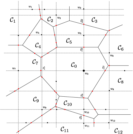
Figure 3. Ray-shooting and walking algorithms combined. Starting from chamber $\mathcal{C}_{0}$ we shoot and walk from chamber to chamber.

To obtain the multidegree, we only need one vertex. We computed the first vertex using Macaulay 2 [12] in a few days. Our ultimate goal was to compute the Newton polytope $\textrm{NP}(f)$, a much more difficult computational problem that took us many more months to complete. As a first attempt, we bound the number of lattice points in the polytope by the number of nonnegative lattice points of the given multidegree. Using the software LattE [3], we found that the number of monomials in 16 variables with multidegree $(110,55,55,55,55)$ is 5 529 528 561 944.

By construction, it is clear that the bottleneck of Algorithm 1 is in going through the list $\mathcal{F}$ of 6 865 824 cones. We can modify the algorithm to produce more than one vertex for each pass through the list. We do this in two ways. One is to process multiple objective vectors at once and save time by reducing the number of file readings and reusing the linear algebra computations for checking whether a cone meets a ray or not. Another way to produce more vertices is to keep track of the cones that we meet while ray-shooting, and use them to walk from chamber to chamber in the normal fan of $\textrm{NP}(f)$. This is described in Algorithm 2.

Input: A generic objective vector $w\in\mathbb{R}^{n}$, the vertex $\mathcal{P}^{w}$, and the set $\mathcal{S}:=\{(\sigma,i,t)\in\mathcal{F}\times\{1,2,\dots,n\}\times\mathbb{R}_{>0}~{}:~{}\sigma\cap(w-\mathbb{R}_{>0}e_{i})=\{w-te_{i}\}\}$. (This input is typically obtained from Algorithm 1.)

Output: The set of all vertices of $\mathcal{P}$ with objective vectors of the form $w-te_{i}$ for some $t\in\mathbb{R}_{>0}$ and $i\in\{1,2,\dots,n\}$.

for $i=1,2,\dots,n$ do  Let $\sigma_{1},\dots,\sigma_{m}$ be the cones that intersect the ray $w-\mathbb{R}_{>0}e_{i}$ transversely.

Let $t_{1},\dots,t_{m}\in\mathbb{R}_{>0}$ be such that $(\sigma_{k},i,t_{k})\in\mathcal{S}$ for $k=1,2,\dots,m$.

Order $\sigma_{1},\dots,\sigma_{m}$ so that t_1 = ⋯= t_k_1 ¡ t_k_1+1 = ⋯= t_k_2 ¡ ⋯¡ t_k_l+1 = ⋯= t_m:=t_k_l+1 . $v\leftarrow P^{w}$

for $j=1,2,\dots,l+1$ do  $\ell^{\sigma_{k_{j}}}\leftarrow$ primitive integral normal vector to $\sigma_{k_{j}}$ with $\ell^{\sigma_{k_{j}}}_{i}>0$;

$\displaystyle v\leftarrow v-\left(\sum_{k_{j-1}<k\leq k_{j}}m_{\sigma_{k}}\right)\cdot\ell^{\sigma_{k_{j}}}$, where $k_{0}=1$, $k_{l+1}=m$, and $m_{\sigma}$ denotes the multiplicity of $\sigma$.

Output $v$, and an objective vector in the line segment between $w-t_{k_{j}}e_{i}$ and $w-t_{k_{j+1}}e_{i}$, where $t_{k_{l+2}}:=\infty$.    

Algorithm 2 Walking: starting from an objective vector and corresponding vertex, compute the vertices obtained by changing the objective vector in negative coordinate directions.

Figure 4. Walking from vertex to vertex in $\textrm{NP}(f)\subset\mathbb{R}^{3}$. In dash lines, we plot the tropical variety. The picture represents the local structure around $v_{0}$.

On the polytope $\mathcal{P}$, this means walking from vertex $P^{w-te_{i}}$ to $P^{w-t^{\prime}e_{i}}$ for scalars $t^{\prime}>t>0$ corresponding to points between three consecutive intersection points, along an edge whose $i$-th coordinate is negative. If the vector $w$ is generic, then we can assume that $\sigma_{j}$ and $\sigma_{k}$ are parallel whenever they share an intersection point obtained by shooting from $w$ in a fixed coordinate direction. So we can use any of the cones in a parallel class to compute the edge direction of the wall we walk across. By adding up the multiplicities of the cones in each class, we get the lattice length of the edge of $\mathcal{P}$. This allows us to compute the coordinates of the vertices dual to the chambers we walk into. For each of these vertices found by walking from a known vertex, we also get an objective vector in the process. For example, any vector of the form $w-te_{i}$, where $t^{i}_{k_{j}}<t<t^{i}_{k_{j}+1}$, is an objective vector for the $j$-th vertex found in the walk in direction $-e_{i}$. We take $t^{i}_{m+1}$ as $\infty$. For numerical stability, we use exact arithmetic over the rational numbers. In particular, we always choose the new objective vectors to be integral.

Using a new vertex, with its associated objective vector, we can repeat the ray-shooting (Algorithm 1) and walking (Algorithm 2) again. The picture one should have in mind is that walking from chamber to chamber in the tropical side corresponds to walks from vertex to vertex in $\textrm{NP}(f)$ along edges normal to the codimension one cones traversed in the tropical hypersurface.

The combination of Algorithms 1 and 2 is illustrated in Figures 3 and 4. Starting from chamber $\mathcal{C}_{0}$ and an objective vector $w_{0}$, we shoot rays in minus the coordinate axes directions. The intersection points are indicated by their defining parameters $t^{i}_{j}$ (note that superscripts are omitted in the notation of Algorithm2). As we explain below, to speed up the computation of Algorithm 1 we first precompute the inverses of all suitable matrices of the form $M_{\sigma}:=(-e_{i}|r_{1}|\ldots|r_{15})$ where $\{r_{1},\ldots,r_{10}\}$ are generators of the cone $\sigma$ and $\{r_{11},\ldots,r_{15}\}$ span the lineality space in (3.5). Using this, the condition $(w_{0}-\lambda e_{i})\cap\sigma\neq\emptyset$ translates to the first eleven coordinates of the solution $X$ of $X^{t}=(M_{\sigma})^{-1}\cdot w_{0}$ being positive. Thus, we can easily use the same systems to test $(w_{0}+\lambda e_{i})\cap\sigma\neq\emptyset$, just changing the sign condition for the first coordinate of $X$. This small modification allows us to walk in sixteen new directions (the positive coordinate axes), and find new adjacent vertices to vertex $v_{0}$ starting form objective vector $w_{0}$. The step updating $v$ in Algorithm 2 should be $v\leftarrow v\bm{+}\left(\sum_{k_{j-1}<k\leq k_{j}}m_{\sigma_{k}}\right)\cdot\ell^{\sigma_{k_{j}}}$ instead of $v\leftarrow v-(\ldots)$ .

In Figure 3, the parameters $\lambda$ associated to the intersection points in these positive directions are denoted by $\tilde{t}^{i}_{j}$. The dashed arrows indicate the shooting directions. The points in the cones correspond to intersection points, whereas the points inside chambers are the objective vectors obtained for each vertice as described in Algorithm 2.

The dual walk in the Newton polytope is depicted in Figure 4. We start walking from vertex $v_{0}$ and via shooting we obtain the adjacent vertices $v_{5},v_{7},v_{8}$ and $v_{10}$. Notice that by this procedure we miss vertices $v_{4},v_{6}$ and $v_{9}$. However, we do get them if we start shooting from known adjacent chambers to $\mathcal{C}_{0}$. For example, $v_{6}$ can be computed if we shoot rays from chamber $\mathcal{C}_{8}$, followed by a shoot from chamber $\mathcal{C}_{6}$. Observe that this depends heavily on the choice of the objective vector $w_{6}$.

4.3. Implementation

A few notes about the implementation of our algorithms are in order. As we started working on the problem, we used Macaulay 2 [12] to do the ray-shooting (Algorithm 1). This script was fine for our first experiments, but it took three days to generate a single vertex of the polytope. It soon became evident that something faster was needed if we wanted to compute the entire polytope.

Our first step was to translate the Macaulay 2 script for Algorithm 1 into Python [17]. We chose that language because of its fast speed of development and availability of arbitrary precision integers, which were needed by our program. We always scale our objects (matrices and vectors) by positive integers so that our objects have integer coefficients. This step is crucial for numerical stability.

This new implementation brought the running time to about 10 hours. This was a remarkable improvement, but as the number of vertices of the polytope grew, we realized that something even faster was required. Therefore, we decided to resort to caching: instead of computing every inverse for each vector, we precomputed all the inverses and stored them using a binary format suitable for fast reading in Python (Pickles). This resulted in a file of a few tens of gigabytes, but dropped the time required for an individual ray-shooting procedure down to under three hours.

Once the Python prototype was working at a reasonable speed, we translated it into C++ [21], which brought the time required to do ray-shooting for a single vertex to 47 minutes on modest hardware. Moreover, ray-shooting for multiple objective vectors could be performed at the same time, thus amortizing the disk reads. Since we still needed large integers, we decided to use GMP [10] and its C++ interface.

The procedure for walking is a more or less straightforward translation of the pseudocode presented in Algorithm 2. It is still implemented in Python, because it takes a short amount of time to walk from a few hundred vertices at a time, and the simplicity of the script far outweights the time gains a C++ translation would provide.

4.4. Certifying facets

We now discuss how to certify certain inequalities as facets of a polytope $\mathcal{P}$ given by the dual tropical hypersurface $\mathcal{T}(f)$. By the duality between tropical hypersurfaces and Newton polytopes, each facet direction must be a ray in the tropical variety, equipped with the fan structure dual to $\mathcal{P}$. Lemma 4.4 provides a characterization for a vector in $\mathbb{R}^{n}$ to be a ray of $\mathcal{T}(f)$ with the inherited fan structure.

Lemma 4.4.

Let $w\in\mathbb{R}^{n}$ and $\mathcal{T}(f)$ be a tropical hypersurface given by a collection of cones, but with no prescribed fan structure. Let $d$ be the dimension of its lineality space. Let $\mathcal{H}=\{\sigma_{1},\ldots,\sigma_{l}\}$ be the list of cones containing $w$. Let $q_{i}$ be the normal vector to cone $\sigma_{i}$ for $i=1,\ldots,l$. Then, $w$ is a ray of $\mathcal{T}(f)$ if and only if $\{q_{1},\ldots,q_{l}\}$ generates a $(n-d-1)$-dimensional vector space if and only if $w$ is a facet direction of $\textrm{NP}(f)$.

Proof.

The vectors $\{q_{1},\dots,q_{l}\}$ are precisely the directions of edges in the face $\mathcal{P}^{w}$ of $\mathcal{P}:=\textrm{NP}(f)$. Since the lineality space of $\mathcal{T}(f)$ has dimension $d$, the polytope $\mathcal{P}$ has dimension $n-d$. The face $\mathcal{P}^{w}$ is a facet of $\mathcal{P}$ if and only if $q_{1},\dots,q_{l}$ span a $(n-d-1)$-dimensional vector space. ∎

For any objective vector $w\in\mathbb{R}^{n}$, we can compute a vertex in the face $\mathcal{P}^{w}$ by applying ray-shooting (Algorithm 1) to a generic objective vector $w^{\prime}$ in a chamber of the normal fan of $\mathcal{P}$ containing $w$. If we know that $w$ is in fact a facet direction of $\mathcal{P}$, then any vertex in $\mathcal{P}^{w}$ gives us the constant term $a$ in the facet inequality $w\cdot x\leq a$. This is used in Algorithm 3 for checking if a given inequality is a facet inequality of $\mathcal{P}$. This step will be essential to certify that our partial list of vertices is indeed the complete list of vertices of the polytope $\mathcal{P}$. We discuss this approach in Section 4.5.

Input: An inequality $w\cdot x\leq a$ and a tropical hypersurface (dual to polytope $\mathcal{P}$) given as a collection $\mathcal{F}$ of maximal cones.

Output: True if the inequality is a valid facet inequality of $\mathcal{P}$; False otherwise.

$\mathcal{N}\leftarrow\{\}$

for $\sigma\in\mathcal{F}$ do  if $w\in\sigma$ then  $\mathcal{N}\leftarrow\mathcal{N}\cup\{$normal vector to $\sigma\}$;     if $\dim\langle\mathcal{N}\rangle<n-d-1$ then  Output False   else  $w^{\prime}\leftarrow$ a vector in the interior of a chamber containing $w$

Compute the vertex $\mathcal{P}^{w^{\prime}}$ using ray-shooting (Algorithm 1).

if $w\cdot\mathcal{P}^{w^{\prime}}=a$ then  Output True   else  Output False    

Algorithm 3 Facet certificate: Check if a given inequality defines a facet of a polytope given by its normal fan.

We now explain how to obtain a vector in the interior of a chamber containing a facet direction $w$. We start by applying a modified version of Algorithm 1 with input vector $w$ and when we choose to shoot rays only in direction $-e_{1}$. Since $w$ is a ray of the tropical variety given by the collection $\mathcal{F}$, it belongs to some cones $\{\tau_{1},\ldots,\tau_{s}\}$ in $\mathcal{F}$. Let $\sigma_{1},\ldots,\sigma_{m}$ be the cones we intersect along the $-e_{1}$ direction (we allow intersections at boundary points of each cone). Note that we only pick those cones with $l_{1}^{\sigma_{j}}\neq 0$.

Now, we use Algorithm 2 with input vector $w$ and the set $\mathcal{S}$ corresponding to the cones $\sigma_{1},\ldots,\sigma_{m}$ and coordinate $1$. We assume $(\sigma_{k},1,t_{k})$ are ordered in increasing order, with all $t_{k}\geq 0$. We have two possible scenarios: either $\mathcal{S}$ is a subset of $\{0\}$ (that is, either the empty set or the set $\{0\}$) or it contains a positive real number. In the first case, we pick an objective vector $w_{1}=w-te_{1}$ for a positive number $t$ (for numerical stability, we choose $t$ to be a big rational number). In the second case, pick a number $t$ between zero and the first positive number $t_{j}$ from $\mathcal{S}$ and let $w_{1}=w-te_{1}$.

Third, we check if any cone in $\mathcal{F}$ contains $w_{1}$ or not. If not, then we let $w^{\prime}=w_{1}$. If yes, by the balancing condition, this means that there exists a maximal cone in the tropical variety containing both $w_{1}$ and $w$. Note that this cone may be obtained by gluing and/or subdividing some cones in $\mathcal{F}$. In this case then we proceed as above, replacing the original input vector $w$ by $w_{1}$ and shooting rays using coordinate $2$ instead of coordinate $1$. We repeat this process with all coordinates if necessary. Unless we have $w_{i}$ not contained in any cone of $\mathcal{F}$, at step $i$ we are guaranted to have a cone containing $w,w_{1},\ldots,w_{i-1},w_{i}$ by construction. By dimensionality argument, at most in sixteen steps, we obtain a vector $w_{i}$ not contained in any cone of $\mathcal{F}$. This vector will be the objective vector $w^{\prime}$ from Algorithm 3.

4.5. Completing the polytope

Once the ratio of new vertices computed with ray-shooting and walking decreases, the next natural question that arises is how to guarantee that we have found all vertices of our polytope. To answer this question, we construct the tangent cones at each vertex and try to certify their facets as facets of $\mathcal{P}$.

Definition 4.5.

Let $\mathcal{P}$ be a full-dimensional polytope in $\mathbb{R}^{N}$ and $v$ a vertex of $\mathcal{P}$. We define the tangent cone of $\mathcal{P}$ at $v$ to be the set:

$$\mathcal{T}^{\mathcal{P}}_{v}:=v+\mathbb{R}_{\geq 0}\langle w-v:w\in\mathcal{P}\rangle=v+\mathbb{R}_{\geq 0}\langle e:e\text{ edge of }\mathcal{P}\text{ adjacent to }v\rangle.$$

By construction, $\mathcal{T}^{\mathcal{P}}_{v}$ is a polyhedron with only one vertex and $\mathcal{P}\!\!=\!\!\bigcap_{v\text{ vertex of }\mathcal{P}}\mathcal{T}^{\mathcal{P}}_{v}\!\!$. In particular, an inequality defines a facet of $\mathcal{P}$ if and only if it defines a facet of one of the tangent cones.

Let $\mathcal{Q}$ be the convex hull of the vertices of $\mathcal{P}$ obtained via Algorithms 1 and 2. Our goal is to certify that $\mathcal{Q}=\mathcal{P}$. We proceed as follows. For each vertex $v$ of $\mathcal{Q}$ we wish to compare the tangent cones $\mathcal{T}_{v}^{\mathcal{Q}}$ and $\mathcal{T}_{v}^{\mathcal{P}}$. Since $\mathcal{Q}$ has over seventeen million vertices and $\mathcal{T}^{\mathcal{Q}}_{v}$ has no symmetry, straightforward convex hull computations are infeasible. If $\mathcal{T}^{\mathcal{Q}}_{v}=\mathcal{T}^{\mathcal{P}}_{v}$ then the extreme rays of $\mathcal{T}^{\mathcal{Q}}_{v}$ would be edge directions of $\mathcal{P}$, which we have already computed as the normal directions to the maximal cones of the tropical hypersurface, and which are 15 788 in total. For a fixed vertex $v\in\mathcal{Q}$ we compute all differences $w-v$ for all vertices $w$ of $\mathcal{Q}$ and test which of these vectors are parallel to edges of $\mathcal{P}$. The number of such edge directions in $\mathcal{T}^{\mathcal{Q}}_{v}$ is expected to be very small (usually under 30 in practice). Let $C_{v}^{\mathcal{Q},\mathcal{P}}$ be the convex hull of $v$ and all rays along the edge directions of $\mathcal{P}$ in $\mathcal{T}^{\mathcal{Q}}_{v}$. So we have $C_{v}^{\mathcal{Q},\mathcal{P}}\subseteq\mathcal{T}_{v}^{\mathcal{Q}}$ and we can test if $C_{v}^{\mathcal{Q},\mathcal{P}}\supseteq\mathcal{T}_{v}^{\mathcal{Q}}$ by computing facets of $C_{v}^{\mathcal{Q},\mathcal{P}}$ with Polymake [11]. If $C_{v}^{\mathcal{Q},\mathcal{P}}\supseteq\mathcal{T}_{v}^{\mathcal{Q}}$, we use Algorithm 3 to check whether each facet of $C_{v}^{\mathcal{Q},\mathcal{P}}$ is also a facet of $\mathcal{P}$. In this way, we can certify that $\mathcal{T}_{v}^{\mathcal{P}}\subseteq C_{v}^{\mathcal{Q},\mathcal{P}}$, hence $C_{v}^{\mathcal{Q},\mathcal{P}}=\mathcal{T}_{v}^{\mathcal{Q}}=\mathcal{T}_{v}^{\mathcal{P}}$. Certifying this for a vertex $v$ of $\mathcal{Q}$ in each symmetry class will give us $\mathcal{Q}=\bigcap_{v\textrm{ vertex of }Q}\mathcal{T}^{\mathcal{Q}}_{v}\supseteq\bigcap_{v\textrm{ vertex of }P}\mathcal{T}^{\mathcal{P}}_{v}=\mathcal{P}$, hence $\mathcal{Q}=\mathcal{P}$. We conclude:

Lemma 4.6.

Let $\mathcal{P}$ be a polytope and $\mathcal{Q}\subset\mathcal{P}$ be the convex hull of a subset of the vertices in $\mathcal{P}$. If all facets of $\mathcal{Q}$ are facets of $\mathcal{P}$, then $\mathcal{Q}\supset P$, so $\mathcal{Q}=\mathcal{P}$.

If we find that a facet $w\cdot x\leq a$ of $C_{v}^{\mathcal{Q},\mathcal{P}}$ is not a facet of $\mathcal{P}$ from Algorithm 3, then we are missing vertices adjacent to $v$ in $\mathcal{P}$ in this “false facet direction” $w$, so we can perturb $w$ so that it lies in a chamber of the normal fan of $\mathcal{P}$ and use ray-shooting (Algorithm 1) to find a new vertex in that direction. Using this method, we obtained the entire polytope in finite number steps. We describe the process of approximating $\mathcal{P}$ by a subpolytope $\mathcal{Q}$ in Algorithm 4. A schematic of complete tangent cones and incomplete tangent cones is depicted in Figure 5.

Input: A partial list $V$ of vertices of $\mathcal{P}$, a collection of cones $\mathcal{F}$ whose union is the tropical hypersurface, $d=$dimension of lineality space of the tropical hypersurface, and the group of symmetries of the tropical hypersurface.

Output: A complete list of vertices and facets of $\mathcal{P}$.

$\mathcal{S}\leftarrow\{\}$;

for representatives $v$ of orbits of $V$ do  $C^{\mathcal{Q},\mathcal{P}}_{v}\leftarrow$ convex hull of $v$ and all rays in directions $w-v$ where $w\in V$ and $w-v$ is normal to a cone in $\mathcal{F}$.

$A\leftarrow$ facets of $C^{\mathcal{Q},\mathcal{P}}_{v}$ (using Polymake).

for $z\in A$ do  if $z$ is a not facet of $\mathcal{P}$ by Algorithm 3 then  $w^{\prime}\leftarrow$ a vector in the interior of a chamber whose closure contains $z$.

Compute the vertex $\mathcal{P}^{w^{\prime}}$ using ray-shooting (Algorithm 1).

$V\leftarrow V\,\cup$ orbit of $\mathcal{P}^{w^{\prime}}$

Break and restart the outermost for-loop with the new $V$.   else  $\mathcal{S}\leftarrow\mathcal{S}\cup\{z\}$    

Output vertices $V$ and facets $\mathcal{S}$. 

Algorithm 4 Approximation of $\mathcal{P}$ by a subpolytope $\mathcal{Q}$: Given a partial list of vertices of a polytope $\mathcal{P}$ with no known complete list of vertices, we construct the subpolytope $\mathcal{Q}$ generated by this list. We certify when $\mathcal{Q}$ equals $\mathcal{P}$.

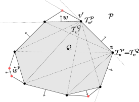
Figure 5. Approximation algorithm. We compute the tangent cones at vertices of $\mathcal{P}$ and we build a polytope $\mathcal{Q}\subset\mathcal{P}$. We certify if facets of $\mathcal{Q}$ are also facets of $\mathcal{P}$ by Algorithm 3. In the picture, we certify all facet directions in $\mathcal{T}^{\mathcal{Q}}_{v}$ containing vertex $v$ but we cannot certify the facet direction $w$ of the tangent cone $\mathcal{T}^{\mathcal{Q}}_{v^{\prime}}$. In addition, although we can certify the facet direction $w^{\prime}$ of $\mathcal{Q}$ as a true facet direction of $\mathcal{P}$, we will not be able to certify the constant corresponding to this facet direction of $\mathcal{P}$ since we are missing all its supporting vertices. The true constant will be obtained using Algorithm 3.

In the final stages of the computation, if we find that $C_{v}^{\mathcal{Q},\mathcal{P}}$ is a strict subcone of the tangent cone $\mathcal{T}^{\mathcal{Q}}_{v}$, we enumerated the rays $w-v$ (with $w\in V$) that lie in the difference $\mathcal{T}^{\mathcal{Q}}_{v}\backslash C_{v}^{\mathcal{Q},\mathcal{P}}$. If the number of such rays is small (no more than a few hundreds), we replace $C_{v}^{\mathcal{Q},\mathcal{P}}$ with the convex hull of $C_{v}^{\mathcal{Q},\mathcal{P}}$ and those rays (computed using Polymake) and proceed as in Algorithm 4. By executing Algorithm 4 in this way, we were able to compute and certify all vertices and facets of the polytope.

References

• [1] Tristram Bogart, Anders N. Jensen, David Speyer, Bernd Sturmfels, and Rekha R. Thomas. Computing tropical varieties. J. Symbolic Comput., 42(1-2):54–73, 2007.
• [2] María Angélica Cueto, Jason Morton, and Bernd Sturmfels. Geometry of the restricted Boltzmann machine. In M. Viana and H. Wynn, editors, Algebraic Methods in Statistics and Probability, Contemporary Mathematics. American Mathematical Society, 2010. To appear, E-print: arXiv:0908.4425.
• [3] Jesús A. De Loera, David Haws, Rraymond Hemmecke, Peter Huggins, Jeremy Tauzer, and Ruriko Yoshida. A user’s guide for latte v1.1. Available at http://www.math.ucdavis.edu/~latte, 2003.
• [4] Alicia Dickenstein. A world of binomials. Available at http://www.damtp.cam.ac.uk/user/na/FoCM/FoCM08/Talks/Dickenstein.pdf, 2008. Plenary lecture FoCM.
• [5] Alicia Dickenstein, Eva Maria Feichtner, and Bernd Sturmfels. Tropical discriminants. J. Amer. Math. Soc., 20(4):1111–1133 (electronic), 2007.
• [6] Mathias Drton, Bernd Sturmfels, and Seth Sullivant. Lectures on Algebraic Statistics, volume 39 of Oberwolfach Seminars. Birhkäuser, 2009.
• [7] Manfred Einsiedler, Mikhail Kapranov, and Douglas Lind. Non-Archimedean amoebas and tropical varieties. J. Reine Angew. Math., 601:139–157, 2006.
• [8] David Eisenbud. Commutative algebra with a view toward algebraic geometry, volume 150 of Graduate Texts in Mathematics. Springer-Verlag, New York, 1995.
• [9] Nicholas Eriksson, Kristian Ranestad, Bernd Sturmfels, and Seth Sullivant. Phylogenetic algebraic geometry. In Projective varieties with unexpected properties, pages 237–255. Walter de Gruyter GmbH & Co. KG, Berlin, 2005.
• [10] M. Galassi, J. Davies, J. Theiler, B. Gough, G. Jungman, P. Alken, M. Booth, and F. Rossi. GNU Scientific Library Reference Manual - Third Edition. Network Theory Ltd., 2009. http://www.gnu.org/software/gsl/.
• [11] Ewgenij Gawrilow and Michael Joswig. Polymake: a framework for analyzing convex polytopes. In Gil Kalai and Günter M. Ziegler, editors, Polytopes — Combinatorics and Computation, pages 43–74. Birkhäuser, 2000.
• [12] Daniel R. Grayson and Michael E. Stillman. Macaulay2, a software system for research in algebraic geometry. Available at http://www.math.uiuc.edu/Macaulay2/, 2009.
• [13] Anders N. Jensen. Gfan, a software system for Gröbner fans and tropical varieties. Available at http://www.math.tu-berlin.de/~jensen/software/gfan/gfan.html, 2009.
• [14] Joseph M. Landsberg and Laurent Manivel. On the ideals of secant varieties of Segre varieties. Found. Comput. Math., 4(4):397–422, 2004.
• [15] Joseph M. Landsberg and Jerzy Weyman. On the ideals and singularities of secant varieties of Segre varieties. Bull. Lond. Math. Soc., 39(4):685–697, 2007.
• [16] Nicolas Le Roux and Yoshua Bengio. Representational power of restricted Boltzmann machines and deep belief networks. Neural Comput., 20(6):1631–1649, 2008.
• [17] M. Lutz, D. Ascher, and F. Willison. Learning python. O’Reilly & Associates, Inc. Sebastopol, CA, USA, 1999.
• [18] Michael B. Monagan, Keith O. Geddes, K. Michael Heal, George Labahn, Stefan M. Vorkoetter, James McCarron, and Paul DeMarco. Maple 10 Programming Guide. Maplesoft, Waterloo ON, Canada, 2005.
• [19] Lior Pachter and Bernd Sturmfels. Algebraic Statistics for Computational Biology. Cambridge University Press, New York, NY, USA, 2005.
• [20] Jürgen Richter-Gebert, Bernd Sturmfels, and Thorsten Theobald. First steps in tropical geometry. In Idempotent mathematics and mathematical physics, volume 377 of Contemp. Math., pages 289–317. Amer. Math. Soc., Providence, RI, 2005.
• [21] B. Stroustrup et al. The C++ programming language. Addison-Wesley Reading, MA, 1997.
• [22] Bernd Sturmfels and Jenia Tevelev. Elimination theory for tropical varieties. Math. Res. Lett., 15(3):543–562, 2008.
• [23] Bernd Sturmfels, Jenia Tevelev, and Josephine Yu. The Newton polytope of the implicit equation. Mosc. Math. J., 7(2):327–346, 351, 2007.
• [24] Bernd Sturmfels and Josephine Yu. Tropical implicitization and mixed fiber polytopes. In Software for algebraic geometry, volume 148 of IMA Vol. Math. Appl., pages 111–131. Springer, New York, 2008.