Minimization of Ohmic losses for domain wall motion in a ferromagnetic nanowire

Abstract

We study current-induced domain-wall motion in a narrow ferromagnetic wire. We propose a way to move domain walls with a resonant time-dependent current which dramatically decreases the Ohmic losses in the wire and allows to drive the domain wall with higher speed without burning the wire. For any domain wall velocity we find the time-dependence of the current needed to minimize the Ohmic losses. Below a critical domain-wall velocity specified by the parameters of the wire the minimal Ohmic losses are achieved by dc current. Furthermore, we identify the wire parameters for which the losses reduction from its dc value is the most dramatic.

Introduction. In recent years there has been intense interest in applications of domain wall (DW) motion in ferromagnetic nanowires Par ; Allwood et al. (2005). This interest is mostly based on the possibility to store and exchange information by means of moving domain walls which separate the regions of magnetization parallel and anti-parallel to the wire. These regions with parallel and anti-parallel magnetization can be thought of as two bits, zero and one, of binary information storage.

DWs can be moved by a magnetic field Ono et al. (1999); Allwood et al. (2005) or electric current Yamaguchi et al. (2004); Par . For technological applications the current driving is preferred as magnetic field is difficult to apply locally to small wires. Thus, in this Letter we consider the current-driven DW devices. To achieve their highest performance it is important to minimize the losses on Joule heating in the wire, which are due to the resistance of the wire itself and the entire circuit. They are proportional to the time-averaged current square, $\langle J^{2}\rangle$. Their minimization has a twofold advantage. First, one can increase the maximum current which still does not destroy the wire by excessive heating and therefore move the DWs with a higher velocity, since the DW velocity increases with the applied current. Second, it creates the most energy efficient memory devices and also increases their reliability.

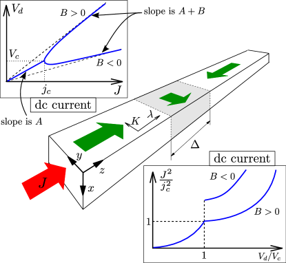
Figure 1: (color online) A sketch of a current driven domain wall in the ferromagnetic wire. The upper inset shows the dependence of drift velocity $V_{d}$ of DW on dc current $J$ for $B>0$ and $B<0$, see Eq. (2b). The slope at $J<j_{c}$ is given by $A$, while at $J\gg j_{c}$ it is $A+B$. The lower inset shows the power of Ohmic losses $p_{\rm{dc}}(V_{d}/V_{c})=J^{2}/j_{c}^{2}$ for dc current. For $B<0$ the power has a discontinuity at $V_{d}/V_{c}=1$.

To achieve these goals we propose to utilize a “resonant” time-dependent current, which allows to gain a significant reduction of Ohmic losses. We show that all thin wires can be characterized by three parameters obtained from dc-driven DW motion experiments: critical current $j_{c}$, drift velocity at the critical current $V_{c}$, and material dependent parameter $a>0$, which in particular depends on Gilbert damping $\alpha$ and non-adiabatic spin torque constant $\beta$. The parameter $a$ is just a ratio of the slopes of the drift velocity $V_{d}(J)$ at large and small dc-currents, see the upper inset of Fig. 1. Our main results are summarized in Fig. 2. We find the minimal power $\langle J^{2}\rangle$ needed to drive a DW with drift velocity $V_{d}$. Figures 2 (a) and (b) show the dependence of power $\langle J^{2}\rangle$ on $V_{d}$ for the optimal time-dependent current – red solid curves, and for dc current – black dashed curves, for two cases: (a) $a<1$ and (b) $a>1$. In Fig. 2 (a) the minimal power is given by dc current for $V_{d}<V_{c}$, but above $V_{c}$ there is a significant reduction in the heating power compared to dc current. Fig. 2 (b) shows that the power $\langle J^{2}\rangle$ is reduced in comparison with the dc case for $V_{d}>V_{c}v_{\rm{rc}}$. The (dimensionless) resonant critical velocity $v_{\rm{rc}}\leq 1$ and can be extracted from the dc-current measurements. For Permalloy using Moriya et al. (2008) we estimated $a\approx 0.5$, see Fig. 2 (a), where for $V_{d}\gtrsim V_{c}$ the power is less than $50\%$ of that for the dc current.

Figs. 2 (c) and (d) show the limiting cases of $a\ll 1$ (c) and $a\gg 1$ (d). We note that for small $\alpha$ and $\beta$, $a\approx\alpha/\beta$. If $a\ll 1$ ($\beta\gg\alpha$), Fig. 2 (c), for dc current the excessive heating power $\sim 1/a^{2}$ essentially limits the highest achievable drift velocity $V_{d}$ by $V_{c}$, whereas the resonant ac-current can move DWs with much higher $V_{d}$ (and still rather low power). In the opposite case $a\gg 1$, ($\beta\ll\alpha$), Fig. 2 (d), the power saving starts to be considerable at very small velocity $V_{d}$. If $\beta=0$ the dc-current power is finite even at $V_{d}\to 0$, while for the resonant ac-current the power linearly approaches zero at small $V_{d}$. Therefore, our approach gives a dramatic power reduction even in the least favorable cases $\beta\ll\alpha$ and $\beta\gg\alpha$, thus opening new doors for using materials with much wider range of $\beta$ for fast DW motion.

Model. DW in a ferromagnetic wire can be modeled by a Hamiltonian which contains exchange and dipolar interactions. In a thin wire, the latter can be approximated by two anisotropies: along the wire ($\lambda$) and transverse to it ($K$). A sketch of a wire with a DW of width $\Delta$ is shown in Fig. 1. The dynamics of magnetization $\mathbf{S}$ in a wire is described by Landau-Lifshitz-Gilbert (LLG) equation with the current $J$ Li and Zhang (2004); Thiaville et al. (2005),

$$\dot{\mathbf{S}}=\mathbf{S}\times\mathbf{H}_{e}-J\partial\mathbf{S}+\beta J\mathbf{S}\times\partial\mathbf{S}+\alpha\mathbf{S}\times\dot{\mathbf{S}},$$ (1)

where $\mathbf{H}_{e}=\delta\mathcal{H}/\delta\mathbf{S}$ is the effective magnetic field given by the Hamiltonian $\mathcal{H}$ of the system, $\alpha$ is Gilbert damping constant, $\beta$ is non-adiabatic spin torque constant, and $\partial=\partial/\partial z$. Furthermore, it can be shown Tretiakov and Ar. Abanov that in a thin wire the DW is a rigid spin texture for not too strong applied currents and its dynamics can be described in terms of only two collective coordinates (corresponding to the two softest modes of the DW motion), namely, the position of the DW along the wire $z_{0}$ and the rotation angle $\phi$ of the magnetization in the DW around the wire axis.

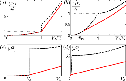
Figure 2: (color online) Minimal power of Ohmic losses $\overline{p}=\langle J^{2}\rangle/j^{2}_{c}$ as a function of drift velocity $V_{d}$ shown by solid line for (a) $a=0.5$ (b) $a=2$. The dashed line depicts $\overline{p}$ for dc current. A sketch of $\langle J^{2}\rangle(V_{d})$ shown by solid line in (c) for $\beta\gg\alpha$ ($a\ll 1$) and (d) for $\beta\ll\alpha$ ($a\gg 1$).

To describe the DW dynamics we need to find the equations of motion. For the two softest modes of the DW, $z_{0}(t)$ and $\phi(t)$, they can be found as an expansion in small current $J$ up to a linear in $J$ order. Due to the translational invariance $\dot{z}_{0}$ and $\dot{\phi}$ cannot depend on $z_{0}$. In addition, to the first order in small transverse anisotropy $K$, $\dot{\phi}$ and $\dot{z}_{0}$ are proportional to the first harmonic $\sin(2\phi)$. Then the most general equations of DW motion are

$$\dot{\phi}=C[J-j_{c}\sin(2\phi)],$$ (2a)

$$\dot{z}_{0}=AJ+B[J-j_{c}\sin(2\phi)],$$ (2b)

where $J(t)$ is, in general, a time-dependent current whose frequency is not too high to create spin waves and other excitations in the wire. Coefficients $A$, $B$, $C$, and critical current $j_{c}$ can be calculated for a particular model in terms of $\alpha$, $\beta$ and other microscopic parameters by means of deriving Eqs. (2) from LLG equation (1). However, we emphasize that Eqs. (2), with coefficients $A$, $B$, $C$, and $j_{c}$ determined directly from dc-current experiment for each particular wire, have more general validity than just being derived from LLG, e.g., due to the complicated influence of disorder and internal DW dynamics Min et al. (2010). Namely, the value of $j_{c}$ is defined as the endpoint of the linear regime of the time-averaged (drift) velocity $V_{d}=\langle\dot{z}_{0}(J)\rangle$, see the upper inset of Fig. 1. The linear slope of $V_{d}(J)$ below $j_{c}$ determines constant $A$. The slope of $V_{d}(J)$ at large $J$ gives $A+B$. Constant $C$ one can obtain, e.g., from the measurements of the DW electromotive force Yang et al. (2009); Liu for dc current.

DC current. For the dc current applied to the wire the DW dynamics governed by Eqs. (2) can be obtained explicitly Tretiakov and Ar. Abanov . For $J<j_{c}$ and $A\neq 0$ the DW moves along the wire but does not rotate around its axis. It only tilts on angle $\phi_{0}$ from the transverse-anisotropy easy axis ($y$ axis) given by condition $\sin(2\phi_{0})=J/j_{c}$. The drift velocity is given by $V_{d}=AJ$, see Eq. (2b). At $J=j_{c}$ the magnetization angle becomes perpendicular to the easy axis, $\phi_{0}=\pi/2$. For $J>j_{c}$ the DW both moves and rotates, and Eqs. (2) give $V_{d}=AJ+B\sqrt{J^{2}-j_{c}^{2}}$ Tretiakov and Ar. Abanov .

The influence of the spin structure on the current is negligible. The largest losses in the system are the Ohmic losses of the current. The power of Ohmic losses is proportional to $J^{2}$. Therefore, at $J<j_{c}$ the current is $J=V_{d}/A$ and the power of Ohmic losses is $\mathcal{P}_{\rm{dc}}=J^{2}=V_{d}^{2}/A^{2}$. It is instructive to introduce the dimensionless variables for time, drift velocity, current, and power. Using $V_{c}=Aj_{c}\simeq K\Delta$ we find 

$$\tau=Cj_{c}t,\quad v_{d}=V_{d}/V_{c},\quad j=J/j_{c},\quad p=\mathcal{P}/j_{c}^{2}.$$ (3)

Using Eq. (3) we find $p_{\rm{dc}}=v_{d}^{2}$ for $v_{d}<1$.

For currents above $j_{c}$ the dimensionless power $p_{\rm{dc}}$ is given in terms of dimensionless drift velocity $v_{d}=j+(B/A)\sqrt{j^{2}-1}$ as $p_{\rm{dc}}(v_{d})=j^{2}$, see the lower inset of Fig. 1. Thus, it is quadratic in $v_{d}$, and at $v_{d}\gg 1$ it approaches $p_{\rm{dc}}=A^{2}v_{d}^{2}/(B+A)^{2}+B/(B+A)$. For $B>0$ right above $v_{d}=1$, it is approximated by $p_{\rm{dc}}=1+(A/B)^{2}(v_{d}-1)^{2}$. For $B<0$ the power has a discontinuity at $v_{d}=1$.

Minimization of Ohmic losses by time-dependent current. In this part we minimize the Ohmic losses while keeping the DW moving with a given drift (average) velocity. Equations of motion (2) are correct even when the current depends on time. In general, the DW motion has some period $T$ and current $j(\tau)$ must be a periodic function with the same $T$ to minimize the Ohmic losses.

In the following it is more convenient to measure the angle from the hard axis instead of easy axis and to scale it by factor of 2, so that $2\phi=\theta-\pi/2$. Also, we introduce the ratio of slopes of $V_{d}(J)$ at large and small currents $a=(A+B)/A$. Then using Eq. (2a) the dimensionless current becomes

$$j(\tau)=\dot{\theta}/2-\cos\theta,$$ (4)

where $\dot{\theta}=\partial\theta/\partial\tau$. Averaging Eq. (2b) over dimensionless period $T$ we find

$$v_{d}=\frac{a}{2}\langle\dot{\theta}\rangle-\langle\cos\theta\rangle,$$ (5)

where $\langle\dots\rangle=\frac{1}{T}\int_{0}^{T}\dots d\tau$ is the time averaging.

To minimize the power of Ohmic losses $\overline{p}$ averaged over time we need to find the minimum of $\langle j^{2}(\tau)\rangle$ at fixed $v_{d}$ given by Eq. (5),

$$\overline{p}=\left\langle\left(\frac{\dot{\theta}}{2}-\cos\theta\right)^{2}-2\rho\left(\frac{a}{2}\dot{\theta}-\cos\theta-v_{d}\right)\right\rangle.$$ (6)

Here to account for the constraint given by Eq. (5) we used a Lagrange multiplier $2\rho$, with $\rho$ being an arbitrary dimensionless constant. Note that the cross term $\sim\int\dot{\theta}\cos\theta\,d\tau^{\prime}$ and the term $\sim\int\dot{\theta}\,d\tau^{\prime}$ can be dropped for the minimization procedure as they are full derivatives.

Power (6) can be considered as an effective action for a hypothetical particle of mass $1/2$ in a periodic potential field, and its minimization leads to the equation of motion

$$\frac{\ddot{\theta}}{2}=-\frac{\partial U}{\partial\theta},\qquad U(\theta,\rho)=-\cos^{2}\theta-2\rho\cos\theta.$$ (7)

It can be reduced to the first order differential equation

$$\dot{\theta}=\pm 2\sqrt{d-U(\theta,\rho)},$$ (8)

where $d$ is an arbitrary integration constant. Note that changing $\rho\to-\rho$ in $U$ of Eq. (7) is equivalent to changing $\theta\to\pi+\theta$, so below we consider only positive $\rho$. The potential has a minimum at $\theta=0$ with $U_{\rm{min}}=2\rho-1$ for any $\rho\geq 0$. For $\rho<1$ it has also minimum at $\theta=\pm\pi$ with $U(\pm\pi)=-2\rho-1$ and the maximum at $\cos\theta_{\rho}=-\rho$ with $U(\pm\theta_{\rho})=\rho^{2}$. For $\rho>1$ it has maximum at $\theta=\pm\pi$ with $U(\pm\pi)=2\rho-1$.

According to Eq. (8) there are two different regimes: i) the rocking regime where $d<\rm{max}[U(\theta,\rho)]$ in which case $\theta$ is bounded, and the particle oscillates in potential well $U(\theta)$, see Fig. 3; and ii) the rotational regime where $d>\rm{max}[U(\theta,\rho)]$ in which case the magnetization in the DW rotates. Below we consider these regimes separately.

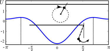
Figure 3: (color online) Potential $U(\theta)$ in which a “particle” is moving in the rocking (pendulum-like) and rotational regimes.

Rocking regime. In this regime the motion of $\theta$ mimics pendulum motion. The particle rocks between the two turning points $-\theta_{0}$ and $\theta_{0}$ given by the condition $d=U(\pm\theta_{0},\rho)$. At these points $\dot{\theta}=0$. Since $\theta$ is a bounded function $\langle\dot{\theta}\rangle=0$ and the averaged velocity becomes $v_{d}=-\langle\cos\theta\rangle$. The averaging is done over a period of one complete oscillation,

$$T=\int_{-\theta_{0}}^{\theta_{0}}\frac{d\theta}{\sqrt{d-U(\theta,\rho)}},$$ (9)

and according to Eq. (6) the power is given by

$$\overline{p}=\langle{\dot{\theta}}^{2}\rangle/4+\langle\cos^{2}\theta\rangle.$$ (10)

Most generally $\theta$ depends on time. For any $\theta(\tau)$, however, $\langle\cos^{2}\theta\rangle\geq\langle\cos\theta\rangle^{2}$. Then from Eq. (10) follows $\overline{p}\geq\langle\dot{\theta}^{2}\rangle/4+\langle\cos\theta\rangle^{2}=\langle\dot{\theta}^{2}\rangle/4+v_{d}^{2}\geq v_{d}^{2}=p_{\rm{dc}}$. Thus, in the bounded regime the power of Ohmic losses is minimal for dc current and is given by $\overline{p}=v_{d}^{2}$.

Rotational regime. Next we study the case when $d>\rm{max}[U(\theta,\rho)]$, so that angle $\theta$ is unbounded. It corresponds to the rotational motion of the transverse to the wire component of the DW magnetization. Note that in the rotational regime the term in Eq. (5) with $\langle\dot{\theta}\rangle$ should be kept because $\theta$ is not bounded. The time it takes for $\theta$ to make a full rotation from $-\pi$ to $\pi$ defines the period $T$. Then the period, drift velocity, and power, according to Eq. (10), are given by

$$T = \frac{1}{2}\int_{-\pi}^{\pi}\frac{d\theta}{\sqrt{d-U(\theta,\rho)}},$$ (11a)

$$v_{d} = \frac{\pi a}{T}-\frac{1}{2T}\int_{-\pi}^{\pi}\!\!\frac{\cos\theta\,d\theta}{\sqrt{d-U(\theta,\rho)}},$$ (11b)

$$\overline{p} = \frac{1}{2T}\int_{-\pi}^{\pi}\!\!\frac{d-U(\theta,\rho)+\cos^{2}\theta}{\sqrt{d-U(\theta,\rho)}}d\theta.$$ (11c)

This system of equations, after minimizing the power $\overline{p}$ with respect to both $d$ and $\rho$ at fixed $v_{d}$, gives $\overline{p}(v_{d})$. One can either directly perform a numerical minimization of Eq. (11) or alternatively try to find the minimization condition for $\overline{p}$ analytically. We have followed both routes.

The minimization of Eqs. (11) infers that $\partial\overline{p}/\partial\rho|_{v_{d}}=0$ from which one can find Ohm

$$\int_{-\pi}^{\pi}\!\sqrt{d-U(\theta,\rho)}d\theta=2\pi a\rho.$$ (12)

This equation gives the relationship between $d$ and $\rho$. Solving it together with Eq. (11b) one finds $d$ and $\rho$ in terms of $v_{d}$. They are then substituted into $\overline{p}=2\rho v_{d}-d$ which follows from Eqs. (11c) and (12). The motion is unbounded when $d>\rm{max}[U(\theta,\rho)]$, see Eq. (8), which leads to $d>\rho^{2}$ for $\rho<1$ and $d>2\rho-1$ for $\rho>1$.

The results for the minimal power of Ohmic losses $\overline{p}(v_{d})$ are presented in Fig. 2. For $a<1$, see e.g. Fig. 2 (a), at $v_{d}<v_{\rm{rc}}=1$ the minimal power $\overline{p}$ coincides with the one given by dc current, whereas at $v_{d}>1$ it is significantly lower than $p_{\rm{dc}}$. Immediately above $v_{d}=1$ we find that there is a range of $v_{d}$ where $\overline{p}=1+2\rho_{0}(v_{d}-1)$ with $\rho_{0}(a)>1$ given by Eq. (12) with $d=2\rho-1$. Therefore, $\overline{p}$ is linear in $v_{d}$ right above $v_{\rm{rc}}=1$.

For $a>1$, see e.g. Fig. 2 (b), we show Ohm that there is a critical velocity $v_{\rm{rc}}<1$, such that at $v_{d}<v_{\rm{rc}}$ the power of Ohmic losses is $\overline{p}=v_{d}^{2}=p_{\rm{dc}}$. Above $v_{\rm{rc}}$ one can minimize the Ohmic losses by moving DW with resonant current pulses. Right above $v_{\rm{rc}}$ there is a certain range of $v_{d}$ where $d\simeq\rho^{2}$, and therefore we find $\overline{p}=2\rho_{0}v_{d}-\rho_{0}^{2}$ with $\rho_{0}(a)<1$ given by Eq. (12) with $d=\rho^{2}$. The critical velocity is found as $v_{\rm{rc}}=\rho_{0}(a)$. For $a\gg 1$ (corresponding to non-adiabatic spin transfer torque coefficient $\beta\ll\alpha$, c.f. Eq. (1)) we find $v_{\rm{rc}}\simeq 2/(\pi a)$ and therefore for $v_{d}\gg v_{\rm{rc}}$ we obtain $\overline{p}=4v_{d}/(\pi a)$.

We show that at large $v_{d}$ the minimal power is always smaller than $p_{\rm{dc}}$. Note that for $d\gg 1$ Eq. (12) gives $d=a^{2}\rho^{2}$. Using it we find that the difference between them approaches $p_{\rm{dc}}-\overline{p}=(1-1/a)^{2}/2$ at $v_{d}\gg 1$.

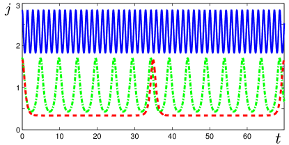
Figure 4: (color online) Current $j$ as a function of time $\tau$ at velocities $v_{d}=0.5$ (dashed line), $v_{d}=1.5$ (dot-dashed line), and $v_{d}=4.5$ (solid line) in the rotational regime for $a=2$.

Optimal current. For $v_{d}<v_{\rm{rc}}$ the optimal current coincides with the dc current. Above $v_{\rm{rc}}$ the resonant current $j(t)$ is plotted in Fig. 4 for different velocities $v_{d}$ in the case $a=2$. At small $v_{d}$ the current is given by $j(\tau)=-2\cos(\theta(\tau))-v_{\rm{rc}}$ for $\cos(\theta(\tau))<-v_{\rm{rc}}$ and by $j(\tau)=v_{\rm{rc}}$ for $\cos(\theta(\tau))>-v_{\rm{rc}}$. At $v_{d}\gg 1$ the current is approximated by $j\approx v_{d}/a+[(1-a)/a]\cos\theta$.

In general, at $v_{d}>v_{\rm{rc}}$ the current’s maximum $j_{\rm{max}}$ increases from $2-v_{\rm{rc}}$ at small enough $v_{d}\lesssim 1$ up to $j_{\rm{max}}\approx v_{d}/a$ at $v_{d}\gg 1$. The current’s minimum increases monotonically from small positive values $j_{\rm{min}}=v_{\rm{rc}}$ at $v_{d}\sim 1$ up to $j_{\rm{min}}=j_{\rm{max}}-2|1-a|/a$ at $v_{d}\gg 1$. At $v_{d}\lesssim 1$ (for $a>1$) the time between the current picks decreases with increasing velocity as $T\simeq(\pi a-2\arcsin v_{\rm{rc}})/(v_{d}-v_{\rm{rc}})$, whereas the pick’s width is given by $\approx 1.3/\sqrt{(1-v_{\rm{rc}})}$, which is independent of $v_{d}$. Therefore, at small $v_{d}-v_{\rm{rc}}$ the picks are widely separated, then as $v_{d}$ increases the time between the picks decreases. At $v_{d}\gg 1$ the optimal current has a large constant component, which is close to but smaller than the dc current for the same $v_{d}$, and has small-amplitude ac modulations with a period $T\approx\pi a/v_{d}$ on top of it.

Summary. We have studied the current driven DW dynamics in thin ferromagnetic wires. We have found the ultimate lower bound for the Ohmic losses in the wire for any DW drift velocity $V_{d}$. The explicit time-dependence of current, see Fig. 4, has been found which minimizes the Ohmic losses. We have shown that the use of these specific current pulses instead of applying dc current can help to significantly reduce heating of the wire for any $V_{d}$. Even in the limiting cases of the systems with weak ($\beta\ll\alpha$) or strong ($\beta\gg\alpha$) non-adiabatic spin transfer torque, where the power of Ohmic losses is high for dc currents, the optimized ac current gives significant reduction in heating power thus greatly expanding the range of materials which can be used for spintronic devices Allwood et al. (2005); Par .

We are grateful to J. Sinova for valuable discussions. This work was supported by the NSF Grant No. 0757992 and Welch Foundation (A-1678).

Supplementary material for “Minimization of Ohmic losses for domain wall motion in a ferromagnetic nanowire”

I Minimization procedure

As described in the main part of the Letter we study a domain-wall dynamics under the influence of a time-dependent current. The equations of motion for the domain wall in the thin ferromagnetic wire take the form of Eqs. (2) of the main part of this Letter. To obtain the results of the main part, we use the dimensionless variables introduced in Eq. (3) of the main part.

In order to minimize the power of Ohmic losses we need to find a minimum of the average $j^{2}$,

$$\overline{p}=\langle j^{2}(\tau)\rangle$$ (13)

at a fixed drift velocity $v_{d}$. From Eqs. (2) of the main part of the Letter we find

$$j(\tau)=\frac{1}{2}\dot{\theta}-\cos\theta,$$ (14)

$$v(\tau)=\frac{a}{2}\dot{\theta}-\cos\theta,$$ (15)

$$v_{d}=\frac{a}{2}\langle\dot{\theta}\rangle-\langle\cos\theta\rangle,$$ (16)

$$\overline{p}=\left\langle\left(\frac{1}{2}\dot{\theta}-\cos\theta\right)^{2}\right\rangle,$$ (17)

where $\dot{\theta}=\partial\theta/\partial\tau$ and the averaging is performed over the dimensionless period $T$ of the magnetization oscillations. To find the minimum of power at fixed drift velocity we introduce a Lagrange multiplier $2\rho$ and minimize the functional

$$\overline{p}=\left\langle\left(\frac{1}{2}\dot{\theta}-\cos\theta\right)^{2}\right\rangle-2\rho\left(\frac{a}{2}\langle\dot{\theta}\rangle-\langle\cos\theta\rangle-v_{d}\right),$$ (18)

where $\langle\dots\rangle=T^{-1}\int_{0}^{T}\dots d\tau$ is the averaging over time. Then it follows

$$\overline{p}=\frac{1}{T}\int_{0}^{T}\left(\frac{1}{4}\dot{\theta}^{2}+\cos^{2}\theta+2\rho\cos\theta\right)d\tau,$$ (19)

where we dropped all the terms which are full derivatives and therefore do not give any contribution to the minimized power.

The minimization of Eq. (19) gives the following equation of motion

$$\frac{1}{2}\ddot{\theta}=-\partial_{\theta}U(\theta,\rho),$$ (20)

$$U(\theta,\rho)=-\cos^{2}\theta-2\rho\cos\theta.$$ (21)

Its solution is given by

$$\dot{\theta}=\pm 2\sqrt{d-U(\theta,\rho)}$$ (22)

where $d$ is an arbitrary constant of integration. We note, that changing $\rho\rightarrow-\rho$ is equivalent to changing $\theta\rightarrow\pi+\theta$, so we only need to consider positive $\rho$. The extrema of potential $U$ are

$$\begin{array}[]{lll}\theta=0,&U(0,\rho)=-1-2\rho,\\ \theta=\pm\pi,&U(\pm\pi,\rho)=-1+2\rho,\\ \cos\theta_{\rho}=-\rho,&U(\pm\theta_{\rho},\rho)=\rho^{2},\end{array}$$ (23)

where the last extremum exists only for $\rho<1$.

We see that there are two different cases: i) rocking – when $d$ is smaller then the maximum of $U(\theta,\rho)$, and ii) rotating – when $d$ is larger then the maximum of $U(\theta,\rho)$. We consider them separately.

II Rocking regime

In this case there is an angle $\theta_{0}$ such that $d=U(\theta_{0},\rho)$. Then we have the oscillating motion between $-\theta_{0}$ and $\theta_{0}$ and back. The period of one complete oscillation, as well as the drift velocity and power are given by

$$T = \int_{-\theta_{0}}^{\theta_{0}}\frac{d\theta}{\sqrt{U(\theta_{0},\rho)-U(\theta,\rho)}},$$ (24)

$$v_{d} = -\langle\cos\theta\rangle=-\frac{1}{T}\int_{-\theta_{0}}^{\theta_{0}}\frac{\cos\theta\,d\theta}{\sqrt{U(\theta_{0},\rho)-U(\theta,\rho)}},$$ (25)

$$\overline{p} = \left\langle\frac{1}{4}\dot{\theta}^{2}+\cos^{2}\theta\right\rangle$$ (26)

$$= \frac{1}{T}\int_{-\theta_{0}}^{\theta_{0}}\frac{U(\theta_{0},\rho)-U(\theta,\rho)+\cos^{2}\theta}{\sqrt{U(\theta_{0},\rho)-U(\theta,\rho)}}d\theta.$$

II.1 dc current

In the case of dc current $\theta=\mbox{const}$ equation (22) gives $\theta=\theta_{0}$, then (20) requires that $\theta_{0}$ is an extremum of $U(\theta,\rho)$, there are three possibilities $\theta=\{0,\pi,\theta_{\rho}\}$, for them we get $v_{d}=\{-1,1,\rho\}=j$, and $p=\{1,1,\rho^{2}\}$. So we see, that $p=v_{d}^{2}$.

II.2 ac current

Now we take $\theta$ changing with time. From the condition

$$\left\langle\left(\langle\cos\theta\rangle-\cos\theta\right)^{2}\right\rangle\geq 0,$$ (27)

it follows that

$$\langle\cos^{2}\theta\rangle\geq\langle\cos\theta\rangle^{2}.$$ (28)

Then the power $\overline{p}$ satisfies the condition

$$\overline{p} = \frac{1}{4}\left\langle\dot{\theta}^{2}\right\rangle+\left\langle\cos^{2}\theta\right\rangle\geq\frac{1}{4}\left\langle\dot{\theta}^{2}\right\rangle+\left\langle\cos\theta\right\rangle^{2}$$ (29)

$$= \frac{1}{4}\left\langle\dot{\theta}^{2}\right\rangle+v_{d}^{2}\geq v_{d}^{2}$$

Thus, we see that in the rocking regime the dc current minimizes the Ohmic losses.

III Rotating regime

In this section we study the rotational regime. In this case $\theta$ makes a full rotation from $-\pi$ to $\pi$. The period of one complete rotation, as well as the drift velocity and power are given by Eqs. (11) in the main part of this Letter, i.e.

$$T\! =\! \frac{1}{2}\int_{-\pi}^{\pi}\frac{d\theta}{\sqrt{d-U(\theta,\rho)}},$$ (30)

$$v_{d}\! =\! \frac{a}{2}\langle\dot{\theta}\rangle-\langle\cos\theta\rangle=\frac{\pi a}{T}-\frac{1}{2T}\int_{-\pi}^{\pi}\!\frac{\cos\theta\,d\theta}{\sqrt{d-U(\theta,\rho)}},$$ (31)

$$\overline{p}\! =\! \left\langle\frac{1}{4}\dot{\theta}^{2}+\cos^{2}\theta\right\rangle=\frac{1}{2T}\int_{-\pi}^{\pi}\frac{d-U(\theta,\rho)+\cos^{2}\theta}{\sqrt{d-U(\theta,\rho)}}d\theta,$$

where $a=(A+B)/A$.

III.1 dc current

In this case $j=\mbox{const}$ and according to Eq. (14) we find

$$\frac{1}{2}\dot{\theta}-\cos\theta=j,\quad T=\int_{0}^{2\pi}\!\frac{d\theta}{j+\cos\theta}=\frac{\pi}{\sqrt{j^{2}-1}},$$

$$\langle\cos\theta\rangle=-j+\frac{1}{2}\langle\dot{\theta}\rangle,\quad v_{d}=\frac{a-1}{2}\langle\dot{\theta}\rangle+j.$$ (33)

Since $\langle\dot{\theta}\rangle=2\pi/T$ we obtain

$$v_{d}=\frac{a-1}{2}\sqrt{j^{2}-1}+j,\quad p_{\rm{dc}}=j^{2},\quad j>1.$$ (34)

In particular for $j\gg 1$ we find

$$p_{\rm{dc}}\approx\frac{4}{(1+a)^{2}}v_{d}^{2}+\frac{a-1}{a+1}.$$ (35)

III.2 ac current

The same trick as in Sec. II.2 gives

$$\overline{p}\geq\frac{v_{d}^{2}}{1+a^{2}}+\left(\frac{\sqrt{1+a^{2}}}{2}\langle\dot{\theta}\rangle-\frac{a}{\sqrt{1+a^{2}}}v_{d}\right)^{2},$$

and we can only conclude that the power is no smaller than quadratic in $v_{d}$.

III.2.1 Derivation of minimization condition, Eq. (12)

In this section we derive the minimization condition, Eq. (12) of the main part of the Letter. We rewrite Eqs. (11) of the main part in the following way

$$T=\frac{1}{2}\int_{-\pi}^{\pi}\frac{d\theta}{\sqrt{d-U(\theta,\rho)}}$$ (36)

$$Tv_{d}=\pi a-\frac{1}{2}\int_{-\pi}^{\pi}\frac{\cos\theta\,d\theta}{\sqrt{d-U(\theta,\rho)}},$$ (37)

$$\overline{p}=2\rho v_{d}-d+\frac{1}{T}\int_{-\pi}^{\pi}\left[\sqrt{d-U(\theta,\rho)}-a\rho\right]\!d\theta.$$ (38)

The minimization of $\overline{p}$ means that $\partial\overline{p}/\partial\rho|_{v_{d}}=0$, and we find

$$\left.\frac{\partial\overline{p}}{\partial\rho}\right|_{v_{d}}=-\left.\frac{\partial T}{\partial\rho}\right|_{v_{d}}\frac{1}{T^{2}}\int_{-\pi}^{\pi}\left[\sqrt{d-U(\theta,\rho)}-a\rho\right]d\theta=0$$ (39)

There are two possibilities to satisfy this condition

$$\left.\frac{\partial T}{\partial\rho}\right|_{v_{d}}=0,\quad\mbox{or}$$ (40)

$$\int_{-\pi}^{\pi}\left[\sqrt{d-U(\theta,\rho)}-a\rho\right]d\theta=0.$$ (41)

Note that there is also a possibility $T=\infty$ but it corresponds to a dc-current case.

First we consider the possibility given by Eq. (40). Differentiating Eqs. (36) and (37) with respect to $\rho$ at fixed $v_{d}$ and using Eq. (40), we obtain

$$0\!\! =\!\! \left.\frac{\partial d}{\partial\rho}\right|_{v_{d}}\int_{-\pi}^{\pi}\frac{d\theta}{[d-U(\theta,\rho)]^{3/2}}+2\!\int_{-\pi}^{\pi}\frac{\cos\theta\,d\theta}{[d-U(\theta,\rho)]^{3/2}}$$

$$0\!\! =\!\! \left.\frac{\partial d}{\partial\rho}\right|_{v_{d}}\int_{-\pi}^{\pi}\frac{\cos\theta\,d\theta}{[d-U(\theta,\rho)]^{3/2}}+2\!\int_{-\pi}^{\pi}\frac{\cos^{2}\theta\,d\theta}{[d-U(\theta,\rho)]^{3/2}}$$

Combining these two equations, we find

$$\left[\int_{-\pi}^{\pi}\frac{\cos\theta\,d\theta}{[d-U(\theta,\rho)]^{3/2}}\right]^{2}=\int_{-\pi}^{\pi}\frac{d\theta}{[d-U(\theta,\rho)]^{3/2}}\int_{-\pi}^{\pi}\frac{\cos^{2}\theta^{\prime}\,d\theta^{\prime}}{[d-U(\theta^{\prime},\rho)]^{3/2}}$$ (42)

Note that this is a standard Bunyakovsky (Cauchy – Schwarz) inequality and it never becomes an equality except for $\theta=0$. Therefore, we conclude that in the rotational regime the minimization condition is given by Eq. (41). Then, the system of equations which we need to solve is

$$\int_{-\pi}^{\pi}\left[\sqrt{d-U(\theta,\rho)}-a\rho\right]d\theta=0,$$ (43)

$$v_{d}T=\pi a-\frac{1}{2}\int_{-\pi}^{\pi}\frac{\cos\theta\,d\theta}{\sqrt{d-U(\theta,\rho)}},$$ (44)

$$\overline{p}=2\rho v_{d}-d,$$ (45)

where the second equation is just Eq. (37) with $T$ given by Eq. (36). Eq. (43) provides the correspondence between parameters $\rho$ and $d$. Solving together the system of equations (43) and (44) yields $\rho(v_{d})$ and $d(v_{d})$. They are then substituted into Eq. (45) to find $\overline{p}(v_{d})$. In general, the system of equations (43) and (44) has to be solved numerically. However, in the limiting cases of small and large drift velocities $v_{d}$ the result for $\overline{p}(v_{d})$ can be obtained analytically. Below we solve these limiting cases.

III.3 Large $v_{d}$

First we consider the case of large $v_{d}$ which corresponds to large parameters $d$. At $d\gg 1$ Eq. (43) gives $d=a^{2}\rho^{2}$. Using it we find that the difference $p_{\rm{dc}}-\overline{p}=(a-1)^{2}/2a^{2}$ at $v_{d}\gg 1$. Thus, at large $v_{d}$ the minimal power is always smaller than $p_{\rm{dc}}$.

III.4 Small $v_{d}$

We recall that in the rotational regime the motion is unbounded and therefore $d>\rm{max}[U(\theta,\rho)]$, see Eq. (22). This leads to $d>\rho^{2}$ for $\rho<1$ and $d>2\rho-1$ for $\rho>1$. We show that it is possible to find analytical results for $\overline{p}(v_{d})$ when $d=\rho^{2}+\epsilon$ or $d=2\rho-1+\epsilon$ and $\epsilon\ll 1$. Below we consider these two cases separately.

III.4.1 $0<d<1$

For the case $d=\rho^{2}+\epsilon$ with $\epsilon\ll 1$, we find

$$T(\epsilon,\rho) = \frac{1}{2}\int_{-\pi}^{\pi}\frac{d\theta}{\sqrt{\epsilon+(\rho+\cos\theta)^{2}}}$$ (46)

$$T(\epsilon,\rho)v_{d} = \pi a-\frac{1}{2}\int_{-\pi}^{\pi}\frac{\cos\theta\,d\theta}{\sqrt{\epsilon+(\rho+\cos\theta)^{2}}}$$ (47)

In particular if $\rho=0$, one can find that $T=\ln(16/\epsilon)$, $v_{d}=\pi a/\ln(16/\epsilon)$, and $\overline{p}=4/\ln(16/\epsilon)=4v_{d}/(\pi a)$.

From Eqs. (46) and (47) we find

$$(v_{d}-\rho)T=\pi a-\frac{1}{2}\int_{-\pi}^{\pi}\frac{(\rho+\cos\theta)\,d\theta}{\sqrt{\epsilon+(\rho+\cos\theta)^{2}}}$$ (48)

Also, substitution of $d=\rho^{2}+\epsilon$ into Eq. (43) yields

$$\int_{0}^{\pi}\!\!\sqrt{\epsilon+(\rho+\cos\theta)^{2}}\,d\theta=\pi a\rho,$$ (49)

So far equations (48) and (49) are exact. Note that the right-hand side of both equations (48) and (49) converge even if we set $\epsilon=0$. Therefore, setting $\epsilon=0$ in them, we obtain

$$(v_{d}-\rho)T=a\pi-\frac{1}{2}\int_{-\pi}^{\pi}\frac{\rho+\cos\theta}{|\rho+\cos\theta|}d\theta,$$

$$\int_{0}^{\pi}|\rho+\cos\theta|d\theta=\pi a\rho,$$

and finally

$$(v_{d}-\rho)T=\pi(a+1)-2\theta_{\rho},$$ (50)

$$2\rho\theta_{\rho}-\pi\rho+2\sin\theta_{\rho}=\pi a\rho,$$ (51)

where $\cos\theta_{\rho}=-\rho$. This system of equations can be rewritten as

$$T=\frac{\pi(a+1)-2\theta_{\rho}}{v_{d}-\rho},$$ (52)

$$\tan\theta_{\rho}=\theta_{\rho}-\frac{\pi}{2}(1+a),$$ (53)

and gives the period $T$ and parameter $\rho$ (since $\rho=-\cos\theta_{\rho}$). Since we look only for a solution of Eq. (53) in the range $\pi/2<\theta_{\rho}<\pi$, we note that this solution exists only for $a>1$. Also, as $T$ must be positive (otherwise there is no solution for $\epsilon$) we see that $v_{d}>\rho$.

Thus, we conclude that at $a<1$ the minimal power for $v_{d}<1$ is always achieved by dc current. At $a>1$, based on Eqs. (52) and (53), we find that $\rho=v_{\rm{rc}}$ for $v_{d}>v_{\rm{rc}}$ (as long as $\epsilon$ is still small), and $\rho=v_{d}$ for $0<v_{d}<v_{\rm{rc}}$. Therefore, for $v_{d}<v_{\rm{rc}}$, $\overline{p}=v_{d}^{2}$ and period $T=\infty$ which corresponds to the dc current case. For $v_{d}>v_{\rm{rc}}$,

$$\overline{p}=2v_{\rm{rc}}v_{d}-v_{\rm{rc}}^{2},$$ (54)

and this power is minimized by the resonant ac current with the period between picks given by

$$T=-\frac{2\tan\theta_{v_{\rm{rc}}}}{v_{d}-v_{\rm{rc}}}.$$ (55)

In the limiting case of $a\gg 1$ we obtain $\rho\approx 2/a\pi\ll 1$, and for $v_{d}\gg\rho$ we find $\overline{p}\approx 4v_{d}/a\pi$ with $T\approx a\pi/v_{d}$.

III.4.2 $d>1$

Now we consider the case of $d=2\rho-1+\epsilon$ with $\epsilon\ll 1$ which corresponds to $v_{d}$ immediately above $v_{\rm{rc}}=1$ for $a<1$. Neglecting very small $\epsilon$ the power becomes

$$\overline{p}(v_{d})=1+2\rho_{0}(v_{d}-1).$$ (56)

Note that the power $\overline{p}$ is linear in $v_{d}$ right above $v_{\rm{rc}}=1$. Also for small $a$ one can see that at $v_{d}\gtrsim 1$ the power is significantly lower than $p_{\rm{dc}}$.

The parameter $\rho_{0}$ in Eq. (56) can be found from Eq. (43) with $d=2\rho-1$,

$$\int_{0}^{\pi}\sqrt{(1+\cos\theta)(2\rho_{0}+\cos\theta-1)+\epsilon}\,\,d\theta=\pi a\rho_{0}.$$ (57)

In the range where $\epsilon\ll 1$ we set it to zero and find from Eq. (57) the following equation for $\rho_{0}$:

$$\arcsin\frac{1}{\sqrt{\rho_{0}}}=\frac{\pi a}{2}-\frac{\sqrt{\rho_{0}-1}}{\rho_{0}}.$$ (58)

References

(1)
S. S. P. Parkin, M. Hayashi, and L. Thomas, Science
320, 190 (2008); M. Hayashi et al. Science 320,
209 (2008).
Allwood et al. (2005)
D. A. Allwood
et al., Science
309, 1688 (2005).
Ono et al. (1999)
T. Ono et al.,
Science 284,
468 (1999).
Yamaguchi et al. (2004)
A. Yamaguchi
et al., Phys. Rev. Lett.
92, 077205
(2004).
Moriya et al. (2008)
R. Moriya et al.,
Nature Phys. 4,
368 (2008).
Li and Zhang (2004)
Z. Li and
S. Zhang,
Phys. Rev. Lett. 92,
207203 (2004).
Thiaville et al. (2005)
A. Thiaville
et al., Europhys. Lett.
69, 990 (2005).
(8)
O. A. Tretiakov
and Ar. Abanov,
arXiv:0912.4732.
Min et al. (2010)
H. Min et al.,
Phys. Rev. Lett. 104,
217201 (2010).
Yang et al. (2009)
S. A. Yang et al.,
Phys. Rev. Lett. 102,
067201 (2009).
(11)
Y. Liu, O. Tretiakov, and Ar. Abanov, (unpublished).
(12)
See EPAPS Document No. for the method description.
Barnes and Maekawa (2005)
S. E. Barnes and
S. Maekawa,
Phys. Rev. Lett. 95,
107204 (2005).