Feasibility of quantum key distribution through dense wavelength division multiplexing network

Abstract

In this paper, we study the feasibility of conducting quantum key distribution (QKD) together with classical communication through the same optical fiber by employing dense-wavelength-division-multiplexing (DWDM) technology at telecom wavelength. The impact of the classical channels to the quantum channel has been investigated for both QKD based on single photon detection and QKD based on homodyne detection. Our studies show that the latter can tolerate a much higher level of contamination from the classical channels than the former. This is because the local oscillator used in the homodyne detector acts as a “mode selector” which can suppress noise photons effectively. We have performed simulations based on both the decoy BB84 QKD protocol and the Gaussian modulated coherent state (GMCS) QKD protocol. While the former cannot tolerate even one classical channel (with a power of $0dBm$), the latter can be multiplexed with $38$ classical channels ($0dBm$ power per channel) and still has a secure distance around $10km$. Preliminary experiment has been conducted based on a $100MHz$ bandwidth homodyne detector.

1 Introduction

One important practical application of quantum information is quantum key distribution (QKD), whose unconditional security is based on the fundamental laws of quantum mechanics [1, 2]. Today most of the fiber-based QKD experiments are conducted through dedicated “dark” fibers. As the applications of QKD have been extended from point to point links to network configurations [3, 4, 5], it would be much more appealing if QKD can be conducted through the existing fiber network together with classical communication signals. In this “coexistence” architecture, the quantum signal for QKD shares a common optical fiber with unrelated classical signals [6].

The coexistence architecture based on wavelength-division-multiplexing (WDM) technology was proposed by Townsend in the late nineties [7] and has been studied thereafter [6, 8, 9, 10, 11]. These studies show that the existence of strong classical traffic could be detrimental to the QKD channel. This is because a classical signal is typically many orders of magnitude stronger than the quantum signal. Thus even a small crosstalk from a classical channel could overwhelm normal QKD operation. One feasible way is to place the quantum signal at the $1300nm$ “original” or O-band while placing the classical signal at the $1550nm$ “conventional” or C-band [6]. For such a large wavelength separation, both the leakage of the classical signal and the anti-stokes Raman scattering can be effectively suppressed to a tolerable level.

However, in many cases there are advantages to place both the quantum and the classical signals in C-band. For example, the fiber loss at C-band is significantly lower than that at O-band, so the secure distance of QKD could be extended. Furthermore, this architecture is more compatible with today’s fiber network.

In [10], a BB84 QKD system is multiplexed with classical signals using C-band reconfigurable optical add drop multiplexer (ROADM). In [11], the authors multiplexed four classical channels with one quantum channel using C-band $100GHz$ dense-wavelength-division-multiplexing (DWDM). This is a special case where the four classical channels are used by the legitimate users (Alice and Bob) for key distillation and encrypted communication. The total power of the four classical channels is only about $-22dBm$. By placing the quantum signal at a non-adjacent channel of the classical signal, the maximum secure distance has been shown to be around $40km$ [11]. These previous studies suggest that with standard technology, it is still infeasible to place both QKD signal and strong classical signal ($0dBm$) at C-band.

We remark that all the previous studies have been conducted in QKD systems employing single photon detector (SPD), implementing, for instance, the standard BB84 QKD protocol. Here, we will show that QKD systems based on optical homodyne detection are inherently robust against noise due to multiplexing. Intuitively, this is because a strong local oscillator (LO) is used to beat with the weak quantum signal during homodyne detection. Only photons in the same spatiotemporal and polarization mode as the LO can be detected while noise photons in different modes will be suppressed effectively. Thus the LO acts as a “mode selector” [12]. We remark that in a recent free space QKD experiment, an optical homodyne detector was employed to suppress ambient light [13].

In this paper, we study quantitatively the amount of noise photon added into the QKD channel in a typical DWDM setup. All the theoretical simulations are carried out based on the performance of commercial components. Two specific QKD protocols, namely, the decoy state BB84 protocol [14, 15, 16] and the Gaussian modulated coherent state (GMCS) QKD protocol [17] have been chosen for numerical simulations. The BB84 QKD protocol [1] is the first and the most well known QKD protocol. Its unconditional security has been rigorously proved based on the laws of quantum mechanics [18], even when implemented on practical setups with some imperfections, such as weak coherent pulse, detector dark counts [19, 20] and detector efficiency mismatch [21]. The security of the GMCS QKD protocol was first proven against individual attacks with direct [22] or reverse [17, 23] reconciliation schemes. Security proofs were then given against general collective attacks [24, 25, 26]. To date, three groups have independently claimed that they have proved the unconditional security of GMCS QKD [27].

Our simulation results show that it is possible to multiplex the GMCS QKD with a $0dBm$ classical channel using a C-band $100GHz$ DWDM without significantly reducing its performance. Even multiplexed with $38$ classical channels ($0dBm$ power each channel), the GMCS QKD still has a secure distance around $10km$. Preliminary experiment has been conducted based on a $100MHz$ bandwidth homodyne detector.

We remark that although our studies are conducted in the GMCS QKD, our conclusions should be applicable in other QKD protocols employing homodyne detection such as the discrete modulated continuous variable QKD protocol [28].

This paper is organized as follows: Section 2 contains theoretical analysis of various noise sources in a generic quantum/classcial signals coexistence scheme. In Section 3, We will quantify the contribution from each noise source based on the performance of commercial components. In Section 4, we will present simulation results in both the decoy state BB84 protocol and the GMCS QKD protocol. We will also present preliminary experimental results with a 100MHz shot noise limited homodyne detector. Section 5 is a brief conclusion.

2 Theoretical analysis on noise contribution

In a typical coexistence architecture based on DWDM, the noise photons in quantum channel can be contributed by several sources [6, 10, 11], including the leakage photons from the classical channels due to the finite isolation of the DWDM components, the “in-band” noise photons generated in optical fiber from nonlinear processes, such as four-wave mixing (FWM) and the spontaneous Raman scattering, the in-band amplified spontaneous emission (ASE) photons generated by optical amplifiers. Here, in-band noise refers to noise photons within the spectral bandwidth allocated to the quantum channel. In this section, we will quantify the amount of noise photons contributed by each of the above sources based on a typical DWDM configuration as shown in Fig.1. In Fig.1, we assume that an erbium-doped fiber amplifier (EDFA) is employed to boost the optical power of classical channels before multiplexing with quantum channels. Furthermore, we assume that all the classical channels are placed at wavelengths longer than that of the quantum channels, since the spontaneous anti-Stokes Raman scattering (SASRS) is typically weaker than the spontaneous Stokes Raman scattering.

In this paper, we assume that the eavesdropper (Eve) can control all the classical channels and the EDFA (see Fig.1) but she cannot access the multiplexer (MUX) and the demultiplexer (DEMUX) used for multiplexing the quantum signals with classical signals. One special example is that the classical signals are actually used by Alice and Bob for authentication, error correction and privacy amplification [11]. In the more general cases where the classical channels are allocated to other users, Alice and Bob can place the MUX and DEMUX in their local secure stations. Under the above assumptions, the quantum signals sent by Alice are calibrated after the MUX (point A in Fig.1). So the performance of the QKD system is independent of the insertion loss of MUX. On Bob’s side, the insertion loss of the DEMUX can be treated as part of the loss in Bob’s detection system.

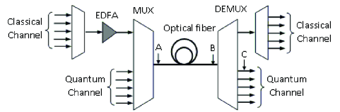
Figure 1: A typical scheme for multiplexing quantum channels with classical channels. MUX-multiplexer; DEMUX-demultiplexer; EDFA-erbium-doped fiber amplifier.

2.1 Amplified spontaneous emissions (ASE) of EDFA

It is well known that an ideal, noise-free amplifier cannot exist [29]. In the case of an optical amplifier, the fundamental noise originates from the spontaneous emission. The ASE from a practical EDFA has a broad bandwidth on the order of tens of nm which can be treated as a broadband noise source with a flat spectral power density within the spectral bandwidth of the quantum channel. We remark that a practical laser source also has a broadband noise background, which can be modeled as ASE from a virtual optical amplifier.

The average ASE photon number in one spatiotemporal mode is given by [30]

$$\langle N_{ASE}\rangle=2n_{sp}(G-1)$$ (1)

Here the factor $2$ accounts for the two orthogonal polarization modes. $G$ is the gain of the EDFA, $n_{sp}\geq 1$ is the spontaneous emission factor. If the spontaneous emission is the only noise source (no excess noise), $n_{sp}=1$.

In practice, the excess noise of an EDFA is commonly quantified by its noise figure ($NF$). In the unsaturated regime, $NF$ is related to $n_{sp}$ by [30]

$$NF=\frac{1+2n_{sp}(G-1)}{G}$$ (2)

In the high gain range ($G\gg 1$), $NF\simeq 2n_{sp}$.

Typically, the ASE power is much lower than that of the classical signal. However, its bandwidth is much broader and extends into the quantum channel. Thus the ASE will contribute to in-band noise. Fortunately, the MUX used at Alice’s side functions as a bandpass filter and can greatly suppress this in-band ASE noise. Given the cross channel isolation of the MUX is $\xi_{1}$, the in-band ASE photon number (per spatiotemporal mode) measured at the output of the MUX (point A in Fig.1) is

$$\langle N_{ASE}^{(A)}\rangle=2\xi_{1}n_{sp}(G-1)$$ (3)

Note, in this paper, we will not consider the “out-of-band” ASE noise photons, since they are typically much weaker than the classical signals themselves.

2.2 Leakage from classical channel

Although the classical signal has a different wavelength as the quantum signal, a small fraction of the classical signal will leak into the quantum channel due to the finite isolation of the DEMUX. In a BB84 QKD system, this leakage will contribute to out-of-band noise, which could be further reduced by using spectral filters at the receiver’s end. In a GMCS QKD system, this leakage contributes noise photons in “unmatched mode” of the LO.

We define the power of the classical signal output from the communication fiber as $P_{out}$ (measured at point B in Fig.1). Given the isolation of the DEMUX $\xi_{2}$, the power of the leakage signal received by Bob (measured at point C in Fig.1) is $P_{leak}=\xi_{2}P_{out}$. The average leakage photon number per second is

$$\langle N_{leak}^{(C)}\rangle=\frac{\xi_{2}P_{out}}{h\nu}$$ (4)

Here $h$ is Planck’s constant, and $\nu$ is the frequency of the classical signal.

2.3 Spontaneous anti-Stokes Raman scattering (SASRS)

As the strong classical signals propagate along the optical fiber, noise photons at different wavelength can be generated through various nonlinear optical processes. If the wavelength of the noise photons coincides with that of the quantum signal, they cannot be filtered out at the receiver’s end and will contribute to in-band noise. It has been shown that SASRS is the dominant nonlinear process when the quantum channel is placed at the shorter wavelength of the classical channel [6, 11].

The SASRS noise power within a bandwidth of $\Delta\lambda$ (measured at point B in Fig.1) is given by [6]

$$P_{SASRS}=P_{in}\beta{z}\eta_{ch}\Delta\lambda=P_{out}\beta{z}\Delta\lambda$$ (5)

Here $\beta$ is the spontaneous Raman scattering coefficient, $P_{in}$ (measured at point A in Fig.1) is the input power of the classical signal, $z$ is the fiber length and $\eta_{ch}$ is the transmittance of the optical fiber.

To estimate the noise photon number per spatiotemporal mode, we first use the relation $\nu=c/\lambda$ to determine the total mode number corresponding to a bandwidth of $\Delta\lambda$ and a time window of $\Delta t=1s$ to be $N_{mode}=|\Delta\nu\Delta t|=\frac{c}{\lambda^{2}}\Delta\lambda$. Here $c$ is the speed of light in vacuum.

Given the insertion loss of the DEMUX is $\eta_{DMU}$, the in-band SASRS photon number (per spatiotemporal mode) measured at the output of the DEMUX (point C in Fig.1) can be calculated from (5):

$$\langle N_{SASRS}^{(C)}\rangle=\frac{P_{SASRS}}{h\nu N_{mode}}\eta_{DMU}=\frac{\lambda^{3}}{hc^{2}}P_{out}\beta{z}\eta_{DMU}$$ (6)

Again, in the derivation of (6), we have used the relation $\nu=c/\lambda$.

2.4 Four-wave mixing

Four-wave mixing (FWM) is a third order nonlinear process generated by the $\chi^{(3)}$ nonlinearity of the optical fiber when two or more pumps exist. For FWM process to be efficient, phase-matching condition is required. Although FWM could be the major noise source at very short distance, it is much weaker than Raman Scattering for a practical fiber length [10]. Furthermore, FWM can be effectively suppressed by optimizing the channel configuration [10, 11] or using polarization multiplexing [10]. In this paper, we simply neglect FWM.

3 Experimental characterization of various noise sources

3.1 The performance of commercial MUX/DEMUX

Theoretical studies in Section 2 show that the noise level is dependent on the performance of MUX/DEMUX: cross-channel isolation and insertion loss.

We have tested two commercial C-band $100GHz$ MUX/DEMUX from JDSU (model number: WD1508D1B). Each of them has 8 channels with a channel separation of $0.8nm$ (or $100GHz$). The $3dB$ bandwidth of each channel is around $0.6nm$ (or $75GHz$). Based on the availability, a $1559.79nm$ fiber optic source module (ILX Lightwave, 79800D) has been used as the laser source for the classical channel. Thus, we allocate channel 2 of the MUX/DEMUX as the classical channel and channel 8 as the quantum channel. The isolation $\xi_{1}$ of MUX is determined by sending a calibrated laser beam (with a wavelength of $\lambda_{8}$) into channel 2 and measuring the optical power output from its common port. Similarly, the isolation $\xi_{2}$ of the DEMUX is determined by sending a calibrated laser beam (with a wavelength of $\lambda_{2}$) into its common port and measuring the optical power output from its channel 8. In Table 1, we list the central wavelengths ($\lambda$), insertion losses ($L$) and the cross-channel isolations ($\xi$) of two channels to be used in our experiments.

Table 1: JDSU C-band 100GHz MUX/DEMUX

Channel	$\lambda$(nm)	$L_{MUX}$(dB)	$L_{DEMUX}$(dB)	$\xi_{1}$(dB)	$\xi_{2}$(dB)
$2(classical)$	$1559.79$	$2.61$	$1.43$	$-83$	$-86$
$8(quantum)$	$1554.94$	$0.97$	$0.90$

3.2 Noise photons contributed by amplified spontaneous emissions of EDFA

The noise contributed by an EDFA has been studied in Section 2.1. However, the level of noise photon given in (3) is too low to be measured with a conventional optical power meter directly. Instead, we have performed an experiment based on a modified setup to test the validity of (1). The modified experimental setup is shown in Fig.2a. The EDFA is a commercial low noise fiber amplifier with a $NF$ of 5.5dB (PriTel, LNHPFA-30-M). A tunable optical attenuator (Att. in Fig.2) is used to simulate the transmission loss experienced by the classical signal before it reaches the multiplexer.

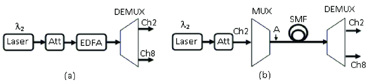
Figure 2: Experimental setups. Att-tunable optical attenuator; SMF-single mode fiber.

Referring to Fig.2a, by setting the gain of EDFA to be $G=100$, we have measured the noise power output from channel 8 to be $P_{ASE}^{(Exp)}=-25dBm$. On the other hand, from (1) the ASE photon is determined to be 351 per spatiotemporal mode. The energy of a 1550nm photon is $h\nu=1.28\times 10^{-19}J$. So, the expected noise power within $75GHz$ bandwidth (corresponding to 0.6nm) is $351\times 75\times 10^{9}\times 1.28\times 10^{-19}J=-24.7dBm$. Considering that the insertion loss of channel 8 is $0.9dB$, the expected noise power $P_{ASE}^{(Theory)}=-25.6dBm$, which reasonably matches with the experimental result $P_{ASE}^{(Exp)}$.

Next, we determine whether the background noise of the laser source itself will make a significant contribution after being amplified by the EDFA. We first determined the background noise of the laser source. By using a tunable optical attenuator, the power of the classical signal (input to the EDFA) was set to $-20dBm$. The laser background noise at $1554.94nm$ ($\lambda_{8}$) within a $0.6nm$ wavelength range (corresponding to the channel bandwidth of MUX/DEMUX) has been determined to be $-70dBm$. The number of in-band laser noise photon in one spatiotemporal mode can be determined to be around $0.01$. If the gain of EDFA is $G$, we expect that the number of the amplified laser noise photon is around $0.01G$ per spatiotemporal mode, which is significantly smaller than the number of ASE noise photon (see (1)). In this paper, we will simply neglect the contribution of the amplified laser noise.

3.3 Spontaneous anti-Stokes Raman scattering generated in SMF28 fiber

The SASRS noise photon number can be calculated from (6). The spontaneous Raman scattering coefficient $\beta$ of standard SMF28 fiber has been determined using the experimental setup shown in Fig.2b. The laser wavelength is $1559.79nm$ and the output power after the MUX (point A in Fig.2b) was set to $4dBm$. We measured the output power from channel 8 of the DEMUX for different fiber links: a $20km$ SMF28 fiber spool and a $40km$ SMF28 fiber spool. Using (5), the spontaneous Raman scattering coefficient has been determined to be $2.85\times 10^{-9}(km\cdot{nm})^{-1}$. Our result matches with the results reported in [11], which is between $2\times 10^{-9}\sim 4\times 10^{-9}(km\cdot{nm})^{-1}$ depending on the Raman shift.

In Section 4, we will calculate the secure key rates of both the decoy state BB84 protocol and the GMCS QKD protocol in a typical DWDM configuration as shown in Fig.1. The simulation parameters are summarized in Table 2. To make our simulation results more applicable, some parameters in Table 2, such as $NF$, $\eta_{MUX}$, $\eta_{DMU}$, $\xi_{1}$ and $\xi_{2}$, have been chosen to be slightly worse than the experimental values on purpose. Since the spontaneous Raman scattering coefficient $\beta$ is wavelength dependent, we have assumed the worst case of $\beta=4\times 10^{-9}(km\cdot{nm})^{-1}$ [11]. The parameters of the GMCS QKD system are from [32].

Table 2: Simulation Parameters

Parameter	Value
NF (Noise figure of EDFA)	4 (or 6dB)
$\alpha$ (Fiber attenuation coefficient)	0.21dB/km
$\beta$ (Spontaneous Raman scattering coefficient)	$4\times 10^{-9}/(km\cdot nm)$
$\eta_{MUX}$ (Transmittance of MUX)	0.71 (or 1.5dB loss)
$\eta_{DMU}$ (Transmittance of DEMUX)	0.71 (or 1.5dB loss)
$\xi_{1}$ (Isolation of MUX)	$10^{-8}$ (or -80dB)
$\xi_{2}$ (Isolation of DEMUX)	$10^{-8}$ (or -80dB)
$\Delta{\nu}$ (3dB channel bandwidth)	75GHz
$\Delta{t}$ (Gating window of SPD)	1ns
$V_{A}$ (Modulation variance, GMCS)	10
$\eta_{Bob}$ (Transmittance of Bob’s system, GMCS)	0.6
$\epsilon_{0}$ (GMCS parameter)	0.01
$\upsilon_{el}$ (GMCS parameter)	0.01
$\gamma$ (Efficiency of reverse reconciliation algorithm)	0.9

4 System comparison: single-photon detection scheme vs. homodyne detection scheme

4.1 A single-photon detection based scheme: decoy state BB84 QKD with a weak coherent source

Refer to Fig.1, in the BB84 QKD protocol, the quantum signal is at the single photon level, so the crosstalk between the quantum channels is negligible. We consider the simplest case where only one classical channel (at a longer wavelength and non-adjacent channel) is multiplexed with quantum channels.

In the BB84 QKD, single photon detectors are employed to detect quantum signals. At telecom wavelength, InGaAs APDs working at the gated Geiger mode are frequently used as SPDs. In this case, the gating window of the SPD functions as a temporal filter, which can reduce the effective noise photon number. For other non-gated detection systems, this noise reduction can be achieved by introducing an adjustable detection time window.

Given the channel bandwidth $\Delta{\nu}$ of MUX/DEMUX and the gating window $\Delta{t}$ of the SPD, the total mode number of the noise photons which can be detected by the SPD is

$$N_{Mod}=\Delta{\nu}\Delta{t}$$ (7)

The number of noise photons arrived at Bob (point C in Fig.1) within one gating window is

$$\langle N_{SPD}^{tot}\rangle=N_{Mod}\eta_{ch}\eta_{DMU}\langle N_{ASE}^{(A)}\rangle+\langle N_{leak}^{(C)}\rangle\Delta{t}+N_{Mod}\langle N_{SASRS}^{(C)}\rangle$$ (8)

Here $\langle N_{ASE}^{(A)}\rangle$, $\langle N_{leak}^{(C)}\rangle$ and $\langle N_{SASRS}^{(C)}\rangle$ are determined from equations (3), (4) and (6) respectively. At the RHS of (8), the superscripts are used to refer to the location where noise photons are evaluated.

The gain of EDFA is adjusted with the channel transmittance $\eta_{ch}$ to maintain a constant $P_{out}$ (point B in Fig.1) of the classical channel. In this paper, we assume $G=100/\eta_{ch}$.

Using (3-8), we calculated the number of noise photons $\langle N_{SPD}^{tot}\rangle$ as a function of the fiber length. We have assumed that $P_{out}=0dBm$ and $G=100/\eta_{ch}$. Other simulation parameters are summarized in Table 2. Fig.3 shows the simulation results: at short distances, the main contribution of noise photons is the leakage from the classical channel; while at long distances, most of the noise photons are from SASRS. Noise contributed by the EDFA is negligible.

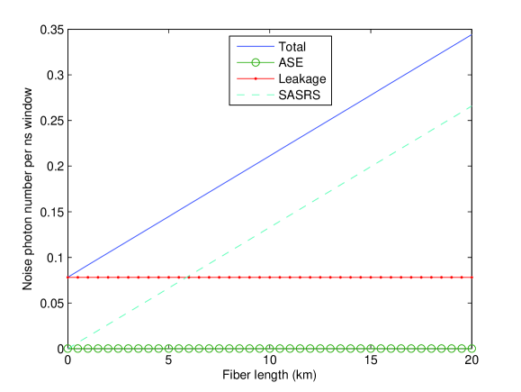
Figure 3: The number of noise photons arrived within 1ns gating window of SPD. The power of the classical signal output from the communication fiber is assumed to be $P_{out}=0dBm$ regardless of the fiber length. The EDFA gain $G=100/\eta_{ch}$. Other simulation parameters are summarized in Table 2.

In the BB84 QKD system, noise photons trigger random detection events and contribute to quantum bit errors. This contribution can be included in the total background count rate:

$$Y_{0}=Y_{0}^{0}+\eta_{Bob}\langle N_{SPD}^{tot}\rangle$$ (9)

Here $Y_{0}^{0}$ is the background rate of the original QKD system. The error rate of background counts is assumed to be $e_{0}=0.5$.

We assume that Alice and Bob perform perfect decoy state BB84 protocol with infinite decoy states. In the asymptotic limit of infinitely many signals sent by Alice, the secure key rate (per signal sent by Alice) is given by [19]

$$R=\frac{1}{2}[Q_{1}-f(E_{\mu})Q_{\mu}H_{2}(E_{\mu})-Q_{1}H_{2}(e_{1})].$$ (10)

Here $\mu$ is the expected photon number of the signal state, $Q_{\mu}$, $E_{\mu}$ are the gain and the overall quantum bit error rate (QBER) of signal states, while $Q_{1}$, $e_{1}$ are the gain and the QBER of single-photon components, $f\geq 1$ is the inefficiency factor of the error correction algorithm. The estimated values of the above parameters are given by [15]

$$Q_{\mu}=Y_{0}+1-e^{-\eta\mu}$$ (11)

$$E_{\mu}=[e_{0}Y_{0}+e_{det}(1-e^{-\eta\mu})]/Q_{\mu}$$ (12)

$$Q_{1}=(Y_{0}+\eta)\mu e^{-\mu}$$ (13)

$$e_{1}=(e_{0}Y_{0}+e_{det}\eta)\mu e^{-\mu}/Q_{1}$$ (14)

Here $e_{det}$ is the probability that a single photon hits the wrong detector when Alice and Bob choose the same basis. $\eta=\eta_{ch}\eta_{DMU}\eta_{Bob}$ is the overall efficiency, where $\eta_{Bob}$ is the efficiency of Bob’s system.

Given the noise photons shown in Fig.3, we calculated the secure key rate of the decoy BB84 QKD system using (9-14). The simulation parameters are chosen to be [11] $e_{det}=0.003$, $Y_{0}^{0}=5\times 10^{-6}$, $\eta_{Bob}=0.038$ and $f=1.22$. The simulation results show that no secure key can be generated at any distance. We remark that the simulation results are not sensitive to the actual values of $e_{det}$ and $Y_{0}^{0}$ since the quantum bit errors are mainly contributed by the noise photons due to multiplexing.

4.2 A homodyne detection based scheme: GMCS QKD

The GMCS QKD has drawn a lot of attention for its potential high secure key rate, especially at relatively short distances [17, 26, 31, 32]. In this protocol, instead of performing single photon detection, Bob measures either the phase quadrature or the amplitude quadrature of a weak coherent state by using a homodyne detector. The strong LO used in homodyne detection acts as a “mode” filter: only noise photons in the same spatiotemporal and polarization mode as the LO can be detected, while noise photons in unmatched modes will be effectively suppressed. However, if the number of noise photons in unmatched modes is comparable to the photon number of the LO, their contributions cannot be neglected [12].

Refer to Fig.1, in the GMCS QKD protocol, the optical power of each quantum channel is mainly determined by the operation rate and the average photon number of LO. Given a 1MHz operation rate and a LO of $10^{8}$ photons per pulse, the optical power of each quantum channel is around $-19dBm$, which is significantly lower than the average power of the classical signal ($0dBm$). Here, we simply neglect the crosstalk between quantum channels. If a pair of QKD users can access multiple quantum channels, the achievable secure key rate will scale with the channel number. We further assume that all the classical channels are at longer wavelengths of the QKD signals and the total noise contributed by all the classical channels is simply a summation of the noise contributed by each channel.

4.2.1 Noise photons in matched mode

Noise photons in the same spatiotemporal and polarization mode as the LO are contributed by in-band ASE and SASRS. The number of noise photons in matched mode arrived at Bob (point C in Fig.1) is

$$\langle N_{GMCS}^{in}\rangle=\frac{1}{2}m(\eta_{ch}\eta_{DMU}\langle N_{ASE}^{(A)}\rangle+\langle N_{SASRS}^{(C)}\rangle)$$ (15)

Here, the factor 1/2 is due to the polarization selection of the LO, $m$ is the number of classical channel, $\langle N_{ASE}^{(A)}\rangle$ and $\langle N_{SASRS}^{(C)}\rangle$ are determined by (3) and (6).

Both the ASE and the SASRS can be modeled as output from a chaotic source with Bose$\--$Einstein photon statistics [33, 34]. For a chaotic source with an average photon number of $\langle n\rangle$, the quadrature variances in shot noise unit are given by [35]:

$$(\Delta X)^{2}=(\Delta Y)^{2}=2\langle n\rangle+1$$ (16)

Using (15) and (16), the “excess noise” contributed by noise photons in matched mode is given by

$$\varepsilon_{in}=2\eta_{Bob}\langle N_{GMCS}^{in}\rangle$$ (17)

4.2.2 Noise photons in unmatched modes

In the normal working condition, the pulse width of the LO is significantly smaller than the integration time of the homodyne detector. The latter is determined by the bandwith $\Delta f$ of the homodyne detector and can be estimated by $\Delta T=\frac{1}{2\pi\Delta{f}}$. Similar to (8), which gives the noise photon number within one gating window $\Delta{t}$ of the SPD, the number of noise photons in “unmatched modes” measured at Bob (point C in Fig.1) within the time window of $\Delta{T}$ is given by

$$\langle N_{GMCS}^{out}\rangle=\frac{\Delta{T}}{\Delta{t}}\langle N_{SPD}^{tot}\rangle$$ (18)

Again, we model the noise photons in unmatched modes as the output of a chaotic source. The photon number variance of a single mode chaotic light is given by [35]:

$$(\Delta{n})^{2}=\langle n\rangle^{2}+\langle n\rangle$$ (19)

where $\langle n\rangle$ is the average photon number.

However, the integration time $\Delta T$ of the homodyne detector is normally much larger than the coherence time $\tau_{c}$ of the noise photon [36]. Under this condition, the photon number statistics follows Poisson distribution [37]. Thus the “excess noise” contributed by noise photons in unmatched modes is

$$\varepsilon_{out}=\eta_{Bob}\langle N_{GMCS}^{out}\rangle/\langle n_{LO}\rangle$$ (20)

Note in (20), we have added in a factor of $1/\langle n_{LO}\rangle$ to express $\varepsilon_{out}$ in shot noise unit, where $\langle n_{LO}\rangle$ is the average photon number of the LO.

For example, if we assume that the bandwidth of the homodyne detector is $\Delta{f}=1MHz$, then $\Delta{T}=0.16\mu s$. Since we have assumed that the gating window of the SPD is $\Delta{t}=1ns$, from (18), $\langle N_{GMCS}^{out}\rangle=160\times\langle N_{SPD}^{tot}\rangle$. Based on the results in Fig.3, we expect that the total number of noise photons in unmatched modes $\langle N_{GMCS}^{out}\rangle$ is in the order of $10^{2}$. If we further assume that $\langle n_{LO}\rangle=10^{8}$, then $\varepsilon_{out}$ is in the order of $10^{-6}$, which is negligible. In this paper, we will neglect the contribution from photons in unmatched modes.

4.2.3 Secure key rate of the GMCS QKD

Under the “realistic model” [17], the secure key rate (per signal sent by Alice) of the GMCS QKD with “reverse reconciliation” protocol is given by [32]

$$\Delta I=\gamma I_{AB}-\chi_{BE}$$ (21)

where $\gamma$ is the efficiency of the reverse reconciliation algorithm, and

$$I_{AB}=\frac{1}{2}\log_{2}[(V+\chi_{tot})/(1+\chi_{tot})]$$ (22)

$$\chi_{BE}=\Theta(\frac{\sigma_{1}-1}{2})+\Theta(\frac{\sigma_{2}-1}{2})-\Theta(\frac{\sigma_{3}-1}{2})-\Theta(\frac{\sigma_{4}-1}{2})$$ (23)

with $\Theta(x)=(x+1)log_{2}(x+1)-xlog_{2}x$; $\chi_{tot}=\chi_{line}+\chi_{hom}/\eta_{ch}$; $\chi_{line}=1/\eta_{ch}-1+\epsilon$; $\chi_{hom}=(1+\upsilon_{el})/\eta^{\prime}-1$; $\sigma^{2}_{1,2}=\frac{1}{2}(A\pm\sqrt{A^{2}-4B)}$; $\sigma^{2}_{3,4}=\frac{1}{2}(C\pm\sqrt{C^{2}-4D)}$; $A=V^{2}(1-2\eta_{ch})+2\eta_{ch}+\eta^{2}_{ch}(V+\chi_{line})^{2}$; $B=\eta_{ch}^{2}(V\chi_{line}+1)^{2}$; $C=\frac{V\sqrt{B}+\eta_{ch}(V+\chi_{line})+A\chi_{hom}}{\eta_{ch}(V+\chi_{tot})}$; $D=\sqrt{B}\frac{V+\sqrt{B}\chi_{hom}}{\eta_{ch}(V+\chi_{tot})}$. Here, $V=V_{A}+1$ is the quadrature variance of the coherent state prepared by Alice. $\eta^{\prime}=\eta_{DMU}\eta_{Bob}$ is the equivalent efficiency of Bob’s system. $\epsilon$ denotes noise contribution from outside of Bob’s system, which can be further separated into two terms:

$$\epsilon=\epsilon_{0}+\frac{\varepsilon_{in}}{\eta_{ch}\eta_{DMU}\eta_{Bob}}$$ (24)

Here $\epsilon_{0}$ is contributed by the original GMCS QKD system. $\varepsilon_{in}$ is the excess noise due to multiplexing with the classical channels and can be determined from (17). Note that $\varepsilon_{in}$ is determined at Bob’s side, while $\epsilon$ and $\epsilon_{0}$ are referred to input.

We have performed numerical simulations using parameters in Table 2 and the results are shown in Fig.4. In Fig.4, the secure key rates have been calculated under 5 different conditions: (1) No classical signal; (2) One non-adjacent classical channel ($0dBm$); (3) One adjacent classical channel ($0dBm$); (4) 38 non-adjacent classical channels ($0dBm$ per channel); (5) One non-adjacent classical channel ($0dBm$) with our 100MHz homodyne detector (see details in Section 4.2.4). In all the above cases, the optical power is defined at the output of the communication channel (point B in Fig.1). Note under condition (3), we have assumed that the isolation of MUX/DEMUX between adjacent channels is $-40dB$, which is achievable with commercial products . From Fig.4, it is possible to multiplex the GMCS QKD with a $0dBm$ classical channel without significantly reducing its performance. Even multiplexed with 38 classical channels ($0dBm$ power each channel), the GMCS QKD still has a secure distance around $10km$. We remark that Eq. (23) was derived from the realistic model [17], where Eve cannot take advantages of noise contributed by Bob’s system [38]. In the more conservative “general model” [17], where Eve can control losses and noise in Bob’s system, the secure distance is much shorter [31]. In practice, the realistic model has been commonly used [26, 31, 32].

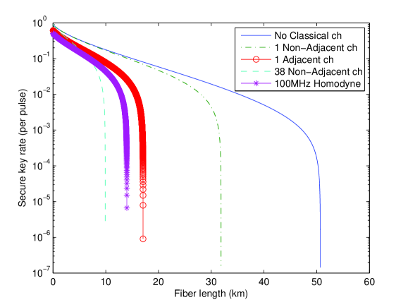
Figure 4: The secure key rate of the GMCS QKD under the “realistic model”. The secure key rates have been calculated under 5 different conditions: (1) No classical signal; (2) One non-adjacent classical channel ($0dBm$); (3) One adjacent classical channel ($0dBm$); (4) 38 non-adjacent classical channels ($0dBm$ per channel); (5) One non-adjacent classical channel ($0dBm$) with our 100MHz homodyne detector (see details in Section 4.2.4). Note under condition (3), we have assumed that the isolation of MUX/DEMUX between adjacent channels is $-40dB$. Other parameters are summarized in Table II.

4.2.4 Preliminary experimental results with a 100MHz homodyne detector

Recently, we have developed a $100MHz$ bandwidth shot-noise limited optical homodyne detector [39]. With a LO photon number of $4\times 10^{8}$, the electrical noise of the homodyne detector is $10dB$ below the shot noise.

The noise photons output from the DWDM system (point C in Fig.1) has been fed into the 100MHz homodyne detector. The fiber length used in this experiment is $20km$. The variance of the output of the homodyne detector has been measured as a function of the LO power under three conditions: (1) No classical channel; (2) One classical channel ($P_{out}=3.4dBm,G=100/\eta_{ch}$) is placed at channel 2, channel 8 is used as the quantum channel; (3) One classical channel ($P_{out}=3.4dBm,G=100/\eta_{ch}$) is placed at channel 2, channel 1 is used as the quantum channel. Note under condition (3), the quantum channel is placed at the adjacent channel of the classical channel. Under both condition (2) and (3), the additional excess noise due to multiplexing has been estimated from (17) to be less than 0.01 (in shot noise unit). On the other hand, the measurement uncertainty of our homodyne detection system on determining the noise variance has been measured to be $\varsigma=0.024$ (in shot noise unit) . As shown in Fig.5, there is no observable difference among the 3 measurement results. To determine the magnitude of multiplexing noise more accurately, the measurement accuracy of the homodyne detector has to be further improved.

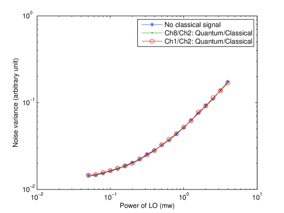
Figure 5: Experimental results with a 100MHz homodyne detector. The total variance of the output of the homodyne detector has been measured as a function of the LO power under three conditions: (1) No classical channel; (2) One classical channel ($P_{out}=3.4dBm,G=100/\eta_{ch}$) is placed at channel 2, channel 8 is used as the quantum channel; (3) One classical channel ($P_{out}=3.4dBm,G=100/\eta_{ch}$) is placed at channel 2, channel 1 is used as the quantum channel. The fiber length is 20km. From the experimental results, there is no observable difference among the 3 curves.

This raises up a question about how to apply the realistic model using this homodyne detector, since Bob has to estimate the excess noise from his system and the one from outside separately. To determine the excess noise contribution from outside of Bob’s system ($\epsilon$), one common way is to subtract the total observed noise by the vacuum noise associated with the transmission efficiency and the electrical noise ($\upsilon_{el}$) contributed by Bob’s homodyne detector. Obviously, the minimal $\epsilon$ resolvable by this method is determined by the measurement uncertainty $\varsigma$ of the homodyne detector .

Note that the simulation results shown in Fig.4 (except the one acquired under condition (5)) are based on parameters of the GMCS QKD system from [32], where a low speed (1MHz bandwidth) and low electronic noise (20dB below the shot noise) homodyne detector was employed. So we have assumed that the measurement uncertainty of the homodyne detector is small enough to resolve the excess noise due to multiplexing. In our preliminary experiment, however, the homodyne detector has a larger bandwidth (100MHz) but also higher electronic noise (10dB below the shot noise). As a conservative estimation of $\epsilon$, we could replace (24) by

$$\epsilon=\epsilon_{0}+\frac{\varepsilon_{in}}{\eta_{ch}\eta_{DMU}\eta_{Bob}}+\frac{\varsigma}{\eta_{ch}\eta_{DMU}\eta_{Bob}}$$ (25)

Using (25), we have performed numerical simulations based on parameters of the 100MHz homodyne detector: $\upsilon_{el}=0.1$ and $\varsigma=0.024$. Other parameters are shown in Table 2. We have assumed that one non-adjacent classical channel ($0dBm$) is multiplexed with the quantum channel. The simulation result is also shown in Fig.4 (under condition (5)) where the secure distance is about 14km. Note that the secure key rate under condition (5) is significantly lower than that under condition (2). This is mainly due to the larger measurement uncertainty of the 100MHz homodyne detector. To apply the realistic model more efficiently, we may need a more accurate way than the one given by (25) to estimate $\epsilon$.

We would like to end this section with a few comments on the realistic model adopted in the GMCS QKD. In all the security proofs mentioned in Section 1, one underlying assumption is that both Alice and Bob’s QKD systems are fabricated by trusted vendors and these devices are placed inside Alice and Bob’s local secure stations which cannot be accessed by Eve. So it might be reasonable to assume that Eve cannot control the internal parameters of Bob’s system (the realistic model). However, to justify the above assumption in practice, we may need to develop special techniques to estimate each system parameter accurately without compromising the security of the QKD system. As we have discussed in Section 1, to apply the security proof of an idealized QKD protocol to a practical QKD system, all the underlying assumptions and implementation details have to be studied carefully.

5 Conclusion

In summary, we have studied the feasibility of conducting QKD together with classical communication through the same fiber by employing C-band DWDM technology. The impact of the classical channel to the quantum channel has been investigated for both QKD based on single photon detection and QKD based on homodyne detection. Our studies show that the latter can tolerate a much higher level of contamination from the classical channel than the former. We have performed simulations based on both the decoy BB84 QKD protocol and the GMCS QKD protocol. With commercial DWDM components, our simulation results show that it is possible to multiplex the GMCS QKD with a $0dBm$ classical channel without significantly reducing its performance. Even multiplexed with $38$ classical channels ($0dBm$ power each channel), the GMCS QKD still has a secure distance around $10km$.

Although the LO is assumed to be a single mode coherent state in this paper (which is not difficult to achieve in practice), it doesn’t have to be transform-limited.

The noise photons in the BB84 QKD system could be further reduced by employing narrow spectral filter and temporal filter. For example, in [11], a $45pm$ spectral filter has been employed to further cut off noise. In [40], the author suggested to use an additional optical gate to further suppress noise photons in time domain. In principle, it is possible to selectively detect photons in only one spatiotemporal mode by using an optimal combination of spectral and temporal filters [41]. However, in practice, both the spectral filter with extremely narrow bandwidth and the temporal filter with extremely narrow time window are difficult to fabricate and lossy as well as unstable (subject to minute changes in temperature, pressure, etc.). Furthermore, Alice’s signal has to be transform-limited to pass through these filters effectively. This also requires careful dispersion management in the communication channel.

Financial support from CFI, CIPI, the CRC program, CIFAR, MITACS, NSERC, OIT, and QuantumWorks is gratefully acknowledged.

References

References

- [1] C. H. Bennett, G. Brassard, Proceedings of IEEE International Conference on Computers, Systems, and Signal Processing, (IEEE, 1984), pp. 175-179.
- [2] A. K. Ekert, Phys. Rev. Lett. 67 661 (1991).
- [3] C. Elliott, New J. Phys. 4 46.1-46.12 (2002).
- [4] V. Fernandez, R. J. Collins, K. J. Gordon, P. D. Townsend, and G. S. Buller, IEEE J. Quantum Electron. 43 130 (2007).
- [5] M. Peev, et al, New J. Phys. 11 075001 (2009).
- [6] T. E. Chapuran, P. Toliver, N. A. Peters, J. Jackel, M. S. Goodman, R. J. Runser, S. R. McNown, N. Dallmann, R. J. Hughes, K. P. McCabe, J. E. Nordholt, C. G. Peterson, K. T. Tyagi, L. Mercer and H. Dardy, New J. Phys. 11 105001 (2009).
- [7] P. D. Townsend, Electron. Lett. 33 188 (1997).
- [8] T. J. Xia, D. Z. Chen, G. A. Wellbrock, A. Zavriyev, A. C. Beal, and K. M. Lee, “In-Band Quantum Key Distribution (QKD) on Fiber Populated by High-Speed Classical Data Channels,” in Optical Fiber Communication Conference and Exposition and The National Fiber Optic Engineers Conference, Technical Digest (CD) (Optical Society of America, 2006), paper OTuJ7.
- [9] G. B. Xavier, G. V. de Faria, G. P. Temporao and J. P. von der Weid, “Scattering Effects on QKD Employing Simultaneous Classical and Quantum Channels in Telecom Optical Fibers in the C-band Conference Information”, QUANTUM COMMUNICATION, MEASUREMENT AND COMPUTING (QCMC) Book Series: AIP Conference Proceedings 1110 327-330 (2009).
- [10] N. A. Peters, P. Toliver, T. E. Chapuran, R. J. Runser, S. R. McNown, C. G. Peterson, D. Rosenberg, N. Dallmann, R. J. Hughes, K. P. McCabe, J. E. Nordholt and K. T. Tyagi, New J. Phys. 11 045012 (2009).
- [11] P. Eraerds, N. Walenta, M. Legré, N. Gisin, and H. Zbinden, arXiv:0912.1798v1 (2009).
- [12] M. G. Raymer, J. Cooper, and H. J. Carmichael, M. Beck, D. T. Smithey, J. Opt. Soc. Am. B 12 1801 (1995).
- [13] D. Elser, T. Bartley, B. Heim, Ch. Wittmann, D. Sych, and G. Leuchs, New J. Phys. 11 045014 (2009).
- [14] W.-Y. Hwang, Phys. Rev. Lett. 91, 057901 (2003); H.-K. Lo, in Proceedings of IEEE ISIT 2004, p. 137; H.-K. Lo, X. Ma, K. Chen, Phys. Rev. Lett. 94 230504 (2005); X. -B. Wang, Phys. Rev. Lett. 94 230503 (2005).
- [15] X. Ma, B. Qi, Y. Zhao, and H.-K. Lo, Phys. Rev. A 72 012326 (2005).
- [16] Y. Zhao, B. Qi, X. Ma, L. Qian, and H.-K. Lo, Phys. Rev. Lett. 96 070502 (2006).
- [17] F. Grosshans, G. V. Assche, J. Wenger, R. Brouri, N. J. Cerf, and P. Grangier, Nature 421 238 (2003).
- [18] D. Mayers, J. of ACM 48 351 (2001); H.-K. Lo and H. F. Chau, Science 283 2050 (1999); P. Shor and J. Preskill, Phys. Rev. Lett. 85 441 (2000).
- [19] D. Gottesman, H.-K. Lo, N. Lütkenhaus, and J. Preskill, Quantum Inf. Comput. 4 325 (2004).
- [20] H. Inamori, N. Lütkenhaus, and D. Mayers, European Physical Journal D 41 599 (2007).
- [21] C.-H. F. Fung, K. Tamaki, B. Qi, H.-K. Lo, and X. Ma, Quant. Inf. and Comput. 9 131 (2009).
- [22] F. Grosshans, and P. Grangier, Phys. Rev. Lett. 88 057902 (2002).
- [23] F. Grosshans, and N. J. Cerf, Phys. Rev. Lett. 92 047905 (2004).
- [24] M. Navascues, F. Grosshans, and A. Acin, Phys. Rev. Lett. 97 190502 (2006).
- [25] R. Garcia-Patron, and N. J. Cerf, Phys. Rev. Lett. 97 190503 (2006).
- [26] J. Lodewyck, M. Bloch, R. García-Patrón, S. Fossier, E. Karpov, E. Diamanti, T. Debuisschert, N. J. Cerf, R. Tualle-Brouri, S. W. McLaughlin, and P. Grangier, Phys. Rev. A 76 042305 (2007).
- [27] R. Renner, and J. I. Cirac, Phys. Rev. Lett. 102 110504 (2009); A. Leverrier, E. Karpov, P. Grangier, and N. J. Cerf, New J. Phys. 11 115009 (2009); Y. B. Zhao, Z. F. Han, and G. C. Guo, arXiv:0809.2683v2 (2008).
- [28] T. Hirano, H. Yamanaka, M. Ashikaga, T. Konishi, and R. Namiki, Phys. Rev. A 68 042331 (2003).
- [29] C. M. Caves, Phys. Rev. D 26 1817 (1982).
- [30] E. Desurvire, Erbium-Doped Fiber Amplifiers (Wiley, New York,1994).
- [31] B. Qi, L.-L. Huang, L. Qian, H.-K. Lo, Phys. Rev. A 76 052323 (2007).
- [32] S. Fossier, E. Diamanti, T. Debuisschert, A. Villing, R. Tualle-Brouri, and P. Grangier, New J. Phys. 11 045023 (2009).
- [33] P. Voss, M. Vasilyev, D. Levandovsky, T.-G. Noh, and P. Kumar, Photon. Technol. Lett. 12, 1340 (2000).
- [34] P. Voss, R. Tang, and P. Kumar, Opt. Lett. 28, 549 (2003).
- [35] R. Loudon, The quantum theory of light, 6th ed, chapter 5.4. (Oxford University Press, 2000).
- [36] For example, if we assume that the bandwidth of the homodyne detector is , then the integration time . The coherence time of the SASRS noise is determied by the bandwidth of the DEMUX as . Using , we get . The coherence time of the classical signal depends on both the laser source and the data rate. If we assume the data rate of the classical channel is 10GHz, then the coherence time of the classical signal is less than 100ps.
- [37] P. W. Milonni and J. H. Eberly, Lasers, page 571. (New York: Wiley, 1988).
- [38] In the GMCS QKD, Alice and Bob estimate Eve’s information from the observed excess noise and other system parameters. A higher noise indicates more information leakage and thus a lower secure key rate. In practice, it may be reasonable to assume that Eve cannot control devices inside Bob’s system. Under this “realistic model”, noise inside and outside of Bob’s system are treated differently: while part of the excess noise (e.g., due to imperfections outside of Bob’s system) might originate from Eve’s attack, the noise contributed by Bob’s devices is an intrinsic parameter of the QKD system of which Eve has no control. Comparing with the more conservative “general model” where Eve can control losses and noise in Bob’s system, the realistic model allows Alice and Bob to acquire a tighter bound on Eve’s information and thus yields a higher secure key rate.
- [39] Y.-M. Chi, B. Qi, W. Zhu, L. Qian, H.-K. Lo, S.-H. Youn, A. I. Lvovsky and L. Tian, arXiv:1006.1257 (2010).
- [40] M. J. LaGasse, United States Patent Application, 20080273703.
- [41] B. Qi and L. Qian, Opt. Lett. 32, 418 (2007).