Spin-Orbit Effects in Carbon-Nanotube Double Quantum Dots

Abstract

We study the energy spectrum of symmetric double quantum dots in narrow-gap carbon nanotubes with one and two electrostatically confined electrons in the presence of spin-orbit and Coulomb interactions. Compared to GaAs quantum dots, the spectrum exhibits a much richer structure because of the spin-orbit interaction that couples the electron’s isospin to its real spin through two independent coupling constants. In a single dot, both constants combine to split the spectrum into two Kramers doublets, while the antisymmetric constant solely controls the difference in the tunneling rates of the Kramers doublets between the dots. For the two-electron regime, the detailed structure of the spin-orbit split energy spectrum is investigated as a function of detuning between the quantum dots in a $22$-dimensional Hilbert space within the framework of a single-longitudinal-mode model. We find a competing effect of the tunneling and Coulomb interaction. The former favors a left-right symmetric two-particle ground state, while in the regime where the Coulomb interaction dominates over tunneling, a left-right antisymmetric ground state is found. As a result, ground states on both sides of the $(11)$-$(02)$ degeneracy point may possess opposite left-right symmetry, and the electron dynamics when tuning the system from one side of the $(11)$-$(02)$ degeneracy point to the other is controlled by three selection rules (in spin, isospin, and left-right symmetry). We discuss implications for the spin-dephasing and Pauli blockade experiments.

I Introduction

Coherent control over the charge and/or the spin of an electron or hole is a key ingredient for quantum computation or spintronic devices. It is of importance to have coupled two level systems (qubits) that can be controlled and manipulated efficiently without loss of the stored information. A promising candidate and natural two-state system for a robust qubit is the spin of an electron. Coherent manipulation as well as preparation and read-out of a single confined spin in few electron semiconductor quantum dot (QD) systems have been demonstrated, see Refs. Hanson, and Petta, and references therein.

Spin qubits in carbon nanotubesIijima ; Kuemmeth2 (CNT) are believed to be even more robust due to the absence of hyperfine coupling in ${}^{12}C$.Churchill2 This is in contrast to GaAs QDs where the phase coherence suffers from hyperfine coupling due to the nuclei of the host crystal. However, CNTs pose other challenges and complications. First, few electron QDs are not easily fabricated and, secondly, the isospin degree of freedom present in the honeycomb carbon lattice provides another quantum two level system that must be included in the analysis.

The band structure of electrons in nanotubes can be understood starting from that of graphene,Dresselhaus ; Castro which has a linear dispersion relation similar to massless Dirac-Weyl fermions. Graphene is a zero gap semiconductor, but when the graphene sheet is rolled to form a nanotube, the quantization condition for nanotubes leads to metallic or semiconducting behavior, depending on chirality. Ando ; Roche The curved geometry creates a mass term in the Dirac spectrum and thus a bandgap even for the nominally metallic tubes.Kanecurv ; Kleiner ; Mintmire ; Hamada ; Saito1 This bandgap allows for electrostatic confinement of electrons and creation of few electron QDs, otherwise not possible due to the Klein paradox.Kouwenhoven Recent experiments have shown that it is indeed possible to confine electrons in single Jarillo ; Minot ; Kuemmeth ; Leturcq and double quantum dots (DQD) in a CNT by means of electrostatic gates in cleanly grown small bandgap nanotubes.Churchill ; Kouwenhoven ; Churchill2 The present study is motivated by these experimental results.

In the recently investigated few-electron nanotube QDs, the four-fold degeneracy due to the spin and isospin degrees of freedom is split by SO coupling, giving rise to a coupling of spin and isospin degrees of freedom. In plane graphene, spin-orbit (SO) coupling (being a relativistic effect) of its $\pi$-electrons is of dozens of $\mu$eV only MacDonald ; Yao ; Boettger ; Gmitra and therefore of minor importance. The curved geometry of nanotubes induces SO coupling on the order of $10^{-1}$ meV among the single particle levels of the electrons.Kuemmeth While the curvature-induced SO coupling was envisioned previously for semiconductors,Entin ; Bulgakov for nanotubes it is the dominant mechanism. It was Ando AndoSO and others DeMartino ; Chico2004 who developed the first theories of SO coupling in nanotubes. More recent theoretical investigations extended this work by including the $\sigma$- and $\pi$- bands in full as well as the curved bonds between neighboring atoms.HH ; Izumida ; Jeong ; Chico Lowest order perturbation theory shows that the SO coupling is inversely proportional to the radius of curvature and originates from the intra-atomic SO coupling in a carbon atom. Even though this is a weak coupling compared to heavier atoms, the combined effect of curvature and intra-atomic SO coupling splits a four-fold degenerate level into two Kramers doublets by a fraction of a meV. The demonstration of electrostatically confined particles in CNT-QDs in the presence of SO coupling Kuemmeth ; Churchill has motivated recent theoretical investigations. The single electron QD setup and in particular the influence of the electron-phonon coupling on the decoherence are subjects of a work by Bulaev et. al. Bulaev The two-particle problem has been studied numerically in Refs. Wunsch, and Rontani, for a hard wall and a harmonic potential, respectively. Furthermore, hyperfine interactions and their consequences for Pauli blockade have been discussed. Fischer ; Burkard

Here, we present a theory of the energy spectrum for a CNT-DQD in the presence of SO coupling in the envelope function formalism within an exact diagonalization scheme. The system is described by three quantum numbers [spin $s$, isospin $\tau$, and left and right dots ($L/R$)], each taking two values, and by the discrete and continuum spectra of the longitudinal motion. Depending on the specific parameter values of the DQD that vary in a wide range, two electrons confined in a DQD find themselves in rather different regimes. In this article, we concentrate on coated narrow-gap nanotubes of the kind investigated in Refs. Churchill2, and Churchill, that seem well suited for spintronic applications. In such DQDs, a small electron mass $m^{*}$ increases the separation between the levels of longitudinal quantization, while a high dielectric constant $\kappa\sim 10$ suppresses the Coulomb repulsion, which would otherwise result in level mixing. Restricting ourselves with the lowest longitudinal mode, we concentrate instead on the detailed structure of the energy spectrum emerging from the spin-isospin coupling, and the dependence of the interdot tunneling and Coulomb energies on the symmetry of wave functions and SO coupling. However, we stop short of discussing the influence of phonon and hyperfine couplings as well as the scattering between different isospin states.Burkard It should be mentioned that similar physics occurs in silicon double quantum dots where, however, the valley degeneracy is usually broken and spin-orbit interaction does not play an important role.Culcer

To set up our model calculation, we use the well-established model for $p_{z}$-orbitals of graphene to describe electrons in a nanotube. The DQD confinement is modeled by a double square-well potential along the axial direction of the nanotube. We take into account SO coupling effects on the single particle levels and discuss their influence on the energy spectrum in the presence of an axial magnetic field $B$. In the framework of a single-mode approximation, and using the eight-function basis $(8=2\times 2\times 2)$ of single-electron states, we present a symmetry classification of the eigenstates of a two-electron symmetric DQD in its 22-dimensional Hilbert space. We find its energy spectrum numerically for the comparable values of the tunneling integral, the Coulomb interaction and the SO splitting. Our main results include the detuning dependence of the spectrum and the effect of a magnetic field lifting all spectrum degeneracies. Finally, we discuss challenges and opportunities for experimental studies.

The structure of the article is as follows. After we have summarized the physical properties of a single electron in a nanotube in Sec. II.1, we turn in Sec. II.2 to the model of an electrostatically generated DQD and solve the eigenvalue problem for a DQD with a square-well potential. We clarify the effect of two SO coupling constants, $\Delta_{0}$ and $\Delta_{1}$, on the energy splitting between the Kramers doublets and on the tunneling integral. Sec. III presents the symmetry classification of the two-electron wave functions as well as a description of the techniques used for calculating Coulomb integrals on SO modified wave functions, and the effect of SO coupling on Coulomb integrals as well as their $B$-dependence. In Sec. IV we present our main results on the energy spectrum of a two-electron DQD as a function of detuning and its transformation when a magnetic field is applied. Summary and discussion are presented in Sec. V.

II Model

II.1 Single electron in a nanotube

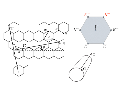
Figure 1: Sketch of the planar graphene sheet showing the honeycomb lattice structure. Nearest neighbors belong to two different sublattices $A$ and $B$. A nanotube with chirality $(4,1)$ is formed when the sheet is rolled up along the direction of the chiral vector ${\bf C}$. The chiral angle $\theta$ gives the misalignment between the chiral vector and the primitive lattice vector ${\bf a}_{1}$. The direction perpendicular to the chiral vector defines the tube axis and is denoted ${\bf T}$. Within the tight-binding approximation, we assume the $z$-direction to be perpendicular to ${\bf T}$ and ${\bf C}$, i.e., the $p_{z}$ orbitals stick out of the plane of the figure. The Brillouin zone of the honeycomb lattice is shown in the upper right corner. The Dirac points are denoted by ${\bf K}^{\tau}$, and we choose in our calculations two inequivalent points $K^{\tau}=2\pi/a(\tau/3,1/\sqrt{3})$, which are marked in red. A graphene sheet folded into a nanotube is shown in the lower right corner.

We consider a single-wall CNT whose electronic properties are described within a tight-binding model for the $p_{z}$-orbitals of neighboring carbon atoms Dresselhaus . As usually, we solve for the band structure of a plane graphene sheet first and then impose periodic boundary conditions for the electronic motion along the circumferential direction defined by a chiral vector ${\bf C}$. It is defined as ${\bf C}=n_{1}{\bf a}_{1}+n_{2}{\bf a}_{2}$ in terms of the primitive lattice vectors ${\bf a}_{1}=a(1,0)$ and ${\bf a}_{2}=a(1/2,\sqrt{3}/2)$, where $(n_{1},n_{2})$ are integers. Coordinates along the circumferential and translational directions, $\bf C$ and $\bf T$ in Fig. 1, are $(c,t)$. Due to the honeycomb lattice structure of graphene, nearest-neighbor atoms belong always to different sub-lattices $A$ and $B$; the lattice constant is $a=0.246$ nm. The chiral angle, which is the angle between ${\bf C}$ and ${\bf a}_{1}$, is $\theta=\arctan[\sqrt{3}n_{2}/(2n_{1}+n_{2})]$. In graphene, two spin-degenerate $\pi$-bands (the conduction and valence bands) cross at six vertices of the Brillouin zone. Two pairs of translationally nonequivalent vertices, ${\bf K}^{\tau}$, form two Dirac points; therefore graphene is a semi-metal. Here we choose the Dirac points as ${\bf K}^{\tau}\equiv 2\pi/a(\tau/3,1/\sqrt{3})$, with $\tau=\pm 1$. The effective low-energy Hamiltonian is obtained by expanding in the electron momentum near the Dirac points ${\bf K}^{\tau}$, Roche ; Ando ; KaneMele

$$\mathcal{H}=\hbar v(\tau_{3}k_{c}\sigma_{1}+k_{t}\sigma_{2}).$$ (1)

Here, $\tau_{3}$ is the diagonal Pauli matrix with eigenvalues $\tau=\pm 1$ in the ${\bf K}^{\tau}$-isospin subspace. The Pauli matrices $\sigma_{j}~{}(j=1,2)$ act in sublattice space and account for the two carbon atoms in the primitive unit cell of the honeycomb lattice (up to a unitary transformation that depends on $\theta$, see Ref. Bulaev, ). The quasimomentum components along the $\bf C$ and $\bf T$ axes are $k_{c}$ and $k_{t}$, see Fig. 1. The eigenvalues of the Hamiltonian $\cal H$ are readily obtained

$$E_{k_{c},k_{t}}=\pm\hbar v\sqrt{k_{c}^{2}+k_{t}^{2}},$$ (2)

where $\pm$-solutions in Eq. (2) correspond to the conduction and valence band, respectively, that are degenerate in the isospin quantum number $\tau=\pm 1$, and $v\approx 8\times 10^{5}$ m/s is the Fermi velocity in graphene. Plane-wave type eigenfunctions for the Hamiltonian $\cal H$ are

$$\Psi^{\tau}_{k_{c},k_{t}}(c,t)=\frac{e^{i{\bf K^{\tau}}\cdot{\bf r}}}{\sqrt{4\pi}}\exp\left\{i(k_{c}c+k_{t}t)\right\}\left(\begin{array}[]{c}z^{\tau}_{k_{c},k_{t},c/v}\\ 1\end{array}\right),$$ (3)

where the coefficients $z^{\tau}_{k_{c},k_{t},c/v}$ for the conduction or valence band (denoted by the subscripts $c$ and $v$) are

$$z^{\tau}_{k_{c},k_{t},c}=\frac{\tau k_{c}-ik_{t}}{\sqrt{k_{c}^{2}+k_{t}^{2}}},\hskip 28.45274ptz^{\tau}_{k_{c},k_{t},v}=-\frac{\tau k_{c}-ik_{t}}{\sqrt{k_{c}^{2}+k_{t}^{2}}}.$$ (4)

The position vector for the electron is ${\bf r}={\bf r}(x,y)=(c\cos\theta-t\sin\theta,c\sin\theta+t\cos\theta)$ and the radius of the tube is $R=|{\bf C}|/2\pi=a\sqrt{n_{1}^{2}+n_{2}^{2}+n_{1}n_{2}}/2\pi$. For $(n_{1},n_{2})=(n,0)/(n,n)$ a CNT is called zigzag/armchair like, other nanotubes are called chiral.Roche ; Ando Obviously, for zigzag tubes $\theta=0$ and $(x,y)\equiv(c,t)$. In what follows, we restrict ourselves with conduction band electrons and designate amplitudes as $z^{\tau}_{k_{c},k_{t}}$.

Wavefunctions of nanotubes are periodic in the circumferential direction, i.e., $\Psi({\bf r})=\Psi({\bf r+C})$. Consequently, the wavenumber $k_{c}$ of electrons/holes in this direction is quantized by the condition ${\bf(k+K^{\tau})\cdot C}=2\pi m$ with $m$ being integer numbers and ${\bf k}=(k_{c},k_{t})$. Depending on the direction and magnitude of $\bf C$, there are two types of solutions obeying the periodicity condition around the circumference. If we use

$$e^{i{\bf K}^{\tau}\cdot{\bf C}}=\exp\left\{(2\pi i\tau/3)(n_{1}-n_{2})\right\}$$ (5)

as well as $(n_{1}-n_{2})=3M+\nu$ with $\nu=0,\pm 1$ and $M$ integer, we obtain the quantization of the wavenumber around the circumference as $k_{c}\to k_{m}\equiv(m-\nu\tau/3)/R$. Note that $\nu=0$ is always fulfilled for armchair tubes, but for zigzag tubes only if $n_{1}=3M$. For $\nu=\pm 1$, the envelope wavefunctions accumulate phase factors.

In graphene, a classification of quantum states by ${\bf K}^{\tau}$ is protected by the conservation of the crystal momentum $\bf k$. In nanotubes, however, it is at first sight not so clear that isospin is a good quantum number, since for some metallic tubes the folding of the graphene bandstructure onto the first Brillouin zone of the translational nanotube unit cell, results in Fermi points at $k_{t}=0$ for both isospin values (sometimes classified as “zigzag-like” nanotubesLunde or in Ref. Dresselhaus, chapter 4 as metal-1). Nevertheless, for these nanotubes the isospin quantum number is protected by a screw axis of the order $N_{S}(n_{1},n_{2})$ defined by a Diophantine equation, see Ref. White, . For the $k_{t}=0$ point, screw rotations are equivalent to spatial rotations, hence, it follows from Eq. (5) that such rotations produce phase factors $\exp[(2\pi i\tau/3N_{S})(n_{1}-n_{2})]$ having complex conjugate values for $\tau=\pm 1$. Therefore, $\tau=\pm$ states belong to complex conjugate representations. For the other class of metallic tubes (“armchair-like” or metal-2) where the Fermi points are different and at $\pm 2\pi/3T$, isospin is protected by momentum conservation. This should clarify the meaning of the isospin quantum number $\tau$ for specific types of nanotubes.

If we insert the allowed quantized $k_{m}$ values into the dispersion relation of Eq. (2), we see that there is a gap between the conduction and valence bands given by $2E_{g}$ with $E_{g}=\hbar v|m-\nu\tau/3|/R$. For $m=0$ and $\nu=\pm 1$, this gap between the conduction and valence bands is about $2E_{g}\approx 360$ meV for $R=1$ nm. Such nanotubes are thus semiconducting, whereas the $\nu=0$ tubes are nominally metallic. The curvature, however, opens a small gap, Kleiner ; Kanecurv ; Mintmire ; Hamada ; Saito1 likely causing the measured gaps of order $10-50$ meV in Refs. Kuemmeth, and Churchill, . The curvature effects appear in the Dirac Hamiltonian as a mass term, and Eq. (1) reduces to a one-dimensional effective Hamiltonian with $k_{c}$ modified as (for the lowest energy mode $m=0$)

$$k_{c}\rightarrow\tau k_{g},\,k_{g}=-{{\nu}\over{3R}}+k_{\mathrm{curv}}\,,$$ (6)

where the last term scales with tube radius as $k_{\mathrm{curv}}\propto 1/R^{2}$ and the induced gap as $E_{\mathrm{curv}}=\hbar vk_{\mathrm{curv}}\propto 1/R^{2}$.Kanecurv ; Kleiner While specific expressions for the gap are model dependent, the order of magnitude estimate for $R$ of a few nanometers isKanecurv ; Kleiner ; Izumida

$$E_{\rm curv}(\theta)\sim(\hbar va/R^{2})\cos 3\theta\sim 10\mbox{ meV}.$$ (7)

We also include a magnetic field $B$ which points in the tube axis direction ${\bf T}$ and induces an Aharonov-Bohm flux $\Phi_{AB}=B\pi R^{2}$ through the cross section of the tube. This further modifies the circumferential momentum as $\tau k_{g}\rightarrow\tau k_{g}+\Phi_{AB}/(R\Phi_{0})$, with $\Phi_{0}=hc/e$ being the flux quantum. Therefore, the nonrelativistic circumferential momentum $k_{c}^{\rm nr}$ equals

$$k_{c}^{\rm nr}=\tau k_{g}+{{\Phi_{AB}}\over{R\Phi_{0}}}.$$ (8)

Besides the orbital effect, the magnetic field also leads to a Zeeman term given by $S_{t}g\mu_{B}B$, where $S_{t}=\pm 1/2$ is the spin projection along the CNT axis, $\mu_{B}$ is the Bohr magneton, and $g\simeq 2$ is the bare electronic $g$-factor. This yields an energy difference between the different spin species of the electron. In this paper, we only consider tubes with finite gaps allowing for electrostatic confinement of electrons, and pay special attention to the tubes with the curvature-induced gaps (narrow-gap nanotubes, $\nu=0$). We therefore write the (electron/hole) dispersion relation as

$$E_{k_{c}^{\rm nr},k_{t}}=\pm\hbar v\sqrt{(k_{c}^{\rm nr})^{2}+k_{t}^{2}}+S_{t}g\mu_{B}B.$$ (9)

Now we introduce the SO coupling which was shown to be an important effect in the recent experiments on few electron QDs. Kuemmeth ; Churchill In general, the coupling of the electron spin to its orbital motion is a relativistic effect for electrons moving in external electric fields. Asymmetric confinements in semiconductor QDs (extrinsic SO coupling, see Ref. vanderWiel, and references therein) can also provide such a coupling which, however, is one order of magnitude smaller than the SO coupling constants reported in CNTs. The pioneering theoretical work on the curvature induced SO derives the low-energy effective Hamiltonian from a first-order perturbation theory in the atomic SO coupling as well as in the curvature. AndoSO Due to curvature, there are nonzero overlaps between the $p_{z}$ and $p_{x,y}$ orbitals of neighboring atoms. Combined with the atomic SO coupling which produces transition matrix elements between different quantum states on the same atom, a spin dependent coupling between the adjacent $A$ and $B$ atoms arises. AndoSO ; HH More recent work Chico ; Izumida ; Jeong has extended this approach and added to the low-energy effective Hamiltonian of $\pi$-electrons in CNTs a term that is diagonal in sublattice $(A,B)$ space. The generalized SO Hamiltonian near the Dirac points is

$$H_{SO}=\Delta_{1}\tau_{3}\sigma_{1}s_{3}+\Delta_{0}s_{3}\tau_{3},$$ (10)

with $s_{3}$ being a diagonal Pauli matrix acting in spin space. According to Eq. (10), the electron spin is still a good quantum number for the single particle problem, and in what follows the eigenvalues of $s_{3}$ are denoted as $s=\pm 1$. The two coupling constants $\Delta_{0}$ and $\Delta_{1}$ depend on the type of the tube. Both are inversely proportional to the radius $R$, and $\Delta_{0}$ depends on the chiral angle as $\Delta_{0}\propto\cos(3\theta)$, while $\Delta_{1}$ does not depend on $\theta$. The term in Eq. (10) proportional to $\Delta_{0}$ is diagonal in sublattice space and is responsible for the difference in the electron and hole spin-orbit gaps observed experimentally;Kuemmeth see Eq. (17) below. The combination of the SO interaction with the effective nanotube Hamiltonian described above gives the final expression for the dispersion relation in the conduction and valence bands

$$E_{k_{c},k_{t}}^{\tau,s}=\pm\hbar v\sqrt{k_{c}^{2}+k_{t}^{2}}+\left(\Delta_{0}\tau+\frac{1}{2}g\mu_{B}B\right)s,$$ (11)

with

$$k_{c}=\tau k_{g}+{{\Phi_{AB}}\over{R\Phi_{0}}}+{{s\Delta_{1}}\over{\hbar v}},$$ (12)

where the last term is a SO correction to $k_{c}^{\rm nr}$ of Eq. (8). We note that $k_{c}$ is spin and isospin dependent, $k_{c}=k_{c,\tau,s}$, but to simplify notations we suppress the indices $(\tau,s)$ in what follows.

We note that the curvature and SO corrections to $k_{c}$ should be applied when calculating energy levels and $z_{k_{c},k_{t}}$ amplitudes of Eq. (3). However, the phase factors of the wavefunctions $\Psi^{\tau}_{k_{c},k_{t}}$ are fixed strictly by the periodicity condition and cannot be changed by the renormalization of $k_{c}$ nor by minor changes in $R$ and ${\bf K}^{\tau}$ due to the deformation of graphene when folding it into a nanotube. Finally, phase factors of the circumferential wavefunctions can be chosen quite generally as

$$e^{i({\bf K^{\tau}}\cdot{\bf r}_{c})}e^{ik_{c}c}=\exp{\left[i\left(\tau M+n_{2}{{1+\tau}\over{2}}\right)\varphi\right]}$$ (13)

for the lowest circumferencial modes, $m=0$, where $\varphi$ is the azimuth along the circumference ${\bf C}$, and ${\bf r}_{c}$ is the circumferential component of $\bf r$. In Eq. (13), the two first terms in the parentheses stem from the dot products $({\bf K^{\tau}}\cdot{\bf C})$ and the $\nu$ term is canceled by the leading term in $k_{c}$ of Eq. (6). This equation will be used in Sec. III.2 below to calculate Coulomb integrals.

According to Eq. (11), the spin degeneracy of the single-particle levels is lifted by SO coupling that in the absence of a magnetic field opens a gap between the spin $s=\mid\uparrow\rangle$ and $s=\mid\downarrow\rangle$ states of size $\Delta_{SO}(k_{t})$ for each of the ${\bf K}^{\tau}$ points. It is defined as

$$\Delta_{SO}(k_{t})=\left|E_{k_{c},k_{t}}^{+\uparrow}-E_{k_{c},k_{t}}^{+\downarrow}\right|=\left|E_{k_{c},k_{t}}^{-\downarrow}-E_{k_{c},k_{t}}^{-\uparrow}\right|,$$ (14)

where $E_{k_{c},k_{t}}$ is defined in Eq. (2). For $B=0$, energies $E^{\tau,s}_{k_{c},k_{t}}$ depend only on the product $\tau s$ and therefore coincide at both ${\bf K}^{\tau}$ points. Because of the axial magnetic field, this degeneracy is lifted and the spectrum in Eq. (11) consists of two Kramers doublets. Using Eq. (12) and expanding Eq. (11) in the small parameters $\Delta_{1}/k_{g}\ll 1,k_{t}/k_{g}\ll 1,\Phi_{AB}/(\Phi_{0}Rk_{g})\ll 1$, we obtain

$$E_{\pm}^{\tau s}(B) = \pm\hbar v|k_{g}|+\tau s\left(\Delta_{0}\pm\mbox{sign}\{k_{g}\}\Delta_{1}\right)$$ (15)

$$+ s\left(\frac{1}{2}g\mu_{B}B\pm\tau s~{}\mbox{sign}\{k_{g}\}\hbar v\frac{\Phi_{AB}}{R\Phi_{0}}\right),$$

where $\pm$ refers to the conduction and valence bands, respectively, and $\mbox{sign}\{k_{g}\}\equiv k_{g}/|k_{g}|$. We will use Eq. (15) in conjunction with the experimental data for $\Delta_{SO}$ of the electron and hole Kramers doublets of Fig. 4(c) of Ref. Kuemmeth, , including their $B$-dependencies, in order to find $\Delta_{0}$ and $\Delta_{1}$. This can only be done with the accuracy to the sign of $k_{g}$. This sign remains unknown and there are still controversies in the literature encountering different theoretical models, e.g., see discussion in §5 of Ref. Ando, . In what follows, we accept $k_{g}<0$.

Because the slopes of the $B$-dependencies in Fig. 4(c) of Ref. Kuemmeth, are larger for the lower components of the Kramers doublets, both for electrons and holes, Eq. (15) suggests that

$$\tau s\,\mbox{sign}(k_{g})=\pm 1,$$ (16)

for the conduction and valence band, respectively. Then, with $k_{g}<0$, it immediately follows from Eq. (15) that

$$\Delta_{SO}^{e}=2(\Delta_{0}-\Delta_{1}),\qquad\Delta_{SO}^{h}=-2(\Delta_{0}+\Delta_{1}),$$ (17)

and, with the experimental values $\Delta_{SO}^{e}=0.37$ meV and $\Delta_{SO}^{h}=0.21$ meV,Kuemmeth we arrive at $\Delta_{1}=-(\Delta_{SO}^{e}+\Delta_{SO}^{h})/4\approx-0.15$ meV and $\Delta_{0}=(\Delta_{SO}^{e}-\Delta_{SO}^{h})/4\approx 0.04$ meV. These parameter values will be used in all calculations below.

In what follows, we restrict the analysis to the lowest longitudinal mode. While the effect of mode mixing due to Coulomb repulsion is essential in suspended wide-gap nanotubes,Wunsch ; Rontani ; Stecher in coated narrow-gap nanotubes it is suppressed due to a small effective mass and large $\kappa$.

II.2 Nanotube Double Quantum Dots - Single electron regime

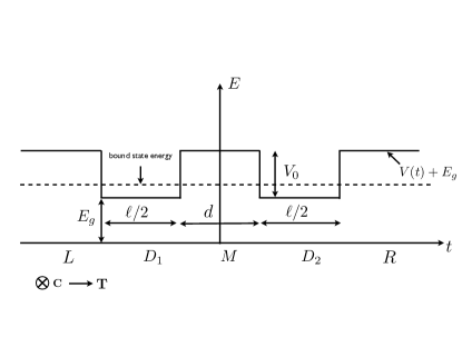
Figure 2: Energy diagram of a symmetrical CNT-DQD with electrostatic gates inducing a potential $V(t)$ along the nanotube axis; the origin is chosen in the center of the double dot, and the energy reference point is chosen in the middle of the gap. Two dots $D_{1}$ and $D_{2}$ of length $\ell/2$ each are tunnel coupled via a middle barrier $M$ of width $d$. The bound state energy $E$ (shown by dashed line) obeys the criterion $E_{g}<E<V_{0}+E_{g}$.

In this section we outline a model of a CNT-DQD motivated by the experimental setup in Ref. Churchill, . The underlying geometry is sketched in Fig. 2. The potential along the nanotube is controlled by top gates. For simplicity, we choose a double-well potential to model the double dot, similarly to Refs. Bulaev, and Wunsch, ,

$$V(t)=\left\{\begin{array}[]{rcl}V_{0},&&|t|<d/2,\,\,|t|>(d+\ell)/2\\ 0,&&d/2\leq|t|<(d+\ell)/2\end{array}\right.$$ (18)

and solve the eigenvalue problem for the Hamiltonian

$$H(t)=\hbar v(\tau k_{c}\sigma_{1}+k_{t}\sigma_{2})+\left(\Delta_{0}\tau+{1\over 2}g\mu_{B}B\right)s+V(t),$$ (19)

with $k_{c}$ of Eq. (12). The potential $V(t)$ is considered as step-like on the scale of the Fermi wavelength, $2\pi/k_{t}$, but smooth on the scale of the inverse Brillouin momentum, $2\pi/|K^{\tau}|$. Therefore, it does not induce essential ${\bf K}^{+}{\bf K}^{-}$-scattering. This is indeed relevant for an electrostatically confined dot. We calculate the single electron wavefunction for the symmetric geometry shown in Fig. 2 for equal confining potentials of the left and right wells, $V_{1}=V_{2}=V_{0}$. The two QDs are connected by a barrier of width $d$. The generalization to an asymmetric geometry is straightforward and will result in a larger electron wavenumber for the deeper well. The total energy of the system, $E=E_{1}+E_{2}$, will be considered fixed. In Eq. (19), the term in the second parentheses produces an $(s,\tau)$ dependent level shift but does not influence the wave functions. For the electronic wavefunction $\psi^{\tau}(t)$, defined in different intervals, see Fig. 2, we use the ansatz

$$\psi^{\tau}_{L}(t) = Ae^{q_{t}t}\left(\begin{array}[]{cc}z^{\tau}_{k_{c},-iq_{t}}\\ 1\end{array}\right),$$ (22)

$$\psi^{\tau}_{D_{1}}(t) = Be^{ik_{t}t}\left(\begin{array}[]{cc}z^{\tau}_{k_{c},k_{t}}\\ 1\end{array}\right)+Ce^{-ik_{t}t}\left(\begin{array}[]{cc}z^{\tau}_{k_{c},-k_{t}}\\ 1\end{array}\right),$$ (27)

$$\psi^{\tau}_{M}(t) = De^{-q_{t}t}\left(\begin{array}[]{cc}z^{\tau}_{k_{c},iq_{t}}\\ 1\end{array}\right)+Ee^{q_{t}t}\left(\begin{array}[]{cc}z^{\tau}_{k_{c},-iq_{t}}\\ 1\end{array}\right),$$ (32)

$$\psi^{\tau}_{D_{2}}(t) = Fe^{ik_{t}t}\left(\begin{array}[]{cc}z^{\tau}_{k_{c},k_{t}}\\ 1\end{array}\right)+Ge^{-ik_{t}t}\left(\begin{array}[]{cc}z^{\tau}_{k_{c},-k_{t}}\\ 1\end{array}\right),$$ (37)

$$\psi^{\tau}_{R}(t) = He^{-q_{t}t}\left(\begin{array}[]{cc}z^{\tau}_{k_{c},iq_{t}}\\ 1\end{array}\right),$$ (40)

with $z^{\tau}$ factors defined for electrons and holes, respectively, according to Eq. (4). In the gate regions, the electron wavenumber is determined as

$$q_{t}=\sqrt{k_{c}^{2}-(E_{k_{c},k_{t}}-V_{0})^{2}/(\hbar v)^{2}}.$$ (42)

Since the Hamiltonian $H(t)$ of Eq. (19) remains invariant under complex conjugation accompanied by $k_{t}\rightarrow-k_{t}$, the wavefunctions of Eq. (LABEL:ansatzwave) can be chosen in such a way that $C=B^{*}$, $G=F^{*}$, and $A$, $D$, $E$, and $H$ are real.

Energy levels are found from a transcendental equation that follows from the continuity of the wavefunction $\psi^{\tau}(t)$ at all potential steps. Since $v_{t}=\partial H/\partial p_{t}=v\sigma_{2}$, this equation maintains the current continuity. All coefficients in Eq. (LABEL:ansatzwave) can be calculated from the boundary conditions and the normalization condition. For $0<V_{0}<2E_{g}$, at least one electron bound state exists in each of the dots, and we will restrict ourselves only with the ground state (GS) mode. In a double dot, it splits into two, bonding and antibonding, with energies $E_{b}$ and $E_{ab}$, respectively .

The energy spectrum of the bonding mode of the Hamiltonian $H(t)$ of Eq. (19) is plotted in Fig. 3(a) as a function of an axial magnetic field in the absence of SO coupling. Having in mind narrow gap nanotubes,Churchill we choose $k_{g}=-0.045\mbox{ nm}^{-1}$, which produces a gap of about $2E_{g}\approx 46$ meV that is eight times less than estimated according to Eq. (6) for $\nu=1$ semiconducting tubes with $R\sim 1\mbox{ nm}$. In the absence of SO coupling, the $B=0$ state is four-fold degenerate in $s$ and $\tau$, and its splitting by magnetic field $B$ is shown in Fig. 3(a). Fig. 3(b) demonstrates the splitting of the $B=0$ state by SO coupling into a doublet of two pairs of Kramers conjugate states, ($|K^{+}_{\uparrow}\rangle,|K^{-}_{\downarrow}\rangle$) and $(|K^{+}_{\downarrow}\rangle,|K^{-}_{\uparrow}\rangle)$. The zero-field splitting is $\Delta_{SO}^{e}\approx 0.37$ meV, according to the data of Ref. Kuemmeth, and in a reasonable agreement with the data of Ref. Churchill, . The $B$-dependence in Fig. 3(b) reproduces correctly the patterns observed experimentally in Refs. Kuemmeth, and Churchill, . The effective $g$-factor, $\partial\Delta E/\partial(\mu_{B}B_{||})$, of the upper (lower) doublet is smaller (larger) due to the coupling of real spin to isospin.

The upper branch crossing in Fig. 3(b) persists for ${\bf B}\parallel{\bf T}$, but turns into an avoided crossing when $\bf B$ acquires a perpendicular component.Churchill Spin relaxation near this crossing was investigated in Refs. Churchill, , Bulaev, , and Rudner, . The lower branch crossing, at much lesser fields $B$, turns into an avoided crossing by ${\bf K}^{+}{\bf K}^{-}$ scattering with large momentum transfer, $\Delta_{K^{+}K^{-}}$. In high quality nanotubes of Refs. Kuemmeth, and Churchill, , where both $\Delta_{SO}$ and $\Delta_{K^{+}K^{-}}$ were observed experimentally, $\Delta_{K^{+}K^{-}}$ was nearly one order of magnitude less than $\Delta_{SO}$; in what follows, we disregard $\Delta_{K^{+}K^{-}}$. Its origin is not well understood for now, and it is usually attributed to electron scattering by defects.Bulaev

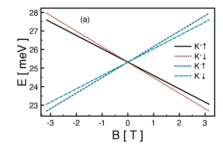
Figure 3: (color online) Magnetic field dependence of the energy of the bonding mode of a single-electron DQD for $k_{g}=-0.045$ nm^-1 and $\ell=200$ nm, $d=120$ nm, $V_{0}=3.95$ meV. The ground state energy $E_{GS}$ is close to the gap edge, $E_{GS}-E_{g}=1.4$ meV. (a) SO coupling is absent, $\Delta_{SO}=0$. At $B=0$, the spectrum is four-fold degenerate. (b) SO split energy spectrum. The zero field splitting between Kramers doublets is $\Delta_{SO}=0.37$ meV (with $\Delta_{1}=-0.15$ meV and $\Delta_{0}=0.04$ meV), see text for details.

Next, we discuss the longitudinal part of the wavefunction $\psi^{\tau}(t)$ and begin with exact symmetries of wavefunctions. Substituting Eq. (12) into Eq. (19), one arrives at a Hamiltonian $H_{\tau,s,B}(t)$. It includes the parameters $(\tau,s,B)$ only as time-inversion symmetric products $\tau B$ and $\tau s$. Therefore, $H_{-\tau,-s,-B}(t)=H_{\tau,s,B}(t)$, and wavefunctions can be chosen in such a way that they possess the same symmetry

$$\psi^{A(B)}_{\tau,s,B}(t)=\psi^{A(B)}_{-\tau,-s,-B}(t),$$ (43)

for an arbitrary potential $V(t)$. The superscripts $A$ and $B$ indicate sublattice indices. For symmetric dots, $V(t)=V(-t)$, one more relation holds. Performing a canonical transformation of $H_{\tau,s,B}(t)$ with a matrix $\sigma_{1}$, one notices that the sign change of the term $k_{t}\sigma_{2}$ can be compensated by a $t\rightarrow-t$ transformation. Because the $\sigma_{1}$ transformation transposes sublattices, $\sigma_{1}\left(\begin{array}[]{c}\psi^{A}\\ \psi^{B}\end{array}\right)=\left(\begin{array}[]{c}\psi^{B}\\ \psi^{A}\end{array}\right)$, wavefunctions obey the further relations

$$\psi^{A(B)}_{\tau,s,B}(t)=\pm\psi^{B(A)}_{\tau,s,B}(-t).$$ (44)

Here and in what follows we choose wavefunctions in such a way that they are real in the classically forbidden regions, which is always possible because the $z$-factors of Eq. (4) are real there. We note that in the left and right hand sides of Eq. (44) the $A(B)$ sublattices are interchanged. This reflects an absence of the microscopic $t\rightarrow-t$ symmetry in chiral nanotubes. Therefore, it is also absent in “symmetric” DQDs despite the macroscopic symmetry of the confining potential. Manifestations of this asymmetry are discussed next. Numerical data for the wavefunctions are presented in Fig. 4. Due to the exact symmetries of Eqs. (43) and (44), it is enough to display only a few curves demonstrating the basic regularities. Real parts of the wavefunctions of the bonding and antibonding modes are shown in Fig. 4(a). Their different behavior inside the tunnel barrier is distinctly seen. Also, $A$ and $B$ components of wavefunctions are nearly symmetric and antisymmetric for the bonding and antibonding modes, respectively. Technically, the asymmetry arises due to the admixture of the valence band wavefunctions and is small because the GS binding energy, $E_{GS}-E_{g}\approx 1.4$ meV, is small compared to the gap, $E_{g}\approx 23$ meV (or, what is essentially the same, $k_{t},q_{t}\ll|k_{g}|$). This asymmetry increases with $(E_{GS}-E_{g})$ and can become of the order of unity for $|E_{GS}-E_{g}|\sim E_{g}$.Rudner The opposite signs of the functions $\psi^{A}(t)$ and $\psi^{B}(t)$ originate from $k_{g}<0$. Fig. 4(b) displays small differences in the electron densities on both sublattices and their asymmetries that have the same origin as in Fig. 4(a).

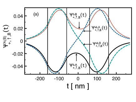
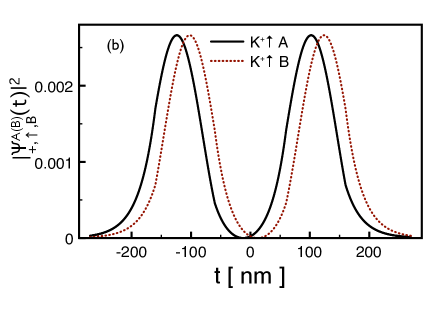
Figure 4: (color online) Single particle wavefunctions $\psi^{A(B)}_{+,\uparrow,B}(t)$ of a DQD for the same parameter values as in Fig. 3 and $B=1$ T. Vertical lines sketch edges of both dots. (a) Real parts of $\psi^{A(B)}_{+,\uparrow,B}(t)$ on both $A(B)$ sublattices are shown for bonding and antibonding modes, denoted by the superscripts $a$ and $ab$, respectively. At $t=0$ the former modes retain a considerable amplitude, whereas the latter vanish at the origin. Note that at each point the $A$ and $B$ components have nearly the same absolute values but opposite signs. (b) Electron density distribution in the bonding state; a non-vanishing density at $t=0$ is visible as well as a $t\rightarrow-t$ asymmetry and difference between $A$ and $B$ densities.

Within the GS approximation, the appearance of bonding (lower) and antibonding (upper) tunnel components, denoted as $\psi^{b}$ and $\psi^{ab}$, respectively, see Fig. 4, motivates a treatment of the orbital degrees of freedom of a DQD in terms of an effective two level system. Its eigenstates may be obtained by hybridization of the electron states localized in $D_{1}$ or $D_{2}$. Using the wavefunctions of Eq. (LABEL:ansatzwave) and notations of Eq. (44), we define the orbital basis states for certain spin and isospin (i.e., $|LK^{\tau}_{s}\rangle$ and $|RK^{\tau}_{s}\rangle$) in the left and right halfspaces, respectively, as

$$|LK^{\tau}_{s}\rangle = \frac{1}{\sqrt{2}}\left[\psi_{\tau,s,B}^{b}(t)+\psi_{\tau,s,B}^{ab}(t)\right],$$

$$|RK^{\tau}_{s}\rangle = \frac{1}{\sqrt{2}}\left[\psi_{\tau,s,B}^{b}(t)-\psi_{\tau,s,B}^{ab}(t)\right],$$ (45)

with associated energies $E_{\tau s}(B)$; these energies include also the second term of Eq. (19). Each of these functions is a two-spinor in sublattice space defined by its $A(B)$ components, and $K^{\tau}_{s}$ indicates that they should be chosen with $k_{c}$ of Eq. (12) calculated for proper values of $(\tau,s)$. This parametric dependence of the orbital functions on $s$ and $\tau$ stems from SO coupling and will be essential for the classification of quantum states, see Sec. III.1 below.

The connection between these basis states via tunneling is naturally established by the overlap of the wavefunctions in the interval $|t|\leq d/2$. The resulting spin and isospin conserving Hamiltonian expressed in this basis is

$$H_{RL}=\left(\begin{array}[]{cc}E_{k_{c},k_{t}}^{\tau sR}-\varepsilon&\eta_{\tau,s}\\ \eta_{\tau,s}&E_{k_{c},k_{t}}^{\tau sL}+\varepsilon\end{array}\right),$$ (46)

where $E_{k_{c},k_{t}}^{\tau sL}=E_{k_{c},k_{t}}^{\tau sR}=\frac{1}{2}\left(E_{b}^{\tau s}+E_{ab}^{\tau s}\right)$ are the single particle energies and $\varepsilon$ is the detuning between the left and right dot. The connection between left and right halfspaces, established by tunneling, produces bonding and antibonding states of Eq. (19). The tunnel matrix element $\eta_{\tau,s}$ is related to their energy difference as

$$2\eta_{\tau,s}=E^{\tau s}_{b}-E^{\tau s}_{ab}.$$ (47)

Equivalently, the tunneling part $H_{T}$ of the Hamiltonian of Eq. (46) can be rewritten in terms of the orbital functions $|L(R)K^{\tau}_{s}\rangle$ in a form that is more convenient for further calculations

$$H_{T}=\sum_{\tau=\pm,s=\uparrow,\downarrow}\eta_{\tau,s}\left[|LK^{\tau}_{s}\rangle^{A(B)}\langle RK^{\tau}_{s}|^{A(B)}+h.c.\right].$$ (48)

The matrix elements $\eta_{\tau,s}$ are plotted in Fig. 5 as a function of $B$ for the parameter values used in Fig. 3(b). The zero field difference in the tunneling matrix elements stems from the $\Delta_{1}$ term in Eq. (12). They are nearly linear functions of $B$ in the whole region of magnetic field and their absolute values are larger for the lower Kramers doublet. This fact is also reflected in the following inequality for the wavenumbers in the classically forbidden regions, $q_{t}(K^{+}_{\uparrow})>q_{t}(K^{+}_{\downarrow})$, cf. Eq. (42), that holds for our set of parameter values. Since the Hamiltonian $H(t)$ of Eq. (19) is symmetric with respect to time inversion, $\eta_{\tau,s}(B)=\eta_{-\tau,-s}(-B).$

We note that a change of the sign $k_{g}$, to $k_{g}>0$, with the values of $\Delta_{0}$ and $\Delta_{1}$ recalculated properly to keep the right slopes in Fig. 3(b) ($\Delta_{0}=-0.04$ meV and $\Delta_{1}=-0.15$ meV), keeps Fig. 5 practically unchanged with the upper doublet having a lesser tunneling rate (absolute value of $\eta$), since the sign of $\Delta_{1}$ remains intact. Therefore, these data do not constrain the sign of $k_{g}$ either. Such a behavior of the tunneling rates seems counterintuitive, but it stems from the fact that the rates are controlled by the sign of $\Delta_{1}$ while the nature of the upper and lower Kramers doublets is insensitive to it.

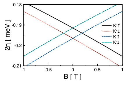
Figure 5: (color online) Tunneling matrix elements $\eta_{\tau,s}(B)$ plotted versus magnetic field. Their absolute values are larger for the lower Kramers doublet $(K^{+}_{\downarrow},K^{-}_{\uparrow})$. For $B=0$, they depend on spin and isospin through the product $s\tau$. The zero field difference in the tunneling rate originates from $\Delta_{1}\neq 0$ and vanishes for $\Delta_{1}\to 0$. Parameter values are the same as in Fig. 3(b).

Fig. 6 shows the effect of detuning $\varepsilon$ on the energy spectrum of the Hamiltonian Eq. (46). In our calculations, we have consistently used the $\tau,s,$ and $B$ dependencies of the matrix elements $\eta_{\tau,s}(B)$ derived from Eq. (47). Cyan (dash-dotted) and red (dotted) lines in Fig. 6(a) correspond to the upper and lower Kramers doublets. In the absence of a magnetic field all states are two-fold Kramers degenerate. For $B\neq 0$ this degeneracy is lifted; the spectrum for $B=1\mbox{ T}$ is shown in Fig. 6(b). Energies corresponding to various bonding (antibonding) and spin (isospin) states are shown in the same colors and line patterns as in Fig. 3. The spectrum splitting in a magnetic field originates from the Aharonov-Bohm flux $\Phi_{AB}$ of Eq. (12) (that can be ascribed to an orbital magnetic moment $\mu_{\rm orb}$) and the Zeeman spin splitting described by the next-to-last term in Eq. (19). Because $\mu_{\rm orb}\sim 10\mu_{B}$,Minot ; Kuemmeth ; Churchill the first contribution dominates and both spin components of the $K^{-}$ state move up in energy with increasing $B$. The asymmetry in the level splittings inside the upper and lower quadruplets in the large $B$ region originates from the interference of the SO and Zeeman splittings in each of the single dots.Kuemmeth ; Churchill

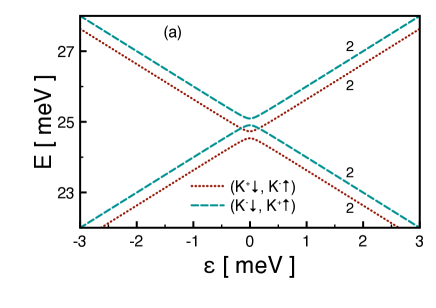
Figure 6: (color online) Detuning dependence of the energy spectrum of a single-electron DQD. Tunnel matrix elements $\eta_{\tau,s}$ from Fig. 5 are used for the respective states, other parameters as in Fig. 3. (a) Both Kramers doublets (identified by color) split into bonding and antibonding modes. The numbers denote energy level multiplicity. (b) Level splitting by magnetic field $B=1$ T. Because of the dominating effect of the Aharonov-Bohm flux, $K^{-}$ components with both $s=\uparrow,\downarrow$ move upwards. The magnitudes of the avoided crossings at $\varepsilon=0$, seen both in (a) and (b), are controlled by $\eta_{\tau,s}$.

III Two electron regime

Charge states in DQD systems are usually described in terms of stability diagrams.vanderWiel ; Hanson ; Churchill Either from Coulomb blockade peaks in transport measurements or from charge sensing probes, the number of electrons $n_{L}$ and $n_{R}$ in the respective dot is monitored. In the following we consider the two electron regime. There are two possible physical realizations of it depending on the adjustment of the confinement potentials for the left and right dot and the tunneling barrier between them. First, two electrons are confined to a single dot, here the right dot, denoted the $(02)$ configuration. Otherwise, both electrons are confined in different dots, which is referred to as the $(11)$ configuration. Experimentally, it is possible to drive the DQD between the two regimes by applied gate voltages if both dots are connected by a tunneling barrier.

III.1 $(02)$ Configuration

For a two-electron system without SO coupling, a classification of two-electron states in terms of singlet and triplet states in real spin is exact due to the Pauli principle.QuantMech Here, when constructing two-electron states, we use the Hilbert space spanned by the lowest energy orbitals in each dot. Because the spin and orbital degrees of freedom are coupled, a classification in terms of spin singlet and triplets is no longer applicable. Technically, this means that a full basis of two-particles states in the space of functions respecting the Pauli exclusion principle cannot be constructed in terms of products of spin singlets (triplets) and linear combinations of products of the orbital functions $|L(R)K^{\tau}_{s}\rangle$ of Eq. (45). Spin singlets and triplets become coupled, and using such generalized basis states we arrive at the results that are quite general and, in particular, can be applied in the vicinity of the point where $k_{c}$ vanishes due to the cancellation of different terms in Eq. (12); the latter regime has been reported recently for a single dot.Jhang However, the regime where the gap between the conduction and valence bands closes completely (see Ref. Jhang, ) is not addressed here, since it does not allow for electrostatic confinement of electrons or holes.

With two electrons bound to the right dot, there are six linearly independent antisymmetric basis functions. Two of them, with both spins either up or down, can be considered as components $T_{\pm 1}$ of a spin triplet. They are

$$|\Phi^{02}_{s}\rangle={{1}\over{\sqrt{2}}}\left(|RK^{+}_{s}s\rangle_{1}|RK^{-}_{s}s\rangle_{2}-1\rightleftharpoons 2\right),$$ (49)

with $|\Phi^{02}_{1}\rangle$ for $s=\uparrow$ and $|\Phi^{02}_{2}\rangle$ for $s=\downarrow$, and the symbol $1\rightleftharpoons 2$ indicates electron transposition. Here $|RK^{\pm}_{s}s\rangle$ are products of orbital functions $|RK^{\pm}_{s}\rangle$ and their spin counterparts $|s\rangle$.

Four different functions, all with opposite spins, are spin-isospin coupled. Within the first pair of states, both electrons reside in the same $K^{\tau}$ point, but in such a way that in the $B=0$ limit one of the electrons belongs to the upper and the second to the lower Kramers doublet of Fig. 3

$$|\Phi^{02}_{\tau}\rangle={{1}\over{\sqrt{2}}}\left(|RK^{\tau}_{\uparrow}\uparrow\rangle_{1}|RK^{\tau}_{\downarrow}\downarrow\rangle_{2}-1\rightleftharpoons 2\right),$$ (50)

with $|\Phi^{02}_{3}\rangle$ for $\tau=+$ and $|\Phi^{02}_{4}\rangle$ for $\tau=-$. In the second pair of states, for $B=0$, both electrons populate the upper and lower Kramers doublets of Fig. 3

$$|\Phi^{02}_{u}\rangle = {{1}\over{\sqrt{2}}}\left(|RK^{+}_{\uparrow}\uparrow\rangle_{1}|RK^{-}_{\downarrow}\downarrow\rangle_{2}-1\rightleftharpoons 2\right),$$

$$|\Phi_{l}^{02}\rangle = {{1}\over{\sqrt{2}}}\left(|RK^{-}_{\uparrow}\uparrow\rangle_{1}|RK^{+}_{\downarrow}\downarrow\rangle_{2}-1\rightleftharpoons 2\right).$$ (51)

We designate them as $|\Phi^{02}_{5}\rangle$ and $|\Phi^{02}_{6}\rangle$, respectively.

Equations (49)-(51) demonstrate the profound effect of SO coupling on the symmetry of the $(02)$ multiplets: Since spin and isospin are coupled, those states cannot be represented in terms of spin singlet and triplets. The energy spectrum is SO split. In the absence of a magnetic field, $B=0$, the state $\mid\Phi_{5}\rangle$ ($\mid\Phi_{6}\rangle$) has the highest (lowest) energy because both electrons populate the upper (lower) Kramers doublet, while the four other states are mutually degenerate because one of the electrons populates the upper and the second the lower state.

III.2 Coulomb Matrix Elements

We choose the Coulomb potential as

$$V_{C}=\frac{e^{2}}{4\pi\epsilon_{0}\kappa}\frac{1}{\sqrt{a_{z}^{2}+(t_{1}-t_{2})^{2}+(2R)^{2}\sin^{2}[(\varphi_{1}-\varphi_{2})/2]}},$$ (52)

with $\kappa$ as an effective dielectric constant. The cut-off term $a^{2}_{z}\approx(2a_{B})^{2}$, with $a_{B}$ for the Bohr radius, accounts for the size of $2p_{z}$ functions.Reinhold Such a cut-off is convenient in numerical calculations but has no essential effect on the final results because Coulomb matrix elements converge in two dimensions at small electron separations. In what follows, we calculate matrix elements of $V_{C}$ for both the $(02)$ and $(11)$ configurations. Similarly, while taking into account consistently the SO corrections to functions $|K^{\tau}_{s}\rangle$ in both dots, we keep only spin-diagonal terms when calculating the Coulomb matrix elements and therefore exclude spin nonconserving processes. This approximation is motivated by our focus on dots with small radius $R$ and narrow gap $E_{g}\approx\hbar vk_{c}$; indeed, the diagonal SO corrections are large in inverse $k_{c}$ while nondiagonal SO terms are suppressed for small $R$ by strong orbital quantization in the circular direction.AndoSO In exchange matrix elements for the $(02)$ configuration, a selection rule for $\tau$ appears from the fact that $V_{C}$ depends on $(\varphi_{1},\varphi_{2})$ only through their difference. Upon using notations $|\tau s\rangle$ for kets including products of the orbital functions $|K^{\tau}_{s}\rangle$ and the corresponding spin functions $|s\rangle$, we take advantage of Eq. (13) and find

$$\langle{\tau_{1}}{s_{1}}(1),{\tau_{2}}{s_{2}}(2)|V_{C}(1,2)|{\tau_{3}}{s_{3}}(2),{\tau_{4}}{s_{4}}(1)\rangle$$

$$\propto \int_{0}^{2\pi}d\varphi\exp{[-i(M+n_{2}/2)(\tau_{1}+\tau_{2}-\tau_{3}-\tau_{4})\varphi]},$$

where $\varphi=(\varphi_{1}+\varphi_{2})/2$. Expressing $M$ in terms of the chiral indices $(n_{1},n_{2})$ results in $(M+n_{2}/2)=n_{1}/3+n_{2}/6-\nu/3$. Hence, inside the irreducible wedge of the Bravais lattice where $0\leq\theta<\pi/6$ and $n_{1},n_{2}\geq 0$, it is always true that $(M+n_{2}/2)\neq 0$, and therefore

$$\tau_{1}+\tau_{2}=\tau_{3}+\tau_{4}.$$ (54)

Comparing Eq. (54) with the spin selection rule $s_{1}=s_{4}$, $s_{2}=s_{3}$ (in the leading approximation in SO) underscores a fundamental difference between the spin and isospin, which is an orbital quantum number.

Under these assumptions, $V_{C}$ of Eq. (52) is represented in the basis of $\Phi^{02}$-functions of Eqs. (49)-(51) as

$${\hat{V}}_{C}^{02}=\left(\begin{array}[]{cccccc}U_{02}^{\uparrow}-J^{\uparrow}_{02}&0&0&0&0&0\\ 0&U^{\downarrow}_{02}-J_{02}^{\downarrow}&0&0&0&0\\ 0&0&U_{02}^{+}&0&0&0\\ 0&0&0&U_{02}^{-}&0&0\\ 0&0&0&0&U_{02}^{u}&J_{02}\\ 0&0&0&0&J_{02}&U_{02}^{\ell}\end{array}\right).$$ (55)

It includes six Coulomb matrix elements $U_{02}$ and three exchange matrix elements $J_{02}$. The latter ones include terms that are nondiagonal in $\tau$ but obey the selection rule of Eq. (54); one can show that the nondiagonal matrix elements $J_{02}$ are real. The absence of isospin indices in $U_{02}^{\sigma}$ and $J_{02}^{\sigma}$ indicates that electrons belong to different valleys. Similarly, the absence of spin indices in $U_{02}^{\tau}$ indicates that electrons possess opposite spins.

All Coulomb terms $U_{02}$ have a universal form in the framework of our model and do not depend on the chirality of the nanotube. As distinct from them, exchange integrals $J_{02}$ depend on chirality and, what is even more important, include products of orbital functions $|RK^{\tau}_{s}\rangle$ with different values of $\tau$. Therefore, they require large momentum transfer of $4\pi/3a$, which is accompanied by fast oscillating factors in the integrands. The calculation of such integrals cannot be performed using envelope functions of Eq. (3) and requires including microscopic Bloch functions of graphene and short range interaction potentials. This is outside the framework of our model, and since such integrals are small, we disregard them in what follows.

Figure 7: (color online) Magnetic field dependence of the Coulomb matrix elements $U_{02}$ in a single QD with dielectric constant $\kappa=1$. Parameters are the same as in Fig. 3(b). The $B$ dependence is strong for isospin polarized states $|\Phi^{02}_{3}\rangle$ and $|\Phi^{02}_{4}\rangle$, with the opposite signs of the slope for $\tau=\pm$. For isospin unpolarized states the $B$-dependences are weak. The energies $U_{02}^{\uparrow}$ and $U_{02}^{\downarrow}$ nearly coincide. For $B=0$, the largest difference in $U_{02}$ energies is achieved for the states with both electrons belonging to the lower or upper Kramers doublet. The matrix elements $U_{02}$ strongly influence the position of the $(11)$-$(02)$ degeneracy point in Figs. 9 and 10 below.

The six different Coulomb integrals $U_{02}$ and their magnetic field dependence are shown in Fig. 7 for $\kappa=1$. As distinct from the single electron levels of Fig. 3, where the $B$ dependence originated from the orbital and spin magnetic moments, the $B$ dependence of $U_{02}$ integrals is determined by the $B$ dependence of the circumferencial wavenumber $k_{c}$ of Eq. (12) only. Remarkably, this dependence is much stronger for isospin polarized states $\mid\Phi^{02}_{3}\rangle$ and $\mid\Phi^{02}_{4}\rangle$ than for the other four states; for the latter ones, the $B$-dependencies are nearly identical. We attribute this behavior to the competition of the two largest terms in $k_{c}$, namely the first and second one of Eq. (12), which therefore does not rely on SO coupling. In $\mid\Phi^{02}_{3}\rangle$ and $\mid\Phi^{02}_{4}\rangle$ both electrons have the same isospin $\tau$, hence the same $B$-dependences of $k_{c}$ add, while in all other functions the electrons have opposite signs of $\tau$ and the $B$-dependences subtract. We note that in the absence of SO coupling, Coulomb integrals for $\mid\Phi^{02}_{1}\rangle,\mid\Phi^{02}_{2}\rangle,\mid\Phi^{02}_{5}\rangle,\mid\Phi^{02}_{6}\rangle$ coincide for all magnetic fields. For nanotubes coated by an insulator, as in experiments by Churchill et al.Churchill ; Churchill2 , the Coulomb repulsion is reduced by a factor of $\kappa\approx 10$. It should be noted that the metallic gates used in the experimental setups also strongly screen the Coulomb interaction, and in particular they cut-off the long range part of it. Therefore, the absolute numbers for the Coulomb matrix element that we find here are subject to changes depending on the experimental details, however the general trends based on the symmetry of the two-particle wavefunctions remains.

III.3 Energy spectrum

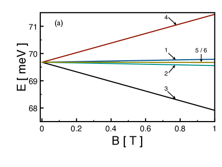
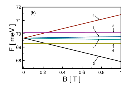
Figure 8: (color online) Magnetic field dependence of the energy spectrum of a two-electron single QD. Coulomb interaction is screened by $\kappa=10$; other parameters are the same as in Fig. 3. (a) Without SO coupling the spectrum is six-fold degenerate at $B=0$, and its $B$ dependence originates mostly from the coupling of the orbital and spin magnetic moments to the field. Wavefunctions can be represented as spin singlets–isospin triplets and spin triplets–isospin singlets. (b) With SO coupling the spectrum is split at $B=0$. The level crossing at finite $B$ results in a ground state change from two electrons populating the lower Kramers doublet to two isospin polarized electrons. Numbers with arrows denote the energy that corresponds to a particular state among $\mid\Phi^{02}_{1,\dots,6}\rangle$.

The results for the magnetic field dependence of the energy levels of a two-electron QD are shown in Fig. 8. We have diagonalized the two particle Hamiltonian for a single QD, cf. Ref. Bulaev, , in the presence of SO coupling as well as a screened Coulomb interaction, $\kappa=10$. QD parameters are chosen as in Sec. II.2. The $B$ dependence of the Coulomb interaction terms $U_{02}$ was taken into account consistently. The comparison of panels (a) and (b) demonstrates the effect of SO coupling. In the absence of SO coupling, Fig. 8(a), the hexaplet remains unsplit at $B=0$ because $J_{02}$ exchange integrals are disregarded. For $\Delta_{SO}=0$, a classification of these degenerate states in terms of a spin singlet (isospin triplet) and a spin triplet (isospin singlet) is appropriate. The $B$ dependence of the isospin polarized states $|\Phi^{02}_{3}\rangle,|\Phi^{02}_{4}\rangle$ and spin polarized states $|\Phi^{02}_{1}\rangle,|\Phi^{02}_{2}\rangle$ originates mostly from their orbital and spin magnetic moments, respectively. In the whole region of magnetic fields, the ground state is isospin polarized with both electrons in the $\tau=1$ state having opposite spins. SO coupling splits the hexaplet at $B=0$, see Fig. 8(b), with both electrons populating the lower Kramers doublet in the lowest state $|\Phi^{02}_{6}\rangle$. The level crossing at $B\approx 0.3\mbox{ T}$ results in a change of the ground state. This transition might also be seen in the two electron spectrum of Ref. Kuemmeth, . At larger fields, the ground state becomes well separated from all higher states.

Although we do not calculate electron attraction due to their coupling to phonons, we note that an estimate shows that it might become comparable to a screened Coulomb repulsion for $\kappa\gtrsim 10$. A more detailed investigation of this contribution is needed.

IV Two particle spectrum as a function of detuning

In recent experiments,Churchill the dephasing time $T_{2}^{*}$ of a two particle state was obtained by the following measurement cycle. First the system is prepared in the $(02)$ configuration whose ground state is non-degenerate for a CNT-DQD, Fig. 8(b). The doubly occupied right dot might be considered as a double dot in a strongly detuned state where the detuning energy $\varepsilon$ compensates the strong Coulomb repulsion; hence, it is energetically favorable for two electrons to populate the same dot. When decreasing $\varepsilon$, the Coulomb repulsion and interdot tunneling allow pushing one of the electrons to the left dot, and the system is transferred into the $(11)$ configuration. This produces an additional degree of freedom, manifesting itself in a quantum well index $L(R)$, and allowing for 16 states in the $(11)$ configuration, as compared to 6 states in the $(02)$ configuration. The whole space includes $22$ basis states. The transfer of the system from the six-fold $(02)$ space to sixteen-fold $(11)$ space is followed by dephasing due to different mechanisms, including hyperfine interactions and isospin scattering. When $\varepsilon$ is increased again, after a certain separation time $\tau_{S}$, the system is prevented from coming back because not all states from $(11)$ are connected by tunneling to the states in $(02)$. This generalized Pauli blockade arises from the selection rules both in spin and isospin. The probability of finding both electrons again in the right dot depends on $\tau_{S}$, and measuring the return probability as a function of $\tau_{S}$ is used to extract $T_{2}^{*}$, as has been done for CNT-DQDs with $T_{2}^{*}=3.2$ ns.Churchill Therefore, $T_{2}^{*}$ should strongly depend on the coupling between the energy levels of the $(02)$ and $(11)$ subsystems that will be investigated below.

IV.1 $(11)$ configuration

In this section we construct a basis of the two-particle Hilbert space of the $(11)$ configuration starting from the $(02)$ configuration basis and using the corresponding single-particle wavefunctions of Eq. (45). Consider, e.g., the state of Eq. (49) with spin polarized functions $\mid\Phi_{s}^{02}\rangle$. There are two possibilities, either the first or the second electron can occupy the right dot,

$$\mid\Phi_{Is}^{11}\rangle = \frac{1}{\sqrt{2}}\left(\mid RK^{+}_{s}s\rangle_{1}\mid LK^{-}_{s}s\rangle_{2}-1\rightleftharpoons 2\right),$$

$$\mid\Phi_{\tilde{Is}}^{11}\rangle = \frac{1}{\sqrt{2}}\left(\mid LK^{+}_{s}s\rangle_{1}\mid RK^{-}_{s}s\rangle_{2}-1\rightleftharpoons 2\right).$$ (56)

This procedure, when applied to the states $\mid\Phi_{1,\dots,6}^{(02)}\rangle$ of Eqs. (49), (50) and (51), results in twelve states of the $(11)$ configuration. From those twelve states we construct combinations that are symmetric and antisymmetric in $L/R$ space. For example, from Eq. (56) we find for $s=\uparrow$

$$\mid\Phi_{1\pm}^{11}\rangle\equiv\frac{1}{\sqrt{2}}\left(\mid\Phi_{I\uparrow}^{11}\rangle\pm\mid\Phi_{\tilde{I\uparrow}}^{11}\rangle\right),$$ (57)

We denote by $\mid\Phi^{11}_{1+,\dots,6+}\rangle$ and $\mid\Phi^{11}_{1-,\dots,6-}\rangle$, respectively, the symmetric and antisymmetric superpositions in $L/R$ space. In addition, in the $(11)$ configuration there are four states polarized in both spin and isospin

$$\mid\Phi_{i}^{11}\rangle=\frac{1}{\sqrt{2}}\left(\mid LK_{s}^{\tau}s\rangle_{1}\mid RK_{s}^{\tau}s\rangle_{2}-1\leftrightharpoons 2\right).$$ (58)

All of them are antisymmetric; similar combinations in (02) are forbidden by the Pauli exclusion principle. We use the convention $i=13$ for $\tau=+,s=\uparrow$, $i=14$ for $\tau=+,s=\downarrow$, $i=15$ for $\tau=-,s=\uparrow$, and $i=16$ for $\tau=-,s=\downarrow$.

IV.2 Coulomb and tunneling matrix elements

We need to calculate a $16\times 16$ matrix of the Coulomb interaction in the $(11)$ configuration that is similar to Eq. (55), as well as one- and two-particle matrix elements that connect the $(02)$- and $(11)$-subspaces.

In the $(11)$ subspace, the matrix of direct Coulomb terms is diagonal and its matrix elements are equal for symmetric and antisymmetric combinations. Hence, we need to compute only six independent matrix elements for the twelve symmetric and antisymmetric states $|\Phi^{11}_{1\pm,\dots,6\pm}\rangle$. They are denoted as $U^{+}_{11},U^{-}_{11},U^{\uparrow}_{11},U^{\downarrow}_{11},U^{u}_{11},U^{l}_{11}$ according to the spins and isospins of the states involved. There are four additional Coulomb terms for the states $\mid\Phi^{11}_{13,14,15,16}\rangle$ that are both spin and isospin polarized. We denote their Coulomb matrix elements as $U_{11}^{\uparrow+},U_{11}^{\downarrow+},U_{11}^{\uparrow-},U_{11}^{\downarrow-}$. Since we have chosen the wavefunctions in such a way that they are real in the classically forbidden regions (see Sec. II.2) Coulomb matrix elements between the states $\mid\Phi_{1+,\dots,6+}\rangle$ and $\mid\Phi_{1-,\dots,6-}\rangle$ vanish. Furthermore, Coulomb integrals between $|\Phi_{1\pm,\dots,6\pm}\rangle$ and $|\Phi_{13,14,15,16}\rangle$ vanish because of the spin and isospin selection rules.

The strongest $B$-dependence occurs for the six matrix elements $(U_{11}^{+},U_{11}^{-},U_{11}^{\uparrow+},U_{11}^{\downarrow+},U_{11}^{\uparrow-},U_{11}^{\downarrow-})$ corresponding to the isospin polarized states (not shown here). Similarly to the $(02)$ configuration, we attribute this behavior to the $B$-dependence of $k_{c}$ of Eq. (12). However, comparing to the $(02)$ configuration (see Fig. 7) the slopes for $\mid\Phi^{02}_{3}\rangle$ and $\mid\Phi^{11}_{3\pm}\rangle$ have opposite signs. The same holds also for $\mid\Phi^{02}_{4}\rangle$ and $\mid\Phi^{11}_{4\pm}\rangle$.

In addition to the matrix of the direct Coulomb interaction discussed above, there are also exchange matrix elements. As distinct from the (02) configuration, in the $(11)$ configuration there exist a number of interdot exchange matrix elements that are not annihilated by the requirements of the spin conservation and the selection rule of Eq. (54). They include the overlapping densities between the left and right dot. Specifically, for $\mid\Phi_{1+}^{11}\rangle$,

$$J_{LR}^{\uparrow}=\langle LK^{-}_{\uparrow,2};RK^{+}_{\uparrow,1}\mid V_{C}\mid LK^{+}_{\uparrow,1};RK^{-}_{\uparrow,2}\rangle.$$ (59)

The generalization for other states is straightforward. We find that there are $10$ independent $J$-exchange matrix elements in the $(11)$ configuration. All of them are positive, and they are one order of magnitude smaller than the Coulomb terms for the parameters values chosen. In the (11) configuration, these exchange terms shift the energies of the antisymmetric states down and the symmetric states up.

Besides the $(11)$ terms in the Hamiltonian matrix calculated above, the cross-terms that provide a coupling between the $(11)$ and $(02)$ configurations are of critical importance. They originate both from the single-electron tunneling Hamiltonian $H_{T}$ and from the two-electron Coulomb Hamiltonian $V_{C}$ and connect all $|\Phi^{02}\rangle$ states with the first twelve $|\Phi^{11}\rangle$ states. The last four $|\Phi^{11}\rangle$ states of Eq. (58) cannot tunnel to the $(02)$ configuration by construction.

The first contribution is similar to Eq. (46), yielding twelve matrix elements

$$\langle\Phi_{s}^{02}\mid H_{T}\mid\Phi_{s\pm}^{11}\rangle = \frac{1}{\sqrt{2}}\left(\eta_{+,s}\pm\eta_{-,s}\right),$$

$$\langle\Phi_{\tau}^{02}\mid H_{T}\mid\Phi_{\tau\pm}^{11}\rangle = \frac{1}{\sqrt{2}}\left(\eta_{\tau,\uparrow}\pm\eta_{\tau,\downarrow}\right),$$

$$\langle\Phi_{u}^{02}\mid H_{T}\mid\Phi_{u\pm}^{11}\rangle = \frac{1}{\sqrt{2}}\left(\eta_{-,\downarrow}\pm\eta_{+,\uparrow}\right),$$

$$\langle\Phi_{l}^{02}\mid H_{T}\mid\Phi_{l\pm}^{11}\rangle = \frac{1}{\sqrt{2}}\left(\eta_{+,\downarrow}\pm\eta_{-,\uparrow}\right).$$ (60)

Here $H_{T}$ are sums of the tunnel Hamiltonians of Eq. (48) over both electrons, and $\eta_{\tau,s}$ are defined by Eq. (47). Note that $\pm$ signs in Eq. (60) correspond to symmetric and antisymmetric states in the $(11)$ configuration. At $B=0$, antisymmetric combinations $|\Phi^{11}_{5-,6-}\rangle$ are forbidden from tunneling to $(02)$ because of spin and isospin conservation and the relation $\eta_{\tau,s}(B)=\eta_{-\tau,-s}(-B)$ established in Sec. II.2. From Eq. (60) follows that antisymmetric combinations are not entirely forbidden from tunneling to the $(02)$ configuration because of the $(\tau,s)$ dependence of the tunneling matrix elements $\eta_{\tau,s}$. However, as one concludes from Fig. 5, this dependence is rather weak, only about 1%, and therefore transitions to $(02)$ states from antisymmetric $(11)$ states are strongly suppressed. It is in this sense that we discuss the left-right $(L/R)$ symmetry selection rules in what follows. Since they are approximate, the corresponding level crossings transform into narrow avoided crossings.

The second contribution originates from the Coulomb interaction and is also represented by 12 matrix elements

$$\langle\Phi_{s}^{02}\mid V_{C}\mid\Phi_{s\pm}^{11}\rangle = J_{02\leftrightarrow 11}^{s\pm},$$

$$\langle\Phi_{\tau}^{02}\mid V_{C}\mid\Phi_{\tau\pm}^{11}\rangle = J_{02\leftrightarrow 11}^{\tau\pm},$$

$$\langle\Phi_{u}^{02}\mid V_{C}\mid\Phi_{u\pm}^{11}\rangle = J_{02\leftrightarrow 11}^{u\pm},$$

$$\langle\Phi_{l}^{02}\mid V_{C}\mid\Phi_{l\pm}^{11}\rangle = J_{02\leftrightarrow 11}^{l\pm}.$$ (61)

All of them include overlap densities from the right and left dots. As an example, we present the exchange integral between the states $|\Phi_{1}^{02}\rangle$ and $|\Phi_{1\pm}^{11}\rangle$

$$J_{02\leftrightarrow 11}^{\uparrow\pm} = \frac{1}{\sqrt{2}}\left(\langle RK^{-}_{\uparrow;2}RK^{+}_{\uparrow;1}\mid V_{C}\mid RK^{+}_{\uparrow;1}LK^{-}_{\uparrow;2}\rangle\right.$$ (62)

$$\pm \left.\langle RK^{-}_{\uparrow;2}RK^{+}_{\uparrow;1}\mid V_{C}\mid LK^{+}_{\uparrow;1}RK^{-}_{\uparrow;2}\rangle\right).$$

Other exchange integrals of Eq. (61) have a similar structure and the $\pm$ signs refer to the symmetric and antisymmetric linear combinations in the $L/R$ degree of freedom for the $(11)$ configuration. The integrals of Eqs. (60) and (62) are subject to the same spin/isospin selection rules and contribute additively to all (avoided) crossings between the $(02)$ and $(11)$ states. Comparing Eqs. (59) and (62) one notices immediately that matrix elements including an odd (even) number of the wave functions of the left or the right dot have opposite (same) signs in the symmetric and antisymmetric states.

IV.3 Energy spectrum

For electron spin dynamics as well as for electron manipulation by gate voltages, the dependence of the energy levels on the detuning $\varepsilon$ between the two dots and the magnetic field $B$ is important. Especially, the position of the energy levels and the width of the avoided crossings that appear due to tunneling and exchange integrals might be observed in transport experiments on CNT-DQDs.

Fig. 9 presents the result of the two particle spectrum as a function of detuning at $B=0$. Other dot parameters are the same as in Fig. 3(b). In the lower right corner, the system is in the $(02)$ configuration and the ground state is given by $\mid\Phi^{02}_{6}\rangle$ with both electrons populating the lower Kramers doublet. The next group of states ($|\Phi^{02}_{s}\rangle$ with $s=\uparrow,\downarrow$ and $|\Phi^{02}_{\tau}\rangle$ with $\tau=\pm$) originates from the mixed populations of the two Kramers doublets. The splittings between their energies are controlled by the matrix elements $U_{02}^{\uparrow}$ and $U_{02}^{+}$, the first of which is small and the second vanishes at $B=0$, see Fig. 7. They are not resolved in Fig. 9.

When $\varepsilon$ decreases, the six $(02)$ states hybridize with their $|\Phi^{11}_{i+}\rangle$ counterparts and form lower and upper (bonding and antibonding) tunnel components, indicated by B and AB superscripts in the figure. The $(11)-(02)$ degeneracy point is located at $\varepsilon\approx U_{02}/2$. Here $U_{02}$ is a mean value of the integrals $U_{02}^{i}$ with $i=(\uparrow,\downarrow,+,-,u,l)$ defined in Sec. III.2 that differ only within 10% among each other. More accurate positions of the degeneracy points for specific transitions are $\varepsilon^{0}_{i}=[U_{02}^{i}-(U_{11}^{i}+J_{LR}^{i})]/2$ where $J_{LR}^{i}$ are exchange integrals defined by Eq. (38); $J_{LR}^{i}$ are only about a few percents of $U_{02}$. The widths of the tunnel doublets at $\varepsilon^{0}_{i}$ points can be found from Eqs. (60) and (62), for instance, for the up-spin state $|\Phi_{1}\rangle$ it equals $\sqrt{2}(\eta_{+\uparrow}+\eta_{-\uparrow})+2J^{\uparrow\pm}_{02\leftrightarrow 11}$. As seen in Fig. 9, the splitting between bonding and antibonding states becomes large in the vicinity of the $(11)$-$(02)$ degeneracy point and competes with the SO induced splitting.

We note that these equations do not involve the states $\mid\Phi^{11}_{13,14,15,16}\rangle$ since they are completely decoupled from all different states and pass through the whole region of the $(02)-(11)$ resonances without any avoided crossings.

Remarkable properties of the ground state deserve a special attention. In the absence of Coulomb interaction (or for very large $\kappa$), the ground state of the (11) configuration is controlled by tunneling and is a bonding state that is always symmetrical, see Fig. 4(a). However, because of the competition between tunneling, Eq. (60), and exchange, Eqs. (59) and (61), the ordering of levels can change. This reordering of levels is a real consequence of our calculations despite the large value of $\kappa=10$. The level of the symmetrical hybridized state of $|\Phi^{11}_{6+}\rangle$ and $|\Phi^{02}_{6}\rangle$ (designated as a bonding state $|\Phi^{B}_{6}\rangle$ in Fig. 9) crosses the level of the antisymmetric state $|\Phi^{11}_{6-}\rangle$ at the point highlighted by a circle in Fig. 9. While to the left from the circle these levels nearly merge in Fig. 9, they are well resolved in Fig. 11. Under such conditions, the ground states on the left and right from the $(11)$-$(02)$ resonance are not connected because of the highly unusual order in which the levels follow on the left, i.e., in the mostly (11) configuration. There the antisymmetric state lies below the symmetric one, as a consequence of the fact that the exchange integrals (see Sec. IV.2) prevail over the competing contribution of the tunneling matrix elements.

Besides the state $|\Phi^{11}_{6-}\rangle$ there are different (nearly) unconnected states showing up as lines monotonously increasing with $\varepsilon$ in Fig 9. Altogether, there are $10$ states in $(11)$ from which electrons cannot tunnel to $(02)$, six antisymmetric states and four states $|\Phi^{11}_{13,14,15,16}\rangle$ which have no counterparts in the $(02)$ configuration.

In Fig. 9, there are two kinds of level crossings. All crossings related to $|\Phi^{11}_{13,14,15,16}\rangle$ are robust, in the framework of our scheme, against small perturbations because these are the only states that are both spin and isospin polarized. In particular, they do not rely on the $L/R$ symmetry. Distinct from them, the crossings involving $|\Phi^{11}_{5,6-}\rangle$ states and narrow anticrossings involving other $|\Phi^{11}_{i-}\rangle$ states rely on the $L/R$ symmetry (that is not exact and is based on the weak dependence of $\eta_{\tau,s}$ on $(\tau,s)$ and similar properties of exchange integrals, cf. Sec. IV B). A violation of this symmetry transforms them into avoided crossings, therefore, the widths of the anticrossings can be controlled by the gates. This might allow control of the system passage across the point indicated by a circle in Fig. 9 when performing the $(02)$ to $(11)$ excursions. Note, the above statements relate only to the stability of the crossings. The very fact of the existence of specific crossings depends on the relative magnitude of a number of different Coulomb and tunnel matrix elements.

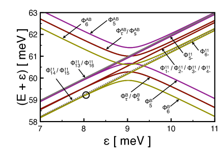
Figure 9: (color online) Two particle spectrum at $B=0$ as a function of detuning $\varepsilon$ demonstrating a gradual transition between the $(11)$ and $(02)$ configurations. Parameter values are the same as in Fig. 3(b), dielectric constant $\kappa=10$. Hybridized bonding and antibonding states are designated as $\Phi^{B}_{i}=\alpha_{i}\Phi_{i+}^{11}+\beta_{i}\Phi_{i}^{02}$ and $\Phi_{i}^{AB}=\alpha_{i}\Phi_{i+}^{11}-\beta_{i}\Phi_{i}^{02}$, respectively. The coefficients $\alpha_{i},\beta_{i}>0$ depend on $\varepsilon$ and were found from numerical diagonalization. Antisymmetric $|\Phi^{11}\rangle$ states that practically do not hybridize with $|\Phi^{02}\rangle$ states are designated as $|\Phi^{11}_{i-}\rangle$. Slashes indicate the states that are either exactly (Kramers) or nearly degenerate; all of them are spin (isospin) polarized. The states $|\Phi_{5}\rangle$ and $|\Phi_{6}\rangle$ are split by SO coupling. Remarkably, the ground states of $(02)$ and $(11)$ are not tunnel coupled, and the circle highlights the crossing point between the states $|\Phi^{B}_{6}\rangle$ and $|\Phi^{11}_{6-}\rangle$

.

One general comment regarding the ground states of two-electron DQDs is relevant. According to the Lieb-Mattis theorem,LM ; AM the ground state of a two-electron system, at $B=0$ and in the absence of SO coupling, is always a spin singlet. The proof of this statement (attributed to Wigner in Ref. LM, ) is applicable only to scalar wave functions. Therefore, it is not applicable to carbon nanotubes where the wave functions are spinors in the pseudospin space. Also, the classification of the quantum states of SO coupled systems is generically impossible in terms of the spin eigenstates. Hence, it is quite remarkable that despite all these odds, both GS wave functions of Fig. 9 belong to the group of functions with zero mean value of the spin. A specific GS function is chosen by a number of competing parameters.

Fig. 10 presents the energy spectrum as a function of detuning $\varepsilon$ for a magnetic field $B=1$ T. All degeneracies, both in $(11)$ and $(02)$, are lifted. This field is large enough to change the symmetry of the ground states both in the $(11)$- and $(02)$- configurations. Once again, a GS to GS transition is not allowed. At the $(02)$ side, the splitting of the isospin doublet $|\Phi_{\tau}^{02}\rangle$, $\tau=\pm 1$, becomes larger than the SO splitting separating $|\Phi^{02}_{5}\rangle$ and $|\Phi^{02}_{6}\rangle$ states and its $\tau=+$ component $|\Phi^{02}_{3}\rangle$ shifts to the spectrum bottom, in agreement with the experimental findings of Refs. Kuemmeth, and Churchill, . At the $(11)$ side, the magnetic field splits the $|\Phi^{11}_{14,15}\rangle$ Kramers doublet (that was only slightly above the ground state in Fig. 9) and shifts its $\mid\Phi_{14}\rangle$ component to the spectrum bottom; it is spin and isospin polarized with $s=\downarrow,\tau=+$. In this context, it is instructive to follow the adiabatic evolution of the $|\Phi^{B}_{3}\rangle$ ground state starting from $|\Phi^{02}_{3}\rangle$ in the lower right corner of Fig. 10. After crossing the $|\Phi_{14}\rangle$ ground state (this crossing is both spin conservation and $L/R$ symmetry protected), it passes through a narrow anticrossing with $|\Phi^{11}_{3-}\rangle$ (protected by the weak $B$ dependence of $\eta_{\tau,s}(B)$ and highlighted by a circle) to appear only slightly above it as $|\Phi^{11}_{3+}\rangle$, see Fig. 11. Similarly to the related comment to Fig. 9, the width of the avoided crossing can be enhanced by producing asymmetry between the left and right dots. Since $|\Phi^{11}_{14}\rangle$ and both states $|\Phi^{11}_{3\pm}\rangle$ possess the same pseudospin $\tau=+$ while $|\Phi^{11}_{3\pm}\rangle$ are spin unpolarized and $|\Phi^{11}_{14}\rangle$ is spin polarized, the relaxation from $|\Phi^{11}_{3\pm}\rangle$ to the ground state is only possible due to the spin nonconservation. Therefore, excursions from $(02)$ to $(11)$ can be used for measuring the spin relaxation rate.

Figure 10: (color online) Same as in Fig. 9 for a magnetic field $B=1$ T. Again, bonding and antibonding states are denoted as $\Phi_{i}^{B}$ and $\Phi_{i}^{AB}$, respectively. All degeneracies are removed. Four $|\Phi^{11}_{13-16}\rangle$ states and six $|\Phi^{11}_{i-}\rangle$ that practically do not hybridize with $|\Phi^{02}\rangle$ states are shown as ascending lines. The circle highlights the intersection of the $|\Phi_{3}^{B}\rangle$ hybridized state with $|\Phi^{11}_{3-}\rangle$. See text for details.

We have checked the behavior of the level crossings, highlighted by circles in Figs. 9 and 10, when we change the size of the gap $E_{g}$. With $E_{g}$ increasing twice, both crossings remain stable and move to the right, nearly half way to the $(11)$-$(02)$ degeneracy point ($\varepsilon\sim 11$ meV).

In Figs. 9 and 10, in the vicinity of the $(11)$-$(02)$ degeneracy point, gross features are dominated by the $|\Phi^{11}\rangle$ - $|\Phi^{02}\rangle$ hybridization. To illuminate different properties of the spectrum, its SO-coupling and $B$-dependence, we present in Fig. 11 the energy spectrum at $\varepsilon=2$ meV. While it was found by the same procedure as Figs. 9 and 10, we checked that it is very close to the spectrum found in the $16\times 16$ basis of $|\Phi^{11}\rangle$ functions; in particular, all levels follow in the same order. This proves that the contribution of the polar configuration $(20)$ (with both electrons on the left dot) not included in our calculations is small at $\varepsilon=2$ meV and has only minor effect on the results.

At $B=0$, the spectrum is dominated by the splitting originating from the one- or two-fold population of the upper and lower Kramers doublets separated by $\Delta_{SO}\sim 0.4$ meV. Splittings from the inter-dot exchange matrix elements are lesser: $J_{LR}^{i}\approx 0.03$ meV for $\kappa=10$, Fig. 11. The tunneling matrix elements $\eta\sim 0.02$ meV [see Fig. 5 and Eq. (60)] also induce lesser splittings. Therefore, the gross structure of the energy spectrum is controlled by $\Delta_{SO}$, and this suggests describing it primarily in terms of Kramers doublets rather than independent spin and isospin populations. The fine structure inside each group (4+8+4), originating from tunneling and Coulomb terms, should be accessible for experimental resolution. One can also distinguish energy differences between the bonding and antibonding $|\Phi^{11}_{i\pm}\rangle$ states and the states forbidden for tunneling to $(02)$. It is seen that the energies of antisymmetric states are lower than the energies of the corresponding symmetric states in the whole range of magnetic fields. This is the result of the Coulomb interaction that favors antisymmetric states prevailing over tunneling that favors symmetric states.

The $B$-dependence is dominated by the isospin Zeeman coupling because $\mu_{orb}\gg\mu_{B}$. However, more careful examination allows distinguishing differences in the slopes of the states with the spin and isospin polarized in the same or in opposite directions, e.g., $|\Phi^{11}_{15,16}\rangle$. A Zeeman splitting of spin polarized states $|\Phi^{11}_{1\pm,2\pm}\rangle$ is distinctly seen.

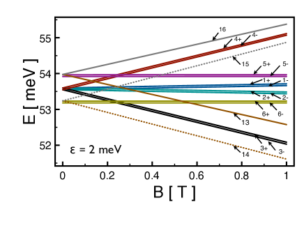
Figure 11: (color online) Magnetic field dependence of the energy spectrum of a two-electron double dot for $\varepsilon=2$ meV where the admixture of both $(02)$ and $(20)$ configurations is negligibly small. The Coulomb interaction is screened by $\kappa=10$ and other parameters are the same as in Fig. 3. Numbers with arrows denote particular $\mid\Phi^{11}_{1\pm,\dots,6\pm,14,\dots,16}\rangle$ states. Relative magnitudes of the different level splittings originating from the tunneling and Coulomb interaction are distinctly seen. At $B=0$, the dominating splitting comes from $\Delta_{SO}$ depending on whether one or both electrons belong to the upper or lower Kramers doublet; other contributions are smaller by one order of magnitude. The strong $B$ dependence is controlled by the isospin through $\mu_{orb}$ and a weaker one by the spin through $\mu_{B}$. The splittings of bonding and antibonding levels are weak, and their sign is controlled by the prevalence of the Coulomb contribution over tunneling.

V Summary and discussion

We have studied the detailed structure of the energy spectrum of a symmetric carbon nanotube double quantum dot with either one or two electrons confined by an electrostatic potential. We focused on narrow-gap coated nanotubes allowing efficient gate control for electronic and spintronic applications, and investigated the effect of both SO coupling constants, $\Delta_{0}$ and $\Delta_{1}$, on the energy spectrum. The large effective dielectric constant of such nanotubes ($\kappa\sim 10$) in conjunction with a small electron effective mass $m^{*}\approx E_{g}/v^{2}$ suppresses admixture of the higher longitudinal modes and allows studying the fine structure of the spectrum originating from the spin and isospin degrees of freedom in the framework of a single-mode theory. The importance of such a study is called for by the experimental discoveryChurchill2 ; Churchill of very narrow features ($\lesssim 10$ mT) in the magnetotransport spectra of DQDs. While a recent theoryBurkard proposed a mechanism for developing magnetocurrent minima with a width $\Delta_{SO}/\mu_{orb}\sim 100$ mT based on the global width $\Delta_{SO}$ of the SO split spectrum, unveiling the nature of the narrow features seem to require mechanisms involving specific quantum levels. Note that the basic elements of our theory are also applicable to suspended semiconducting nanotubes as well, but accounting for higher longitudinal modes might become necessary.Wunsch ; Rontani ; Stecher

After solving a spinor equation for a double square-well confining potential in the axial direction, we obtained the single-particle spectrum in the presence of SO interaction. Due to the coupling between spin and isospin, the four-fold degeneracy is lifted at zero magnetic field, $B=0$, which results in two Kramers doublets corresponding to either aligned or anti-aligned spin and isospin. We note that while the diagonal $\Delta_{0}$ and nondiagonal $\Delta_{1}$ SO coupling constants combine in the splitting $\Delta_{SO}$ between the Kramers doublets, $\Delta_{1}$ contributes independently to the interdot tunneling rate. As a result, Kramers doublets acquire different $B$-dependent tunneling rates, Fig. 5; we estimated this difference using the realistic values of $\Delta_{0}$ and $\Delta_{1}$ found from the experimental data of Ref. Kuemmeth, . They can be observed in experiments on single-electron transport across double dots.

The basis states for a two-electron DQD in the $(02)$ configuration (both electrons on the right dot) include two spin polarized as well as two isospin polarized functions, and two functions belonging to the upper and lower Kramers doublet, respectively. All of them are spin-isospin coupled, and the Coulomb interaction energies depend both on the spin and isospin. In the $(11)$ configuration of a symmetric DQD, these functions generate (by moving a single electron from the right to the left dot) 12 basis functions of which 6 are symmetric (bonding) and 6 antisymmetric (antibonding) in the indices of the left $(L)$ and right $(R)$ dots. Four more states, all $L/R$ antisymmetric, have no analogs in the $(02)$ space. Only bonding modes strongly hybridize with $(02)$ states.

Our main result is the energy spectrum of a two-electron DQD, calculated for the regime of comparable tunneling and SO energies, shown in Fig. 9 for $B=0$ and in Fig. 10 for $B=1$ T as a function of the detuning $\varepsilon$ between left and right dots. It is discussed in Sec. IV.3. Figures 9 and 10 illustrate how fundamentally the isospin degree of freedom and its coupling to the spin change the spectrum. This change makes the analysis of the spectrum much more complicated compared to the spectrum of GaAs DQDs Hanson which consists of the spin singlet and triplet branches alone.

While both the Pauli blockade and dephasing rate are challenging goals for experimental studies, investigating the dephasing rate by initializing the system in the $(02)$ configuration and making excursions into the $(11)$ configuration is more tractable from a theoretical point of view because of a lesser manifold of quantum states whose width can be controlled by gate potentials. The effect of a magnetic field on the mutual position of the lower levels that influences the relaxation rate between them can be inferred from Figs. 9 and 10 as discussed in Sec. IV.3. As distinct from GaAs where the ground state is a singlet, in nanotube DQDs this is a double-populated lower Kramers doublet. We have also found that in our parameter range the ground state in the $(11)$ configuration is antisymmetric in $L/R$ indices because the Coulomb repulsion prevails over tunneling. This unique situation results in the opposite $L/R$ parity of the ground state on both sides of the $(11)$-$(02)$ degeneracy point, Fig. 9. Therefore, low energy excursions into the $(11)$ configuration can probe the relaxation rate at small energy transfers and indicate the position of the $L/R$ symmetry point (deviation from it turns the level crossing into an anticrossing). When the magnetic field becomes strong enough, Zeeman splitting shifts a spin polarized state to the bottom of the spectrum. As a result, ground states on the left and right differ not only in the $L/R$ symmetry but also in the two-particle spin wavefunction, Fig. 10. Hence, similar excursions can probe the spin relaxation rate $\tau^{-1}_{s}$. Moving up in energy should allow probing higher states of the $(11)$ configuration.

With such a rich energy spectrum, the very notion of the spin (Pauli) blockade should be generalized,Churchill including both spin and isospin, and the blockade becomes rather sensitive to the parameters of the system. Therefore, it is natural that the blockade has either been observedChurchill or alternatively not observedKouwenhoven by different experimental groups. The outcome should strongly depend on populating the different $(11)$ levels during the initiation phase, mechanisms of the relaxation and leakage, and the topology of the dense intertwined net of the energy levels. A significant challenge is establishing the optimal conditions for achieving the Pauli blockade.

The pattern of the energy spectrum, which is rather involved even in the framework of a simple model (Fig. 10) should become even more complicated in realistic systems due to the $\tau$ non-conservation that is usually controlled by extrinsic mechanisms and, therefore, might be different in the left and right dots. It can be taken into account either phenomenologically by including a term $\Delta_{KK^{\prime}}\tau_{1}$ into the Hamiltonian,Churchill ; Bulaev ; Rudner ; Marcus or by modeling a short-range disorder.Burkard Likewise, the electron attraction through their coupling to stretching phonons that can compete with the Coulomb repulsion at $\kappa\sim 10$, cf. Sec. III.3, is not studied here and deserves a detailed investigation in the future.

Note added: While completing this manuscript, we became aware of a paper by v. Stecher et al.Stecher on a related subject. Both studies are complementary, since Ref. Stecher, focuses mostly on the effect of electronic correlations in suspended wide-gap nanotubes, while we concentrate on the fine SO structure of the spectra of coated narrow-gap nanotubes where such correlations are suppressed.

- (1) R. Hanson, L. P. Kouwenhoven, J. R. Petta, S. Tarucha, and L. M. K Vandersypen, Rev. Mod. Phys. 79, 1217 (2007).
- (2) J. R. Petta, A. C. Johnson, J. M. Taylor, E. A. Laird, A. Yacoby, M. D. Lukin, C. M. Marcus, M. P. Hanson, and A. C. Gossard, Science 309, 2180 (2005).
- (3) S. Iijima, Nature (London) 354, 56 (1991).
- (4) F. Kuemmeth, H. O. H. Churchill, P. K. Herring, and C. M. Marcus, Mater. Today 13, 18 (2010).
- (5) H. O. H. Churchill, A. J. Bestwick, J. W. Harlow, F. Kuemmeth, D. Marcos, C. H. Stwertka, S. K. Watson, and C. M. Marcus, Nat. Phys. 5, 321 (2009).
- (6) R. Saito, G. Dresselhaus, M. S. Dresselhaus, Physical Properties of Carbon Nanotubes, Imperial College Press, London (1998).
- (7) A. H. Castro Neto, F. Guinea, N. M. R. Peres, K. S. Novoselov, and A. K. Geim, Rev. Mod. Phys. 81, 109 (2009).
- (8) J. C. Charlier, X. Blase, S. Roche, Rev. Mod. Phys. 79, 677 (2007).
- (9) T. Ando, J. Phys. Soc. Jpn. 74, 777 (2005).
- (10) C. L. Kane, and E.J. Mele, Phys. Rev. Lett. 78, 1932 (1997).
- (11) J. W. Mintmire, B.I. Dunlap, and C.T. White, Phys. Rev. Lett. 68, 631 (1992).
- (12) N. Hamada, S. Sawada, and A. Oshiyama, Phys. Rev. Lett. 68, 1579 (1992).
- (13) R. Saito, M. Fujita, G. Dresselhaus, and M. Dresselhaus, Appl. Phys. Lett. 60, 2204 (1992).
- (14) A. Kleiner, S. Eggert, Phys. Rev. B 63, 73408 (2001), ibid. 64, 113402 (2001).
- (15) G. A. Steele, G. Gotz, and L. P. Kouwenhoven, Nat. Nanotechnologies 4, 363 (2009).
- (16) P. Jarillo-Herrero, S. Sapmaz, C. Dekker, L.P. Kouwenhoven, and H.S.J. van der Zant, Nature 429, 389 (2004).
- (17) E. D. Minot, Y. Yaish, V. Sazonova, and P. L. McEuen, Nature 428, 536 (2004).
- (18) F. Kuemmeth, S. Ilani, D. C. Ralph, and P. L. McEuen. Nature 452, 448 (2008).
- (19) R. Leturcq, C. Stamper, K. Inderbitzin, L. Durrer, C. Heirold, E. Mariani, M. G. Schultz, F. von Oppen, and K. Ensslin, Nature Physics 5, 327 (2009).
- (20) H. O. H. Churchill, F. Kuemmeth, J. W. Harlow, A. J. Bestwick, E. I. Rashba, K. Flensberg, C. H. Stwertka, T. Taychatanapat, S. K. Watson, and C. M. Marcus, Phys. Rev. Lett. 102, 166802 (2009).
- (21) H. Min, J .E. Hill, N. A. Sinitsyn, B. R. Sahu, L. Kleinmann, and A. H. MacDonald, Phys. Rev. B 74, 165310 (2006).
- (22) Y. Yao, F. Ye, X. Qi, S. Zhang, and Z. Fang, Phys. Rev. B 75, 041401 (2007).
- (23) J. C. Boettger and S. B. Trickey, Phys. Rev. B 75, 121402(R) (2007), ibid. 75, 199903 (2007).
- (24) M. Gmitra, S. Konschuh, C. Ertler, C. Ambrosch-Draxl, and J. Fabian, Phys. Rev. B 80, 235431 (2009).
- (25) M. V. Entin and L. I. Magarill, Phys. Rev. B 64, 085330 (2001).
- (26) E. N. Bulgakov and A. F. Sadreev, Phys. Rev. B 66, 075331 (2002).
- (27) T. Ando, J. Phys. Soc. Jpn. 69, 1757 (2000).
- (28) A. De Martino, R. Egger, K. Hallberg, C.A. Balseiro, Phys. Rev. Lett. 88, 206402 (2002).
- (29) L. Chico, M. P. Lopez Sancho, M. C. Munoz, Phys. Rev. Lett. 93, 176402 (2004).
- (30) H. Huertas-Hernando, F. Guinea, A. Brataas, Phys. Rev. B 74, 155426 (2006).
- (31) W. Izumida, K. Sato, and R. Saito, J. Phys. Soc. Jpn. 78, 074707 (2009).
- (32) Jae-Seung Jeong, and Hyun-Woo Lee, Phys. Rev. B 80, 075409 (2009).
- (33) L. Chico, M. P. Lopez-Sancho, and M.C. Munoz, Phys. Rev. B 79, 235423 (2009).
- (34) D. V. Bulaev, B. Trauzettel, and D. Loss, Phys. Rev. B 77, 235301 (2008).
- (35) B. Wunsch, Phys. Rev. B 79, 1 (2009).
- (36) A. Secchi, and M. Rontani, Phys. Rev. B 80, 041404(R) (2009), ibid. 82, 035417 (2010).
- (37) J. Fischer, B. Trauzettel, and D. Loss, Phys. Rev. B 80, 155401 (2009).
- (38) A. Pályi, and G. Burkard, Phys. Rev. B 80, 201404(R) (2009) and arXiv:1005.2738 (2010).
- (39) D. Culcer, L. Cywinski1, Q. Li, X. Hu, and S. Das Sarma , Phys. Rev. B 80, 205302 (2009).
- (40) C. L. Kane and E. J. Mele, Phys. Rev. Lett. 95, 226801 (2005).
- (41) A. M. Lunde, K. Flensberg, and A.-P. Jauho, Phys. Rev. B 71, 125408 (2005).
- (42) C. T. White, D. H. Robertson, and J. W. Mintmire, Phys. Rev. B 47, 5485 (1993).
- (43) W. G. van der Wiel, S. De Franceschi, J. M. Elzerman, T. Fujisawa, S. Tarucha, and L. P. Kouwenhoven, Rev. Mod. Phys. 75, 1 (2002).
- (44) J. von Stecher, B. Wunsch, M. Lukin, E. Demler, and A.M. Rey, arXiv:1006.0209 (2010).
- (45) M. S. Rudner and E. I. Rashba, Phys. Rev. B 81, 125426 (2010).
- (46) L. D. Landau and E. M. Lifshitz, Quantum Mechanics, (Pergamon, Oxford) 1977, § 62.
- (47) S. H. Jhang, M. Marganska, Y. Skourski, D. Preusche, B. Witkamp, M. Grifoni, H. van der Zant, J. Wosnitza, and C. Strunk, Phys. Rev. B 82, 041404(R) (2010).
- (48) R. Egger, A.O. Gogolin, Phys. Rev. Lett. 79, 5082 (1997), Eur. Phys. J. B 3, 281 (1998).
- (49) E. Lieb and D. Mattis, Phys. Rev. 125, 164 (1962).
- (50) N. W. Ashcroft and N. D. Mermin, Solid State Physics, Saunders College Publishing, Orlando (1976), Chap. 32.
- (51) K. Flensberg and C. M. Marcus, Phys. Rev. B 81, 195418 (2010).