Riemannian optimization
on tensor products of Grassmann manifolds: Applications to generalized Rayleigh-quotients

Abstract

We introduce a generalized Rayleigh-quotient $\rho_{A}$ on the tensor product of Grassmannians $\mathrm{Gr}^{\otimes r}({\bf m},{\bf n})$ enabling a unified approach to well-known optimization tasks from different areas of numerical linear algebra, such as best low-rank approximations of tensors (data compression), geometric measures of entanglement (quantum computing) and subspace clustering (image processing). We briefly discuss the geometry of the constraint set $\mathrm{Gr}^{\otimes r}({\bf m},{\bf n})$, we compute the Riemannian gradient of $\rho_{A}$, we characterize its critical points and prove that they are generically non-degenerated. Moreover, we derive an explicit necessary condition for the non-degeneracy of the Hessian. Finally, we present two intrinsic methods for optimizing $\rho_{A}$ — a Newton-like and a conjugated gradient — and compare our algorithms tailored to the above-mentioned applications with established ones from the literature.

1 Introduction

The present paper addresses a constrained optimization problem, subsuming and extending optimization tasks which arise in various areas of applications such as (i) low-rank tensor approximation problems from signal processing and data compression, (ii) geometric measures of pure state entanglement from quantum computing, (iii) subspace reconstruction problems from image processing and (iv) combinatorial problems.

The problem can be stated as follows: Given a collection of integer pairs $(m_{j},n_{j})$ with $1\leq m_{j}\leq n_{j}$ for $j=1,\dots,r$ and a Hermitian $N\times N$ matrix $A$ with $N:=n_{1}n_{2}\cdots n_{r}$, find the global maximizer of the trace function ${\bf P}\mapsto\operatorname{tr}(A{\bf P})$. Here, ${\bf P}$ is restricted to the set of all Hermitian projectors ${\bf P}:{\mathbb{C}}^{N}\to{\mathbb{C}}^{N}$ of rank $M:=m_{1}m_{2}\cdots m_{r}$, which can be represented as a tensor product ${\bf P}:=P_{1}\otimes\dots\otimes P_{r}$ of Hermitian projectors $P_{j}:{\mathbb{C}}^{n_{j}}\to{\mathbb{C}}^{n_{j}}$ of rank $m_{j}$. Thus, one is faced with the constrained optimization task

$$\max\operatorname{tr}(A{\bf P})\quad\textrm{subject to}\;{\bf P}\in\mathrm{Gr}^{\otimes r}({\bf m},{\bf n}),$$ (1)

where $\mathrm{Gr}^{\otimes r}({\bf m},{\bf n})$ denotes the set of all Hermitian projectors of the above tensor type and $({\bf m},{\bf n})$ is a shortcut for $\big{(}(m_{1},n_{1}),\dots,(m_{r},n_{r})\big{)}$. We will see that it makes sense to call the above objective function ${\bf P}\mapsto\operatorname{tr}(A{\bf P})=:\rho_{A}({\bf P})$ the generalized Rayleigh-quotient of $A$ with respect to the partitioning $({\bf m},{\bf n})$.

To the best of the authors’ knowledge, problem (1) has not been discussed in the literature in this general setting. However, depending on the structure of $A$ as well as on the choice of $({\bf m},{\bf n})$, problem (1) relates to well-known numerical linear algebra issues:

(i) For Hermitian matrices of rank-$1$, i.e. $A=vv^{\dagger}$, it reduces to a best low-rank approximation problem for the tensor $\mathcal{A}\in{\mathbb{C}}^{n_{1}\times n_{2}\times\dots\times n_{r}}$ which satisfies $v=\mathrm{vec}(\mathcal{A})$, cf. [21, 28]. Classical application areas of such low-rank approximations can be found in statistics, signal processing and data compression [4, 20, 21, 31].

(ii) A recent application in quantum computing plays a central role in characterizing and quantifying pure state entanglement. Here, the distance of a pure state (tensor) to the set of all product states (rank-$1$ tensors) provides a geometric measure for entanglement [6, 23, 34].

(iii) Moreover, the challenging task of recovering subspaces of possibly different dimensions from noisy data — known as subspace detection or subspace clustering problem in computer vision and image processing [33] — can also be cast into the above setting. More precisely, for an appropriately chosen Hermitian matrix $A$ the subspace clustering task can be characterized by problem (1) in the sense that for unperturbed data the global minima of the generalized Rayleigh-quotient are in unique correspondence with the sought subspaces. Numerical experiments in Section 4 support that even for noisy data the proposed optimization yields reliable approximations of the unperturbed subspaces.

(iv) In [3] a certain class of combinatorial problems are recast as optimization problems for trace functions on the special unitary group. For the case when $A$ is a diagonal matrix, optimization task (1) is a generalization of the applications mentioned in [3].

Our solution to problem (1) is based on the fact that the constraint set $\mathrm{Gr}^{\otimes}({\bf m},{\bf n})$ can be equipped with a Riemannian submanifold structure. This admits the use of techniques from Riemannian optimization — a rather new approach towards constrained optimization exploiting the geometrical structure of the constraint set in order to develop numerical algorithms [1, 14, 32]. In particular, we pursue two approaches: a Newton and a conjugated gradient method.

On a Riemannian manifold, the intrinsic Newton method is usually described by means of the Levi-Civita connection, performing iterations along geodesics, see [9, 29]. A more general approach via local coordinates was initiated by Shub in [27] and further discussed in [1, 13]. Here, we follow the ideas in [13] and use a pair of local parametrizations — normal coordinates for the push-forward and QR-type coordinates for the pull-back — satisfying an additional compatibility condition to preserve quadratic convergence. Thus we obtain an intrinsically defined version of the classical Newton algorithm with some computational flexibility. Nevertheless, for high-dimensional problems its iterations are expensive, both in terms of computational complexity and memory requirements. Therefore, we alternatively propose a conjugated gradient method, which has the advantage of algorithmic simplicity at a satisfactory convergence rate. In doing so, we suggest to replace the global line-search of the classical conjugated gradient method by a one-dimensional Newton-step, which yields a better convergence behavior near stationary points than the commonly used Armijo-rule.

As mentioned earlier, depending on the structure of $A$, the above-specified problems (i), (ii), (iii) and (iv) are particular cases of the optimization task (1). For the best low-rank approximation of a tensor the standard numerical approach is an alternating least-squares algorithm, known as higher-order orthogonal iteration (HOOI) [21]. Recently, several new methods also exploiting the geometric structure of the problem have been published. Newton algorithms have been proposed in [8, 18], quasi-Newton methods in [28], conjugated gradient and trust region methods in [17]. For high-dimensional tensors, all Riemannian Newton algorithms manifest similar problems: too high computational complexity and memory requirements. Our conjugated gradient method is however, a good candidate to solve large scale problems. It exhibits locally a good convergence behavior, comparable to that of the quasi-Newton methods in [28] at much lower computational costs, which considerably reduces the necessary CPU time.

For the problem of estimating a mixture of linear subspaces from sampled data points, cf. (iii), our numerical approach is an efficient alternative to the classical ones: ad-hoc type methods such as K-subspace algorithms [16], or probabilistic methods using a Maximum Likelihood framework for the estimation [30].

The paper is organized as follows. In Section 2, we familiarize the reader with the basic ingredients of Riemannian optimization. In particular, we address the following topics: the Riemannian submanifold structure of the constraint set $\mathrm{Gr}^{\otimes r}({\bf m},{\bf n})$, its isometry to the $r$-fold cartesian product of Grassmannians, geodesics and parallel transport and the computation of the intrinsic gradient and Hessian for smooth objective functions. Section 3 is dedicated to the problem of optimizing the generalized Rayleigh-quotient $\rho_{A}$, including also a detailed discussion on its relation to problems (i), (ii), (iii) and (iv). Moreover, an analogy to the classical Rayleigh-quotient is also the subject of this section. We compute the gradient and the Hessian of the generalized Rayleigh-quotient and derive critical point conditions. We end the section with a result on the generic non-degeneracy of its critical points. In Section 4, a Newton-like and a conjugated gradient algorithm as well as numerical simulations tailored to the previously mentioned applications are given.

2 Preliminaries

2.1 Riemannian structure of $\mathrm{Gr}^{\otimes r}({\bf m},{\bf n})$

We start our study on the optimization task (1) with a brief summary on the necessary notations and basic concepts.

Let $\mathfrak{her}_{n}$ be the set of all Hermitian $n\times n$ matrices $A$, i.e. $A\in{\mathbb{C}}^{n\times n}\;\textrm{with}\;A^{\dagger}=A$, where $A^{\dagger}$ refers to the conjugate transpose of $A.$ Moreover, let $\mathrm{SU}_{n}$ be the Lie group of all special unitary matrices and $\mathfrak{su}_{n}$ its Lie-algebra, i.e. $\Theta\in\mathrm{SU}_{n}$ if and only if $\Theta^{\dagger}\Theta=I_{n},\;\mathrm{det}\Theta=1$ and, respectively, $\Omega\in\mathfrak{su}_{n}$ if and only if $\Omega^{\dagger}=-\Omega$ and $\operatorname{tr}(\Omega)=0.$ The Grassmannian,

$$\mathrm{Gr}_{m,n}:=\{P\in{\mathbb{C}}^{n\times n}\;|\;P=P^{\dagger}=P^{2},\;\operatorname{tr}(P)=m\},$$ (2)

is the set of all rank $m$ Hermitian projection operators of ${\mathbb{C}}^{n}$. It is a smooth and compact submanifold of $\mathfrak{her}_{n}$ with real dimension $2m(n-m)$, whose tangent space at $P$ is given by

$$\mathrm{T}_{P}\mathrm{Gr}_{m,n}=\{[P,\Omega]:=P\Omega-\Omega P\;|\;\Omega\in\mathfrak{su}_{n}\},$$ (3)

cf. [13]. Hence, every element $P\in\mathrm{Gr}_{m,n}$ and every tangent vector $\xi\in\mathrm{T}_{P}\mathrm{Gr}_{m,n}$ can be written as

$$P=\Theta\Pi_{m,n}\Theta^{\dagger}\;\;\textrm{and}\;\;\xi=\Theta\zeta_{m,n}\Theta^{\dagger},$$ (4)

where $\Pi_{m,n}$ is the standard projector of rank $m$ acting on ${\mathbb{C}}^{n}$ and $\zeta_{m,n}$ denotes a tangent vector in the corresponding tangent space, i.e.

$$\begin{array}[]{cc}\Pi_{m,n}=\left[\begin{array}[]{cc}I_{m}&0\\ 0&0\end{array}\right],&\zeta_{m,n}=\left[\begin{array}[]{cc}0&Z\\ Z^{\dagger}&0\end{array}\right],\;\;Z\in{\mathbb{C}}^{m\times(n-m)}.\end{array}$$ (5)

Whenever the values of $m$ and $n$ are clear from the context, we will use the shortcuts $\Pi$ and $\zeta$. With respect to the Riemannian metric induced by the Frobenius inner product of $\mathfrak{her}_{n}$, the Grassmannian $\mathrm{Gr}_{m,n}$ is a Riemannian submanifold and the unique orthogonal projector onto $\mathrm{T}_{P}\mathrm{Gr}_{m,n}$ is given by

$$\mathrm{ad}^{2}_{P}X=[P,[P,X]],\;\;\;X\in\mathfrak{her}_{n}.$$ (6)

We define the $r-$fold tensor product of Grassmannians $\mathrm{Gr}_{m_{j},n_{j}},\;j=1,\dots,r$ as the set

$$\mathrm{Gr}^{\otimes r}({\bf m},{\bf n}):=\displaystyle\{P_{1}\otimes\dots\otimes P_{r}\;|\;P_{j}\in\mathrm{Gr}_{m_{j},n_{j}},\;j=1,\dots,r\}$$ (7)

of all rank-$M$ Hermitian projectors of $\mathbb{C}^{N}$ with $M:=m_{1}m_{2}\cdots m_{r}$ and $N:=n_{1}n_{2}\cdots n_{r}$, which can be represented as a Kronecker product $P_{1}\otimes\dots\otimes P_{r}.$ Here, $({\bf m},{\bf n})$ stands for the multi index

$$({\bf m},{\bf n}):=\Big{(}(m_{1},n_{1}),(m_{2},n_{2}),\dots,(m_{r},n_{r})\Big{)}.$$ (8)

Then, $\mathrm{Gr}^{\otimes r}({\bf m},{\bf n})$ can be naturally equipped with a submanifold structure as the following result shows.

Proposition 2.1.

The $r-$fold tensor product of Grassmannians $\mathrm{Gr}^{\otimes r}({\bf m},{\bf n})$ is a smooth and compact submanifold of $\mathfrak{her}_{N}$ of real dimension $2\displaystyle\sum\limits_{i=1}^{r}m_{i}(n_{i}-m_{i})$.

Proof.

We consider the following smooth action

$$\begin{array}[]{cc}\sigma:\mathrm{SU}({\bf n})\times\mathfrak{her}_{N}\rightarrow\mathfrak{her}_{N},&({\boldsymbol{\Theta}},Y)\mapsto{\boldsymbol{\Theta}}Y{\boldsymbol{\Theta}}^{\dagger},\end{array}$$

of the compact Lie group

$$\mathrm{SU}({\bf n}):=\{{\boldsymbol{\Theta}}:=\displaystyle\Theta_{1}\otimes\dots\otimes\Theta_{r}\;|\;\Theta_{j}\in\mathrm{SU}_{n_{j}}\}\subset\mathrm{SU}_{N}.$$ (9)

Let $X\in\mathfrak{her}_{N}$ be of the form $X:=\displaystyle\Pi_{1}\otimes\cdots\otimes\Pi_{r},$ where $\Pi_{j}$ denotes the standard projector in $\mathrm{Gr}_{m_{j},n_{j}}.$ Then, the orbit $\mathcal{O}(X):=\{{\boldsymbol{\Theta}}X{\boldsymbol{\Theta}}^{\dagger}|\;{\boldsymbol{\Theta}}\in\mathrm{SU}({\bf n})\}$ of $X$ coincides with $\mathrm{Gr}^{\otimes r}({\bf m},{\bf n})$. By [14] (pp. 44–46) we conclude that the $r-$fold tensor product of Grassmannians is a smooth and compact submanifold of $\mathfrak{her}_{N}$. Moreover, $\mathcal{O}(X)\cong\mathrm{SU}({\bf n})/\mathrm{Stab}(X)$, where the stabilizer subgroup of $X$ is given by

$$\begin{array}[]{ll}\mathrm{Stab}(X)&:=\{{\boldsymbol{\Theta}}\in\mathrm{SU}({\bf n})\;|\;{\boldsymbol{\Theta}}X{\boldsymbol{\Theta}}^{\dagger}=X\}\\[2.84526pt] &=\{{\boldsymbol{\Theta}}\in\mathrm{SU}({\bf n})\;|\;\Theta_{j}\Pi_{j}\Theta_{j}^{\dagger}=\Pi_{j},\;j=1,\dots,r\}.\end{array}$$

It follows easily that the dimension of $\mathrm{Stab}(X)$ is $\displaystyle\sum\limits_{i=1}^{r}\,[m_{i}^{2}+(n_{i}-m_{i})^{2}-1]$ and therefore,

$$\mathrm{dim}~{}(\mathrm{Gr}^{\otimes r}({\bf m},{\bf n}))=\mathrm{dim}~{}\mathrm{SU}({\bf n})-\mathrm{dim}~{}\mathrm{Stab}(X)=2\displaystyle\sum\limits_{j=1}^{r}m_{j}(n_{j}-m_{j})$$

is the dimension of the $r-$fold tensor product of Grassmannians. ∎

Remark 2.2.

$(a)\;$ Let $V\otimes W$ denote the tensor product of finite dimensional vector spaces $V$ and $W$, cf. [12, 19] and let $\displaystyle X\otimes Y:V\otimes W\rightarrow V\otimes W$ be the tensor product of $X\in\mathrm{End}(V)$ and $Y\in\mathrm{End}(W),$ given by $\displaystyle v\otimes w\mapsto\displaystyle Xv\otimes Yw,$ for all $v\in V$ and $w\in W.$ Moreover, let $B_{V}$ and $B_{W}$ be bases of $V$ and $W$, respectively. Then, the matrix representation of $X\otimes Y$ with respect to the product basis $\{v\otimes w\;|\;v\in B_{V},\,w\in B_{W}\}$ of $V\otimes W$ is given by the Kronecker product of the matrix representations of $A$ and $B$ with respect to $B_{V}$ and $B_{W}$. This clarifies the relation between the “abstract” tensor product of linear maps and the Kronecker product of matrices and justifies the term “tensor product” of Grassmannians when we refer to $\mathrm{Gr}^{\otimes r}({\bf m},{\bf n})$.
$(b)\;$ It is a well-known fact that the Grassmannian $\mathrm{Gr}_{m,n}$ is diffeomorphic to the Grassmann manifold $\mathrm{Grass}_{m,n}$ of all $m-$dimensional subspaces of ${\mathbb{C}}^{n}$, cf.[14]. Therefore, $\mathrm{Gr}_{m_{1},n_{1}}\otimes\mathrm{Gr}_{m_{2},n_{2}}$ is diffeomorphic to

$$\{V_{1}\otimes V_{2}\;|\;V_{1}\in\mathrm{Grass}_{m_{1},n_{1}},\;V_{2}\in\mathrm{Grass}_{m_{2},n_{2}}\}\subset\mathrm{Grass}_{M,N},$$ (10)

where $M:=m_{1}m_{2}$ and $N:=n_{1}n_{2}.$
Both items (a) and (b) readily generalize to an arbitrary number of Grassmannians.

We conclude this subsection by pointing out an isometry between the $r-$fold tensor product of Grassmannians $\mathrm{Gr}^{\otimes r}({\bf m},{\bf n})$ and the direct $r-$fold product of Grassmannians

$$\mathrm{Gr}^{\times r}({\bf m},{\bf n}):=\{(P_{1},\dots,P_{r})\;|\;P_{j}\in\mathrm{Gr}_{m_{j},n_{j}},\;j=1,\dots,r\}.$$ (11)

The vector spaces $\mathfrak{her}_{N}$ and $\mathfrak{her}_{n_{1}}\times\dots\times\mathfrak{her}_{n_{r}}$ endowed with the inner products

$$\langle X,Y\rangle:=\operatorname{tr}(XY)$$ (12)

and

$$\Bigl{<}(X_{1},\dots,X_{r}),(Y_{1},\dots,Y_{r})\Bigr{>}:=\operatorname{tr}(X_{1}Y_{1})+\dots+\operatorname{tr}(X_{r}Y_{r}),$$ (13)

induce a Riemannian submanifold structure on $\mathrm{Gr}^{\otimes r}({\bf m},{\bf n})$ and $\mathrm{Gr}^{\times r}({\bf m},{\bf n})$, respectively.

Proposition 2.3.

The map

$$\begin{array}[]{cc}\varphi:\mathrm{Gr}^{\times r}({\bf m},{\bf n})\rightarrow\mathrm{Gr}^{\otimes r}({\bf m},{\bf n})\;,\;\;\;(P_{1},\dots,P_{r})\mapsto P_{1}\otimes\dots\otimes P_{r}\end{array}$$ (14)

is a diffeomorphism between $\mathrm{Gr}^{\times r}({\bf m},{\bf n})$ and $\mathrm{Gr}^{\otimes r}({\bf m},{\bf n}).$ Moreover, $\varphi$ is a global Riemannian isometry when the right-hand side of (13) is replaced by

$$M_{1}\operatorname{tr}(X_{1}Y_{1})+\dots+M_{r}\operatorname{tr}(X_{r}Y_{r}),$$ (15)

with $M_{j}:=\displaystyle\prod\limits_{k=1,\;k\neq j}^{r}m_{k},$ for $j=1,\dots,r.$

Note that the isometry between $\mathrm{Gr}^{\times r}({\bf m},{\bf n})$ and $\mathrm{Gr}^{\otimes r}({\bf m},{\bf n})$ is very special, as in general the map

$$\mathfrak{her}_{n_{1}}\times\dots\times\mathfrak{her}_{n_{r}}\rightarrow\mathfrak{her}_{N},\;\;(X_{1},\ldots,X_{r})\mapsto X_{1}\otimes\cdots\otimes X_{r}$$ (16)

fails even to be injective. For the proof of Proposition 2.3 we refer to the Appendix.

2.2 Geodesics and parallel transport

It is well-known that every Riemannian manifold $\mathcal{M}$ carries a unique Riemannian or Levi-Civita connection $\boldsymbol{\nabla}$, e.g. [1, 14, 32]. By means of $\boldsymbol{\nabla}$, one defines parallel transport and geodesics as follows. Let $t\mapsto\mathcal{X}(t)$ be a vector field along a curve $\gamma$ on $\mathcal{M}$, i.e. $\mathcal{X}(t)\in\mathrm{T}_{\gamma(t)}\mathcal{M}$ for all $t\in\mathbb{R}$. Then, $\mathcal{X}$ is defined to be parallel along $\gamma$ if

$$\boldsymbol{\nabla}_{\dot{\gamma}(t)}\mathcal{X}(t)=0$$ (17)

for all $t\in\mathbb{R}$. Given $\xi\in\mathrm{T}_{\gamma(0)}\mathcal{M}$, there exists a unique parallel vector field $\mathcal{X}$ along $\gamma$ such that $\mathcal{X}(0)=\xi$ and the vector $\mathcal{X}(t)\in\mathrm{T}_{\gamma(t)}\mathcal{M}$ is called the parallel transport of $\xi$ to $\mathrm{T}_{\gamma(t)}\mathcal{M}$ along $\gamma.$ In particular, $\gamma$ is called a geodesic on $\mathcal{M}$, if $\dot{\gamma}$ is parallel along $\gamma$.

For the Grassmann manifold $\mathrm{Gr}_{m,n}$, the curve $t\mapsto\gamma(t)=e^{-t[\xi,P]}Pe^{t[\xi,P]}$ describes the geodesic through $P\in\mathrm{Gr}_{m,n}$ in direction $\xi\in\mathrm{T}_{P}\mathrm{Gr}_{m,n}$, i.e. $\gamma(t)$ satisfies equation (17) with initial conditions $\gamma(0)=P$ and $\dot{\gamma}(0)=\xi$. Similarly, it can be verified that the parallel transport of $\eta\in\mathrm{T}_{P}\mathrm{Gr}_{m,n}$ to $\mathrm{T}_{\gamma(t)}\mathrm{Gr}_{m,n}$ along the geodesic through $P$ in direction $\xi$ is given by $\eta\mapsto e^{-t[\xi,P]}\eta e^{t[\xi,P]}$. These notions can be straight-forward generalized to the direct product of Grassmannians $\mathrm{Gr}^{\times r}({\bf m},{\bf n})$.

2.3 The Riemannian gradient and Hessian

First, let us recall that the Riemannian gradient at $P\in\mathcal{M}$ of a smooth objective function $f:\mathcal{M}\to{\mathbb{R}}$ on a Riemannian manifold $\mathcal{M}$ is defined as the unique tangent vector $\mathop{\operator@font grad}\nolimits f(P)\in\mathrm{T}_{P}\mathcal{M}$ satisfying

$${\rm d}f(P)(\xi)=\langle\mathop{\operator@font grad}\nolimits f(P),\xi\rangle$$ (18)

$\textrm{for all}\;\xi\in\mathrm{T}_{P}\mathcal{M}$, where ${\rm d}f(P)$ denotes the differential (tangent map) of $f$ at $P$. Moreover, if $\boldsymbol{\nabla}$ is the Levi-Civita connection on $\mathcal{M}$, then the Riemannian Hessian of $f$ at $P$ is the linear map ${\bf H}_{f}(P):\mathrm{T}_{P}\mathcal{M}\rightarrow\mathrm{T}_{P}\mathcal{M}$ defined by

$${\bf H}_{f}(P)\xi=\boldsymbol{\nabla}_{\xi}\mathop{\operator@font grad}\nolimits f(P),$$ (19)

for all $\xi\in\mathrm{T}_{P}\mathcal{M}.$ Now, if $\mathcal{M}$ is a submanifold of a vector space $V$, then (18) and (19) simplify as follows. Let $\widetilde{f}$ and $\widetilde{\mathcal{X}}$ be smooth extensions of $f$ and of the vector field $\mathop{\operator@font grad}\nolimits f$, respectively. Then,

$$\mathop{\operator@font grad}\nolimits f(P)=\pi_{P}\big{(}\nabla\widetilde{f}(P)\big{)},\quad{\bf H}_{f}(P)\xi=\pi_{P}(D\widetilde{\mathcal{X}}(P)\xi),$$ (20)

where $\pi_{P}$ is the orthogonal projection onto $\mathrm{T}_{P}\mathcal{M}$ and $\nabla\widetilde{f}$ denotes the standard gradient of $\widetilde{f}$ on $V$.

For the generalized Rayleigh-quotient $\rho_{A}$ on $\mathrm{Gr}^{\times r}({\bf m},{\bf n})$, explicit formulas of the gradient and Hessian will be given in Section 3.3.

3 The generalized Rayleigh-quotient

Let $\mathrm{Gr}^{\otimes r}({\bf m},{\bf n})$ be the $r-$fold tensor product of Grassmannians with $({\bf m},{\bf n})$ as in (8) and let $A\in\mathfrak{her}_{N},$ $N=n_{1}n_{2}\cdots n_{r}.$ In the following, we analyze the constrained optimization problem

$$\underset{{\bf P}\in\mathrm{Gr}^{\otimes r}({\bf m},{\bf n})}{\max}\operatorname{tr}(A{\bf P}),$$ (21)

which comprises problems from different areas, such as multilinear low-rank approximations of a tensor, geometric measures of entanglement, subspace clustering and combinatorial optimization. These applications are naturally stated on a tensor product space. However, for the special case of the Grassmann manifold they can be reformulated on a direct product space. To this purpose, we define the generalized Rayleigh-quotient of the matrix $A$ as

$$\begin{array}[]{cc}\rho_{A}:\mathrm{Gr}^{\times r}({\bf m},{\bf n})\rightarrow{\mathbb{R}},&\rho_{A}(P_{1},\dots,P_{r}):=\displaystyle\operatorname{tr}\Big{(}A(P_{1}\otimes\dots\otimes P_{r})\Big{)}.\end{array}$$ (22)

Based on the isometry between $\mathrm{Gr}^{\otimes r}({\bf m},{\bf n})$ and $\mathrm{Gr}^{\times r}({\bf m},{\bf n}),$ we can rewrite problem (21) as an optimization task for $\rho_{A}$

$$\underset{(P_{1},\dots,P_{r})\in\mathrm{Gr}^{\times r}({\bf m},{\bf n})}{\max}\rho_{A}(P_{1},\dots,P_{r}).$$ (23)

In general this is not the case, as we have already pointed out in (16).

The term “generalized Rayleigh-quotient" is justified, since for $r=1$ we obtain the classical Rayleigh-quotient $\rho_{A}(P)=\operatorname{tr}(AP).$ In the sequel we want to point out some similarities and differences between the generalized and the classical Rayleigh-quotient. It is well known that under the assumption that there is a spectral gap between the eigenvalues of $A\in\mathfrak{her}_{N}$, there is a unique maximizer and a unique minimizer of the classical Rayleigh-quotient of $A$. Unfortunately, this is no longer the case for the generalized Rayleigh-quotient $\rho_{A}$. Global maximizers and global minimizers exist since the generalized Rayleigh-quotient is defined on a compact manifold, but unlike the classical case, it admits also local extrema as the following example shows. For the case when $A$ is of rank one we refer to Example 3 in [21].

Example 3.1.

Let $A=\mathrm{diag}(\lambda_{1},\lambda_{2},\lambda_{3},\lambda_{4})\in\mathfrak{her}_{4}$ be a diagonal matrix with $\lambda_{2}>\lambda_{3}>\lambda_{4}>\lambda_{1}$ and $P_{1}^{*},\;P_{2}^{*}\in\mathrm{Gr}_{1,2}$ of the form

$$\begin{array}[]{cc}P_{1}^{*}=\left[\begin{array}[]{cc}1&0\\ 0&0\end{array}\right]&\textrm{and }\;\;P_{2}^{*}=\left[\begin{array}[]{cc}0&0\\ 0&1\end{array}\right].\end{array}$$ (24)

The maximum of $\rho_{A}$ is obvious less or equal to $\lambda_{2}$. Since $\rho_{A}(P_{1}^{*},P_{2}^{*})=\lambda_{2}$, we have $(P_{1}^{*},P_{2}^{*})$ as the global maximizer of $\rho_{A}$. From (53) it follows that all $(P_{1},P_{2})\in\mathrm{Gr}_{1,2}\times\mathrm{Gr}_{1,2}$ with $P_{1}$ and $P_{2}$ diagonal, are critical points of $\rho_{A}$. In particular $(P_{2}^{*},P_{1}^{*})$ is a critical point of $\rho_{A}$ with $\rho_{A}(P_{2}^{*},P_{1}^{*})=\lambda_{3}<\lambda_{2}$. Moreover, one can check by computing the Hessian of $\rho_{A}$ at $(P_{2}^{*},P_{1}^{*})$ , see (59), that $(P_{2}^{*},P_{1}^{*})$ is actually a local maximizer of $\rho_{A}$. Comparative to the classical Rayleigh-quotient, this strange behavior results from the fact that not all $4\times 4$ permutation matrices are of the form $\Theta_{1}\otimes\Theta_{2}$, with $\Theta_{1},\;\Theta_{2}\in\mathrm{SU}_{2}$.

While for the classical Rayleigh-quotient one knows that the maximizer and minimizer are orthogonal projectors onto the space spanned by the eigenvectors corresponding to the largest and, respectively, smallest eigenvalues of $A$, it is difficult to provide an analog characterization for the global extrema of the generalized Rayleigh-quotient for an arbitrary matrix $A$. But, for particular $A$ and $r$ such a characterization is possible.
(a) If $r=2$ and $A$ is of rank one, i.e. $A=\mathrm{vec}(Y)\mathrm{vec}(Y)^{\dagger}$, with $Y\in{\mathbb{C}}^{n_{1}\times n_{2}}$, then the generalized Rayleigh-quotient can be rewritten as

$$\rho_{A}(P_{1},P_{2})=\operatorname{tr}[\mathrm{vec}(Y)\mathrm{vec}(Y)^{\dagger}(P_{1}\otimes P_{2})]=\operatorname{tr}(Y^{\dagger}P_{1}YP_{2}).$$ (25)

Under the assumption that $Y$ has full rank and distinct singular values there exist one maximizer and one minimizer. The maximizer $(P_{1}^{*},P_{2}^{*})\in\mathrm{Gr}^{\times 2}({\bf m},{\bf n})$ of $\rho_{A}$ is given by the orthogonal projectors onto the space spanned by the $m_{*}:=\min\{m_{1},m_{2}\}$ left, respective right singular vectors corresponding to the largest $m_{*}$ singular values. Similar for the minimizer, the singular vectors corresponding to the smallest $m_{*}$ singular values.
(b) If $r$ is arbitrary and $A$ diagonalizable via a transformation of $\mathrm{SU}({\bf n})=\{\Theta_{1}\otimes\cdots\otimes\Theta_{r}\;|\;\Theta_{j}\in\mathrm{SU}_{n_{j}}\}$, then we can assume without loss of generality that $A$ is diagonal. Moreover, if $A$ can be written as $\Lambda_{1}\otimes\dots\otimes\Lambda_{r},\;\textrm{with}\;\Lambda_{j}$ diagonal, which is always the case when $A=A_{1}\otimes\cdots\otimes A_{r}$, $A_{j}\in\mathfrak{her}_{n_{j}}$, then the generalized Rayleigh-quotient becomes a product of $r$ decoupled classical Rayleigh-quotients. Hence, there is one maximizer and one minimizer. However, there is a dramatic change if $A$ cannot be written as a Kronecker product of diagonal matrices. In this case $\rho_{A}$ has also local extrema, as Example 3.1 shows. From (53) one can immediately formulate the following critical point characterization.

Proposition 3.2.

Let $A\in\mathfrak{her}_{N}$ be diagonal. Then, $(P_{1},\dots,P_{r})\in\mathrm{Gr}^{\times r}({\bf m},{\bf n})$ is a critical point of $\rho_{A}$ if and only if $P_{j}$ are permutations of the standard projectors $\Pi_{j}$, for all $j=1,\dots,r$.

3.1 Applications

There is a wide range of applications for problem (23) in areas such as signal processing, computer vision and quantum information. We briefly illustrate the broad potential of (23) by four examples.

3.1.1 Best multilinear rank-$(m_{1},\dots,m_{r})$ tensor approximation

The problem of best approximation of a tensor by a tensor of lower rank is important in areas such as statistics, signal processing and pattern recognition. Unlike in the matrix case, there are several rank concepts for a higher order tensor, [21, 28]. For the scope of this paper, we focus on the multilinear rank case.

A finite dimensional complex tensor $\mathcal{A}$ of order $r$ is an element of a tensor product $V_{1}\otimes\cdots\otimes V_{r}$, where $V_{1},\dots,V_{r}$ are complex vector spaces with $\mathrm{dim}~{}V_{j}=n_{j}.$ Such an element can have various representations, a common one is the description as an $r-$way array, i.e. after a choice of bases for $V_{1},\dots,V_{r}$, the tensor $\mathcal{A}$ is identified with $\displaystyle[a_{i_{1}\dots i_{r}}]_{i_{1}=1,\dots,i_{r}=1}^{n_{1},\dots,n_{r}}\in{\mathbb{C}}^{n_{1}\times n_{2}\times\dots\times n_{r}}$, see e.g. [28]. The $j-$th way of the array is referred to as the $j-$th mode of $\mathcal{A}$. A matrix $X\in{\mathbb{C}}^{q_{j}\times n_{j}}$ acts on a tensor $\mathcal{A}\in{\mathbb{C}}^{n_{1}\times n_{2}\times\dots\times n_{r}}$ via mode$-j$ multiplication $\times_{j}$, i.e.

$$(\mathcal{A}\times_{j}X)_{i_{1}\dots i_{j-1}k_{1}i_{j+1}\dots i_{r}}=\sum\limits_{k_{2}=1}^{n_{j}}a_{i_{1}\dots i_{j-1}k_{2}i_{j+1}\dots i_{r}}x_{k_{1}k_{2}},$$ (26)

cf. [20, 28].

It is always possible to rearrange the elements of $\mathcal{A}$ along one or, more general, several modes such that they form a matrix. Let $l_{1},\dots,l_{q}$ and $c_{1},\dots,c_{p}$ be ordered subsets of $1,\dots,r$ such that $\{l_{1},\dots,l_{q}\}\cup\{c_{1},\dots,c_{p}\}=\{1,\dots,r\}$. Moreover, consider the products $N_{k}:=n_{l_{k+1}}\cdots n_{l_{q}},\;N^{\prime}_{k}:=n_{c_{k+1}}\cdots n_{c_{p}},$ for $k=0,\dots,q-1$ and $k=0,\dots,p-1$, respectively. Then, the matrix unfolding of $\mathcal{A}$ along $(l_{1},\dots,l_{q})$ is a matrix $A_{(l_{1},\dots,l_{q})}$ of size $N_{0}\times N^{\prime}_{0}$ such that the element in position $(i_{1},\dots,i_{r})$ of $\mathcal{A}$ moves to position $(s,t)$ in $A_{(l_{1},\dots,l_{q})}$, where

$$s:={i}_{l_{q}}+\sum\limits_{k=1}^{q-1}({i}_{l_{k}}-1)N_{k}\quad\quad\mbox{and}\quad\quad t:=i_{c_{p}}+\sum\limits_{k=1}^{p-1}(i_{c_{k}}-1)N^{\prime}_{k}.$$ (27)

As an example, for a third order tensor $\mathcal{A}\in{\mathbb{C}}^{2\times 2\times 2}$ we obtain the following matrix unfoldings as in [20]

$$\begin{array}[]{c}\begin{array}[]{cc}A_{(1)}=\left[\begin{array}[]{cccc}a_{111}&a_{112}&a_{121}&a_{122}\\ a_{211}&a_{212}&a_{221}&a_{222}\end{array}\right],&A_{(2)}=\left[\begin{array}[]{cccc}a_{111}&a_{112}&a_{211}&a_{212}\\ a_{121}&a_{122}&a_{221}&a_{222}\end{array}\right],\end{array}\\[8.53581pt] A_{(3)}=\left[\begin{array}[]{cccc}a_{111}&a_{121}&a_{211}&a_{221}\\ a_{112}&a_{122}&a_{212}&a_{222}\end{array}\right].\end{array}$$

The multilinear rank of $\mathcal{A}\in{\mathbb{C}}^{n_{1}\times\dots\times n_{r}}$ is the $r-$tuple $(m_{1},\dots,m_{r})$ such that

$$m_{1}=\mathrm{rank}~{}A_{(1)}\;,\;\;\dots\;\;,\;m_{r}=\mathrm{rank}~{}A_{(r)}.$$ (28)

To refer to the multilinear rank of $\mathcal{A}$ we will use the notation rank-$(m_{1},\dots,m_{r})$ or $\mathrm{rank}~{}\mathcal{A}=(m_{1},\dots,m_{r}).$ Given a tensor $\mathcal{A}\in{\mathbb{C}}^{n_{1}\times\dots\times n_{r}},$ we are interested in finding the best rank-$(m_{1},\dots,m_{r})$ approximation of $\mathcal{A}$, i.e.

$$\underset{\mathrm{rank}(\mathcal{B})\leq(m_{1},\dots,m_{r})}{\min}\|\mathcal{A}-\mathcal{B}\|.$$ (29)

Here, $\|\mathcal{A}\|$ is the Frobenius norm of a tensor, i.e. $\|\mathcal{A}\|^{2}=\langle\mathcal{A},\mathcal{A}\rangle$ with

$$\langle\mathcal{A},\mathcal{B}\rangle=\mathrm{vec}(\mathcal{A})^{\dagger}\mathrm{vec}(\mathcal{B})=\sum\limits_{i_{1},\dots,i_{r}=1}^{n_{1},\dots,n_{r}}\bar{a}_{i_{1}\dots i_{r}}b_{i_{1}\dots i_{r}}.$$ (30)

Here, $\mathrm{vec}(\mathcal{A})$ refers to the matrix unfolding $A_{(1,\dots,r)}\in\mathbb{C}^{N\times 1}$. In the matrix case, the solution of the optimization problem (29) is given by a truncated SVD, cf. Eckart-Young theorem [7]. However, for the higher-order case, there is no equivalent of the Eckart-Young theorem. According to the Tucker decomposition [31] or the higher order singular value decomposition (HOSVD) [20], any rank-$(m_{1},\dots,m_{r})$ tensor can be written as a product of a core tensor $\mathcal{S}$ and $r$ Stiefel matrices $X_{1}\in{\mathbb{C}}^{m_{1}\times n_{1}},\dots,\;X_{r}\in{\mathbb{C}}^{m_{r}\times n_{r}}$ , i.e.

$$\mathcal{B}=\mathcal{S}\times_{1}X_{1}\times_{2}\dots\times_{r}X_{r},\;\;\;X_{j}^{\dagger}X_{j}=I_{m_{j}},\;j=1,\dots,r.$$

Thus, solving (29) is equivalent to solving the maximization problem

$$\underset{X_{1},\dots,X_{r}}{\max}\|\mathcal{A}\times_{1}X_{1}\times_{2}\dots\times_{r}X_{r}\|^{2},$$ (31)

with $X_{j}^{\dagger}X_{j}=I_{m_{j}},\;j=1,\dots,r$, see e.g. [8]. Using $\mathrm{vec}-$operation and Kronecker product language, one has

$$\mathrm{vec}(\mathcal{A}\times_{1}X_{1}\times_{2}\dots\times_{r}X_{r})=\mathrm{vec}(\mathcal{A})^{\dagger}(X_{1}\otimes\cdots\otimes X_{r}).$$ (32)

According to (30) and the properties of the trace function, the best multilinear rank-$(m_{1},\dots,m_{r})$ approximation problem becomes

$$\underset{(P_{1},\dots,P_{r})\in\mathrm{Gr}^{\times r}({\bf m},{\bf n})}{\max}\displaystyle\operatorname{tr}\Big{(}A(P_{1}\otimes\cdots\otimes P_{r})\Big{)},$$ (33)

with $A=\mathrm{vec}(\mathcal{A})\mathrm{vec}(\mathcal{A})^{\dagger}$ and $P_{j}=X_{j}X_{j}^{\dagger},\;j=1,\dots,r.$

3.1.2 A geometric measure of entanglement

The task of characterizing and quantifying entanglement is a central theme in quantum information theory. There exist various ways to measure the difference between entangled and product states. Here, we discuss a geometric measure of entanglement, which is given by the Euclidean distance of $z\in{\mathbb{C}}^{N}$ with $\|z\|=1$ to the set of all product states $\mathcal{P}=\{x_{1}\otimes\cdots\otimes x_{r}\;|\;x_{j}\in{\mathbb{C}}^{n_{j}},\;\|x_{j}\|=1\}$, i.e.

$$\delta_{\mathrm{E}}(z):=\underset{x\in\mathcal{P}}{\min}\|z-x\|^{2}.$$ (34)

Since any minimizer of $\delta_{E}$ is also a maximizer of

$$\underset{x_{j}\in{\mathbb{C}}^{n_{j}},\;\|x_{j}\|=1}{\max}|z^{\dagger}(x_{1}\otimes\cdots\otimes x_{r})|,$$ (35)

and vice versa, computing the entanglement measure (34) is equivalent to solving

$$\underset{(P_{1},...,P_{r})\in\mathrm{Gr}^{\times r}({\bf m},{\bf n})}{\max}\displaystyle\operatorname{tr}\Big{(}A(P_{1}\otimes\cdots\otimes P_{r})\Big{)},$$ (36)

with $A=zz^{\dagger}$ and $P_{1}=x_{1}x_{1}^{\dagger},\dots,P_{r}=x_{r}x_{r}^{\dagger}.$ Note that (36) actually constitutes a best rank$-(1,\dots,1)$ tensor approximation problem [6].

3.1.3 Subspace clustering

Subspace segmentation is a fundamental problem in many applications in computer vision (e.g. image segmentation) and image processing (e.g. image representation and compression). The problem of clustering data lying on multiple subspaces of different dimensions can be stated as follows:

Given a set of data points $X=\{{x}_{l}\in{\mathbb{R}}^{n}\}_{j=1}^{L}$ which lie approximately in $r\geq 1$ distinct subspaces $S_{k}$ of dimension $d_{k},\;1\leq d_{k}<n$, identify the subspaces $S_{k}$ without knowing in advance which points belong to which subspace.

Every $d_{k}$ dimensional subspace $S_{k}\subset{\mathbb{R}}^{n}$ can be defined as the kernel of a rank $m_{k}=n-d_{k}$ orthogonal projector $P_{k}$ of ${\mathbb{R}}^{n_{k}},$ with $n_{k}=n$ as

$$S_{k}=\{x\in{\mathbb{R}}^{n}\;|\;P_{k}x=0\}.$$ (37)

Therefore, any point $x\in\underset{k=1}{\overset{r}{\cup}}S_{k}$ satisfies

$$\|P_{1}x\|\cdot\|P_{2}x\|\cdots\|P_{r}x\|=0,$$ (38)

which is equivalent to

$$\operatorname{tr}(xx^{\top}P_{1})\operatorname{tr}(xx^{\top}P_{2})\cdots\operatorname{tr}(xx^{\top}P_{r})=\displaystyle\operatorname{tr}\Big{(}(xx^{\top}\otimes\cdots\otimes xx^{\top})(P_{1}\otimes\cdots\otimes P_{r})\Big{)}=0.$$ (39)

Thus, the problem of recovering the subspaces $S_{k}$ from the data points $X$ can be treated as the following optimization task:

$$\begin{array}[]{cc}\underset{P\in\mathrm{Gr}^{\times r}({\bf m},{\bf n})}{\min}\displaystyle\sum\limits_{l=1}^{L}\prod\limits_{k=1}^{r}\|P_{k}{x}_{l}\|^{2}&=\underset{P\in\mathrm{Gr}^{\times r}({\bf m},{\bf n})}{\min}\displaystyle\operatorname{tr}\Big{(}A(P_{1}\otimes\dots\otimes P_{r})\Big{)},\end{array}$$ (40)

with $P:=(P_{1},...,P_{r})$ and

$$A:=\sum\limits_{l=1}^{L}\underset{r\;\textrm{times}}{\underbrace{{x}_{l}{x}_{l}^{\top}\otimes\cdots\otimes{x}_{l}{x}_{l}^{\top}}}.$$ (41)

We mention that here we have used the same notation $\mathrm{Gr}^{\times r}({\bf m},{\bf n})$ to refer to the direct $r-$fold product of real Grassmannians.

For best multilinear rank tensor approximation and subspace clustering applications, numerical experiments are presented at the end of Section 4.

3.1.4 A combinatorial problem

Let $\Lambda=(\lambda_{jk})_{j=1,k=1}^{n_{2},n_{1}}$ be a given array of positive real numbers and let $m_{1}\leq n_{1},\;m_{2}\leq n_{2}$ be fixed. Find $m_{1}$ columns and $m_{2}$ rows such that the sum of the corresponding entries $\lambda_{jk}$ is maximal, i.e. solve the combinatorial maximization problem

$$\underset{\underset{|J|=m_{2}}{J\subset\{1,\dots,n_{2}\}}}{\max}\underset{\underset{|K|=m_{1}}{K\subset\{1,\dots,n_{1}\}}}{\max}\displaystyle\sum\limits_{j\in J,\;k\in K}\lambda_{jk}.$$ (42)

We can permute $m_{1}$ columns and $m_{2}$ rows of $\Lambda$ by right and left multiplication with permutations of the standard projectors $\Pi_{1}$ and $\Pi_{2},$ respectively. Hence, problem (42) is solved by finding permutation matrices $\sigma_{1}$ and $\sigma_{2}$ which maximize:

$$\sum\limits_{i,j}(\Pi_{\sigma_{2}}\Lambda\Pi_{\sigma_{1}})_{ij},$$ (43)

where $\sum_{i,j}$ is the sum over all entries and $\Pi_{\sigma_{1}}:=\sigma_{1}^{\top}\Pi_{1}\sigma_{1},\;\Pi_{\sigma_{2}}:=\sigma_{2}^{\top}\Pi_{2}\sigma_{2}$. The sum in (43) can be written as

$$\sum\limits_{i,j}(\Pi_{\sigma_{2}}\Lambda\Pi_{\sigma_{1}})_{ij}=\sum\limits_{i,j}\biggl{(}(\Pi_{\sigma_{1}}\otimes\Pi_{\sigma_{2}})\mathrm{vec}(\Lambda)\biggr{)}_{ij}=\operatorname{tr}\biggl{(}A(\Pi_{\sigma_{1}}\otimes\Pi_{\sigma_{2}})\biggr{)},$$ (44)

where $A:=\mathrm{diag}(\mathrm{vec}(\Lambda))$. The last equality in (44) holds since $\Pi_{\sigma_{1}}\otimes\Pi_{\sigma_{2}}$ is diagonal, too. According to Proposition 3.2, we have the following equivalence

$$\underset{\sigma_{1},\;\sigma_{2}}{\max}\operatorname{tr}\biggl{(}A(\Pi_{\sigma_{1}}\otimes\Pi_{\sigma_{2}})\biggr{)}\equiv\underset{(P_{1},P_{2})\in\mathrm{Gr}^{\times 2}({\bf m},{\bf n})}{\max}\operatorname{tr}\biggl{(}A(P_{1}\otimes P_{2})\biggr{)}.$$ (45)

Hence, we can embed the combinatorial maximization problem (42) into our continuous optimization task (23). The generalization of (42) to $\Lambda$ being an arbitrary multi-array is straight-forward.

Problems of this type arise in multi-decision processes such as the following. Assume that a company has $n_{1}$ branches and each branch produces $n_{2}$ goods. If $\lambda_{jk}$ denotes the gain of the $j-$th branch with the $k-$th good, then one could be interested to reduce the number of producers and goods to $m_{1}$ and $m_{2}$, respectively, which give maximum benefit.

3.2 Riemannian optimization

We continue our investigation of problem (23) by computing the gradient and the Hessian of $\rho_{A}$. In the following lemma we establish multilinear maps $\Psi_{A,j}$, which will enable us to derive clear expressions for the gradient and the Hessian of $\rho_{A}.$

Lemma 3.3.

Let $A\in\mathfrak{her}_{N}$ and $(X_{1},\dots,X_{r})\in\mathfrak{her}_{n_{1}}\times\cdots\times\mathfrak{her}_{n_{r}}.$ Then, for all $j=1,\dots,r$ there exists a unique map $\Psi_{A,j}:\mathfrak{her}_{n_{1}}\times\cdots\times\mathfrak{her}_{n_{r}}\rightarrow\mathbb{C}^{n_{j}\times n_{j}}$ such that

$$\operatorname{tr}\Big{(}A(X_{1}\otimes\dots\otimes X_{j}Z\otimes\dots\otimes X_{r})\Big{)}=\operatorname{tr}\Big{(}\Psi_{A,j}(X_{1},\dots,X_{r})Z\Big{)}$$ (46)

holds for all $Z\in\mathbb{C}^{n_{j}\times n_{j}}.$ In particular, one has

$$\begin{array}[]{ll}\operatorname{tr}\bigg{(}A(X_{1}\otimes\dots\otimes X_{r})\bigg{)}&=\operatorname{tr}\bigg{(}\Psi_{A,1}(I_{n_{1}},X_{2},\dots,X_{r})X_{1}\bigg{)}\\[5.69054pt] &=\dots=\operatorname{tr}\bigg{(}\Psi_{A,r}(X_{1},\dots,X_{r-1},I_{n_{r}})X_{r}\bigg{)}.\end{array}$$ (47)

Moreover, for $A:=A_{1}\otimes\cdots\otimes A_{r}$ the maps $\Psi_{A,j}$ exhibit the explicit form

$$\Psi_{A,j}(X_{1},\dots,X_{r})=\Bigg{(}\prod\limits_{k=1,\,k\neq j}^{r}\operatorname{tr}(A_{k}X_{k})\Bigg{)}A_{j}X_{j}.$$ (48)

Proof.

Fix $j$ and consider the linear functional

$$Z\mapsto\lambda_{A}(Z):=\operatorname{tr}\Big{(}A(X_{1}\otimes\dots\otimes X_{j}Z\otimes\dots\otimes X_{r})\Big{)}.$$

By the Riesz representation theorem, there exists a unique $B_{j}\in\mathbb{C}^{n_{j}\times n_{j}}$ such that $\lambda_{A}(Z)=\operatorname{tr}\big{(}B_{j}Z\big{)}$ for all $Z\in\mathbb{C}^{n_{j}\times n_{j}}$. Therefore, the map $\Psi_{A,j}$ is given by
$(X_{1},\dots,X_{r})\mapsto\Psi_{A,j}(X_{1},\dots,X_{r}):=B_{j}$. It is straightforward to show that $\Psi_{A,j}$ is multilinear in $X_{1},\dots,X_{r}$. Now, choosing $Z:=X_{j}$ and $X_{j}:=I_{n_{j}}$ in (46) immediately yields (47). Moreover, (48) follows from the trace equality

$$\operatorname{tr}\big{(}A_{1}X_{1}\otimes\dots\otimes A_{j}X_{j}Z\otimes\dots\otimes A_{r}X_{r}\big{)}=\bigg{(}\prod\limits_{k=1,\,k\neq j}^{r}\operatorname{tr}(A_{k}X_{k})\bigg{)}\operatorname{tr}(A_{j}X_{j}Z).$$

Thus the proof of Lemma 3.3 is complete. ∎

Remark 3.4.

The linear maps $\Psi_{A,j}$ constructed in the above proof are almost identical to the so-called partial trace operators — a well-known concept from multilinear algebra and quantum mechanics [2].

Next, we show how to compute $\Psi_{A,j}(X_{1},\dots,X_{r})$ for given $(X_{1},\dots,X_{r})\in\mathfrak{her}_{n_{1}}\times\cdots\times\mathfrak{her}_{n_{r}}$ if $A$ is not a pure tensor product $A_{1}\otimes\cdots\otimes A_{r}$.

Lemma 3.5.

Let $A\in\mathfrak{her}_{N}$ and $(X_{1},\dots,X_{r})\in\mathfrak{her}_{n_{1}}\times\cdots\times\mathfrak{her}_{n_{r}}$. Then, the $(s,t)-$position of $\Psi_{A,j}(X_{1},\dots,X_{r})\in\mathbb{C}^{n_{j}\times n_{j}}$ is given by

$${{\sum}}\limits_{\begin{subarray}{c}i_{l}=1,\,l\neq j\\ l=1,\dots,r\end{subarray}}^{n_{l}}\mathrm{e}_{i_{1}}^{\top}\otimes\cdots\otimes\mathrm{e}_{s}^{\top}\otimes\cdots\otimes\mathrm{e}_{i_{r}}^{\top}A(X_{1}\otimes\cdots\otimes X_{r})\mathrm{e}_{i_{1}}\otimes\cdots\otimes\mathrm{e}_{t}\otimes\cdots\otimes\mathrm{e}_{i_{r}},$$ (49)

where $\{\mathrm{e}_{i_{l}}\}_{i_{l}=1}^{n_{l}}$ denotes the standard basis of $\mathbb{C}^{n_{l}}$.

Proof.

Let $1\leq s,t\leq n_{j}$. Then, the element in the $(s,t)$ position of the matrix $\Psi_{A,j}(X_{1},\dots,X_{r})$ is given by

$$\begin{array}[]{ll}\mathrm{e}_{s}^{\top}\Psi_{A,j}(X_{1},\dots,X_{r})\mathrm{e}_{t}&=\operatorname{tr}\biggl{(}\Psi_{A,j}(X_{1},\dots,X_{r})\mathrm{e}_{t}\mathrm{e}_{s}^{\top}\biggr{)}\\[8.53581pt] &=\operatorname{tr}\biggl{(}A(X_{1}\otimes\cdots\otimes X_{j}\mathrm{e}_{t}\mathrm{e}_{s}^{\top}\otimes\cdots\otimes X_{r})\biggr{)}\\[8.53581pt] &=\operatorname{tr}\biggl{(}A(X_{1}\otimes\cdots\otimes X_{r})(I_{n_{1}}\otimes\cdots\otimes\mathrm{e}_{t}\mathrm{e}_{s}^{\top}\otimes\cdots\otimes I_{n_{r}})\biggr{)}.\end{array}$$

Hence, (49) follows from the identity $I_{n_{l}}=\sum\limits_{i_{l}=1}^{n_{l}}\mathrm{e}_{i_{l}}\mathrm{e}_{i_{l}}^{\top}$. ∎

Remark 3.6.

Let $A\in\mathfrak{her}_{N}$ and $(X_{1},\dots,X_{r})\in\mathfrak{her}_{n_{1}}\times\cdots\times\mathfrak{her}_{n_{r}}$. A straightforward consequence of the identity

$$\operatorname{tr}\biggl{(}A(X_{1}\otimes\cdots\otimes Z\otimes\cdots\otimes X_{r})\biggr{)}^{\dagger}=\operatorname{tr}\biggl{(}A(X_{1}\otimes\cdots\otimes Z^{\dagger}\otimes\cdots\otimes X_{r})\biggr{)},$$ (50)

for all $Z\in{\mathbb{C}}^{n_{j}\times n_{j}}$, shows that $\Psi_{A,j}(X_{1},\dots,I_{n_{j}},\dots,X_{r})$ is Hermitian.

For simplicity of writing, whenever $(P_{1},\dots,P_{r})\in\mathrm{Gr}^{\times r}({\bf m},{\bf n})$ is understood from the context, we use the following shortcut

$$\widehat{A}_{j}:=\Psi_{A,j}(P_{1},\dots,I_{n_{j}},\dots,P_{r}).$$ (51)

Now, we can give an explicit formula for the Riemannian gradient of $\rho_{A}$ and derive necessary and sufficient critical point conditions.

Theorem 3.7.

Let $A\in\mathfrak{her}_{N},\;P:=(P_{1},\dots,P_{r})\in\mathrm{Gr}^{\times r}({\bf m},{\bf n})$ and let $\rho_{A}$ be the generalized Rayleigh-quotient on $\mathrm{Gr}^{\times r}({\bf m},{\bf n}).$ Then, one has the following:

$(i)\;\;\;$ The gradient of $\rho_{A}$ at $P$ with respect to the Riemannian metric $(\ref{innerprod3})$ is

$$\mathop{\operator@font grad}\nolimits\rho_{A}(P)=\displaystyle\left(\mathrm{ad}^{2}_{P_{1}}\widehat{A}_{1},\dots,\mathrm{ad}^{2}_{P_{r}}\widehat{A}_{r}\right).$$ (52)

$(ii)\;\;\;$ The critical points of $\rho_{A}$ on $\mathrm{Gr}^{\times r}({\bf m},{\bf n})$ are characterized by

$$[P_{j},\widehat{A}_{j}]=0$$ (53)

i.e. $P_{j}$, $j=1,\dots,r$ is the orthogonal projector onto an $m_{j}-$dimensional invariant subspace of $\widehat{A}_{j}$.

Proof.

$(i)\;$ Fix $P:=(P_{1},\dots,P_{r})\in\mathrm{Gr}^{\times r}({\bf m},{\bf n})$ and let $\widetilde{\rho}_{A}$ denote the canonical smooth extension of $\rho_{A}$ to $\mathfrak{her}_{n_{1}}\times\cdots\times\mathfrak{her}_{n_{r}}.$ Then,

$$D\widetilde{\rho}_{A}(P)(X)=\sum\limits_{j=1}^{r}\operatorname{tr}\Big{(}A(P_{1}\otimes\dots\otimes X_{j}\otimes\dots\otimes P_{r})\Big{)}=\sum\limits_{j=1}^{r}\operatorname{tr}(\widehat{A}_{j}X_{j}),$$ (54)

for all $X:=(X_{1},\dots,X_{r})\in\mathfrak{her}_{n_{1}}\times\cdots\times\mathfrak{her}_{n_{r}}.$ From (13), we obtain that the gradient of $\widetilde{\rho}_{A}$ at $P$ is given by $\nabla\widetilde{\rho}_{A}(P)=(\widehat{A}_{1},\dots,\widehat{A}_{r}).$ Thus, according to (6) and (20),

$$\mathop{\operator@font grad}\nolimits~{}\rho_{A}(P)=\displaystyle\left(\mathrm{ad}^{2}_{P_{1}}\widehat{A}_{1},\dots,\mathrm{ad}^{2}_{P_{r}}\widehat{A}_{r}\right).$$ (55)

$(ii)\;$ $P:=(P_{1},\dots,P_{r})\in\mathrm{Gr}^{\times r}({\bf m},{\bf n})$ is a critical point of $\rho_{A}$ iff $\mathop{\operator@font grad}\nolimits~{}\rho_{A}(P)=0$. This is equivalent to

$$P_{j}[P_{j},\widehat{A}_{j}]=\displaystyle[P_{j},\widehat{A}_{j}]P_{j},$$ (56)

for all $j=1,\dots,r.$ By multiplying (56) once from the left with $P_{j}$ and once from the right with $P_{j}$, we obtain that $P_{j}\widehat{A}_{j}=P_{j}\widehat{A}_{j}P_{j}$ and $\widehat{A}_{j}P_{j}=P_{j}\widehat{A}_{j}P_{j}$. Hence, the conclusion $[P_{j},\widehat{A}_{j}]=0$ holds for all $j=1,\dots,r$. ∎

As a consequence of Theorem 3.7, we immediately obtain the following necessary and sufficient critical point condition.

Corollary 3.8.

Let $A\in\mathfrak{her}_{N},\;P:=(P_{1},\dots,P_{r})\in\mathrm{Gr}^{\times r}({\bf m},{\bf n})$ and let $\Theta_{j}\in\mathrm{SU}_{n_{j}}$ be such that $\Theta_{j}^{\dagger}P_{j}\Theta_{j}=\Pi_{j},$ where $\Pi_{j}$ is the standard projector in $\mathrm{Gr}_{m_{j},n_{j}}.$ We write

$$\Theta_{j}^{\dagger}\widehat{A}_{j}\Theta_{j}=\left[\begin{array}[]{cc}\Psi_{j}^{\prime}&\Psi_{j}^{\prime\prime\prime}\\[2.84526pt] \Psi_{j}^{\prime\prime\prime\dagger}&\Psi_{j}^{\prime\prime}\\ \end{array}\right],$$ (57)

with $\Psi_{j}^{\prime}\in\mathfrak{her}_{m_{j}},\;\Psi_{j}^{\prime\prime}\in\mathfrak{her}_{n_{j}-m_{j}},$ and $\Psi_{j}^{\prime\prime\prime}\in{\mathbb{C}}^{m_{j}\times(n_{j}-m_{j})}$. Then $P$ is a critical point of $\rho_{A}$ if and only if

$$\Psi_{j}^{\prime\prime\prime}=0,$$ (58)

for all $j=1,\dots,r.$

For the rest of this section we are concerned with the computation of the Riemannian Hessian of $\rho_{A}$ and also with its non-degeneracy at critical points.

Theorem 3.9.

Let $A\in\mathfrak{her}_{N}$ and $P:=(P_{1},\dots,P_{r})\in\mathrm{Gr}^{\times r}({\bf m},{\bf n})$. Then, the Riemannian Hessian of $\rho_{A}$ at $P$ is the unique self-adjoint operator

$$\begin{array}[]{cc}{\bf H}_{\rho_{A}}(P):\mathrm{T}_{P}\mathrm{Gr}^{\times r}({\bf m},{\bf n})\rightarrow\mathrm{T}_{P}\mathrm{Gr}^{\times r}({\bf m},{\bf n}),\\[2.84526pt] \xi:=(\xi_{1},\dots,\xi_{r})\mapsto{\bf H}_{\rho_{A}}(P)(\xi):=\Big{(}{\bf H}_{1}(\xi),\dots,{\bf H}_{r}(\xi)\Big{)},\end{array}$$ (59)

defined by

$${\bf H}_{j}(\xi):=-\mathrm{ad}_{P_{j}}\mathrm{ad}_{\widehat{A}_{j}}\xi_{j}+\sum\limits_{k=1,k\neq j}^{r}\mathrm{ad}^{2}_{P_{j}}\Psi_{A,j}(P_{1},\dots,I_{n_{j}},\dots,\xi_{k},\dots,P_{r}),$$ (60)

where $\widehat{A}_{j}$ is the shortcut for $\Psi_{A,j}(P_{1},\dots,I_{n_{j}},\dots,P_{r})$.

Proof.

Let $(\widetilde{\cal X}_{1},\dots,\widetilde{\cal X}_{r})$ denote a smooth extension of $\mathop{\operator@font grad}\nolimits\rho_{A}$ to $\mathfrak{her}_{n_{1}}\times\cdots\times\mathfrak{her}_{n_{r}}$. According to (52), we can choose $P\mapsto\widetilde{\cal X}_{j}(P)=\mathrm{ad}_{P_{j}}^{2}\widehat{A}_{j}.$ Then,

$$\begin{array}[]{ll}D\widetilde{\cal X}_{j}(P)(X)&=\mathrm{ad}_{X_{j}}\mathrm{ad}_{P_{j}}\widehat{A}_{j}+\mathrm{ad}_{P_{j}}\mathrm{ad}_{X_{j}}\widehat{A}_{j}\\[2.84526pt] &+\sum\limits_{k=1,k\neq j}^{r}\mathrm{ad}^{2}_{P_{j}}\Psi_{A,j}(P_{1},\dots,I_{n_{j}},\dots,X_{k},\dots,P_{r}),\end{array}$$ (61)

for all $P:=(P_{1},\dots,P_{r})$ and $X:=(X_{1},\dots,X_{r})$ in $\mathfrak{her}_{n_{1}}\times\cdots\times\mathfrak{her}_{n_{r}}.$ Notice that, the derivative of the linear map $P_{k}\mapsto\Psi_{A,j}(P_{1},\cdots,I_{n_{j}},\dots,P_{k},\dots,P_{r})$ in direction $X_{k}\in\mathfrak{her}_{n_{k}}$ ($k\neq j$) is $\Psi_{A,j}(P_{1},\dots,I_{n_{j}},\dots,X_{k},\dots,P_{r})$. Applying (6) and (20), the Riemannian Hessian of $\rho_{A}$ at $P\in\mathrm{Gr}^{\times r}({\bf m},{\bf n})$ is given by (59) and (60). Here, we have used the following two facts:

(i) Clearly, $\mathrm{ad}_{\widehat{A}_{j}}\xi_{j}$ is skew-hermitian and hence

$$-\mathrm{ad}_{P_{j}}\mathrm{ad}_{\widehat{A}_{j}}\xi_{j}=\mathrm{ad}_{P_{j}}\mathrm{ad}_{\xi_{j}}\widehat{A}_{j}$$ (62)

is in the tangent space $\mathrm{T}_{P_{j}}\mathrm{Gr}_{m_{j},n_{j}}$ for all $\xi_{j}\in\mathrm{T}_{P_{j}}\mathrm{Gr}_{m_{j},n_{j}}.$

(ii) A straightforward computation shows that $\mathrm{ad}_{\xi_{j}}\mathrm{ad}_{P_{j}}\widehat{A}_{j}$ is in the orthogonal complement of $\mathrm{T}_{P_{j}}\mathrm{Gr}_{m_{j},n_{j}}$ and hence

$$\mathrm{ad}^{2}_{P_{j}}\mathrm{ad}_{\xi_{j}}\mathrm{ad}_{P_{j}}\widehat{A}_{j}=0$$ (63)

for all $\xi_{j}\in\mathrm{T}_{P_{j}}\mathrm{Gr}_{m_{j},n_{j}}.$ ∎

By restricting the tangent vectors $(\xi_{1},\dots,\xi_{r})\in\mathrm{T}_{P}\mathrm{Gr}^{\times r}({\bf m},{\bf n})$ to the vectors of the form $(0,\dots,\xi_{j},\dots,0)$, it follows immediately a necessary condition for the non-degeneracy of the Hessian at local extrema.

Theorem 3.10.

Let $A\in\mathfrak{her}_{N},$ and $P\in\mathrm{Gr}^{\times r}({\bf m},{\bf n})$ be a local maximizer (local minimizer) of $\rho_{A}.$ If ${\bf H}_{\rho_{A}}(P)$ is non-degenerate, then for all $j=1,\dots,r$ the equality

$$\sigma(\Psi_{j}^{\prime})\cap\sigma(\Psi_{j}^{\prime\prime})=\emptyset,$$ (64)

holds with $\Psi_{j}^{\prime}$ and $\Psi_{j}^{\prime\prime}$ as in $(\ref{critic2})$. Here, $\sigma(X)$ denotes the spectrum of $X$.

Remark 3.11.

In the case when $A\in\mathfrak{her}_{N}$ can be diagonalized by elements in $\mathrm{SU}(\bf{n})=\{\Theta_{1}\otimes\cdots\otimes\Theta_{r}\;|\;\Theta_{j}\in\mathrm{SU}_{n_{j}}\}$, condition(64) is also sufficient for the nondegeneracy of the Hessian of $\rho_{A}$ at local extrema.

In the remaining part of the section we derive a genericity statement concerning the critical points of the generalized Rayleigh-quotient. The result is a straightforward consequence of the parametric transversality theorem [15]. Let $\mathrm{V}$, $\mathcal{M}$, $\mathcal{N}$ be smooth manifolds and $F:\mathrm{V}\times\mathcal{M}\rightarrow\mathcal{N}$ a smooth map. Moreover, let $\mathrm{T}_{(A,P)}F:V\times\mathrm{T}_{P}\mathcal{M}\rightarrow\mathrm{T}_{F(A,P)}\mathcal{N}$ denote the tangent map of $F$ at $(A,P)\in V\times\mathcal{M}$. We say that $F$ is transversal to a submanifold $S\subset\mathcal{N}$ and write $F\pitchfork S$ if

$$\operatorname{Im}\mathrm{T}_{(A,P)}F+\mathrm{T}_{F(A,P)}S=\mathrm{T}_{F(A,P)}\mathcal{N},$$ (65)

for all $(A,P)\in F^{-1}(S)$. Then, the parametric transversality theorem states the following.

Theorem 3.12.

([15]) Let $V,\;\mathcal{M},\;\mathcal{N}$ be smooth manifolds and $S$ a closed submanifold of $\mathcal{N}$. Let $F:V\times\mathcal{M}\rightarrow\mathcal{N}$ be a smooth map, let $A\in V$ and define $F_{A}:\mathcal{M}\rightarrow\mathcal{N}$, $F_{A}(P):=F(A,P)$. If $F\pitchfork S$, then the set

$$\{A\in V\;|\;F_{A}\pitchfork S\}$$ (66)

is open and dense.

Now, let $f_{A}:\mathcal{M}\rightarrow{\mathbb{R}}$ be a smooth function depending on a parameter $A\in V$ and consider the map

$$F:V\times\mathcal{M}\rightarrow\mathrm{T}^{*}\mathcal{M},\;\;\;F(A,P):=\mathrm{d}f_{A}(P),$$ (67)

where $\mathrm{T}^{*}\mathcal{M}$ is the cotangent bundle of $\mathcal{M}$ and $\mathrm{d}f_{A}(P)$ denotes the differential of $f_{A}$ at $P\in\mathcal{M}$. With these notations, our genericity result reads as follows.

Theorem 3.13.

Let $M$, $V$ and $F$ be as above and let $S$ be the image of the zero section in $\mathrm{T}^{*}\mathcal{M}$. If $F\pitchfork S$ then for a generic $A\in\mathrm{V}$ the critical points of the smooth function $f_{A}:\mathcal{M}\rightarrow{\mathbb{R}}$ are non-degenerate.

Proof.

Fix $A\in V$ and define

$$F_{A}:\mathcal{M}\rightarrow\mathrm{T}^{*}\mathcal{M},\;\;\;F_{A}(P):=F(A,P)$$ (68)

From the Transversality Theorem 3.12 it follows that the set

$$R:=\{A\in V\;|\;F_{A}\pitchfork S\}$$ (69)

is open and dense in $V$ if $F\pitchfork S$. In the following, we will prove that $F_{A}\pitchfork S$ is equivalent to the fact that the Hessian of $f_{A}$ is non-degenerate in the critical points. This will prove the theorem.

First, notice that $P_{c}\in F_{A}^{-1}(S)$ if and only if $P_{c}\in\mathcal{M}$ is a critical point of $f_{A}$. Therefore, the transversality condition

$$\begin{array}[]{c}\operatorname{Im}\mathrm{T}_{P_{c}}F_{A}+\mathrm{T}_{F_{A}(P_{c})}S=\mathrm{T}_{F_{A}(P_{c})}\mathrm{T}^{*}\mathcal{M},\end{array}$$ (70)

is equivalent to

$$\begin{array}[]{c}\operatorname{Im}\mathrm{T}_{P_{c}}F_{A}+\mathrm{T}_{0}S=\mathrm{T}_{0}\mathrm{T}^{*}\mathcal{M}.\end{array}$$ (71)

To rewrite this condition (71) in local coordinates, let $\varphi:U\rightarrow W\subset\mathrm{T}_{P_{c}}\mathcal{M}$ be a chart on an open subset $U\subset\mathcal{M}$ around $P_{c}$ such that $\varphi^{-1}(0)=P_{c}$ and $D\varphi^{-1}(0)=\mathrm{id}$. Then define

$$\begin{array}[]{l}\widetilde{f}_{A}:=f_{A}\circ\varphi^{-1}:W\rightarrow{\mathbb{R}}.\end{array}$$ (72)

Moreover, $\varphi$ induces a chart $\psi:\pi^{-1}(U)\rightarrow W\times\mathrm{T}^{*}_{P_{c}}\mathcal{M}\subset\mathrm{T}_{P_{c}}\mathcal{M}\times\mathrm{T}^{*}_{P_{c}}\mathcal{M}$ around $F_{A}(P_{c})$ via

$$\begin{array}[]{c}\psi(\gamma)=(x,(D\varphi^{-1}(x))^{*}(\gamma)),\quad x:=\varphi\circ\pi(\gamma),\end{array}$$ (73)

Here, $\pi:\mathrm{T}^{*}\mathcal{M}\rightarrow\mathcal{M}$ refers to the natural projection and $(D\varphi^{-1}(x))^{*}(\gamma):=\gamma\circ D\varphi^{-1}(x)$. Thus, for

$$\widetilde{F}_{A}:=\psi\circ F_{A}\circ\varphi^{-1}:W\rightarrow W\times\mathrm{T}^{*}_{P_{c}}\mathcal{M}$$ (74)

one has $\widetilde{F}_{A}(x)=(x,d\widetilde{f}_{A}(x))$. Since transversality of $F_{A}$ to $S$ is preserved in local coordinates, (71) is equivalent to

$$\operatorname{Im}D\widetilde{F}_{A}(0)+\mathrm{T}_{P_{c}}\mathcal{M}\times\{0\}=\mathrm{T}_{P_{c}}\mathcal{M}\times\mathrm{T}_{P_{c}}^{*}\mathcal{M}.$$ (75)

Then $D\widetilde{F}_{A}(0)=(\mathrm{id},d^{2}\widetilde{f}_{A}(0))$ yields that (75) is fulfilled if and only if $d^{2}\widetilde{f}_{A}(0)$ is nonsingular. Finally, the conclusion follows form the identity $\mathrm{Hess}_{f_{A}}(P_{c})=d^{2}\widetilde{f}_{A}(0)$ which is satisfied due to the fact that $P_{c}$ is a critical point and $D\varphi^{-1}(0)=\mathrm{id}$. Here, $\mathrm{Hess}_{f_{A}}(P_{c})$ denotes the Hessian form corresponding to the Hessian operator via $\mathrm{Hess}_{f_{A}}(P_{c})(x,y)=\langle{\bf H}_{f_{A}}(P_{c})x,y\rangle$ for all $x,y\in\mathrm{T}_{P_{c}}\mathcal{M}$. ∎

For the generalized Rayleigh-quotient, we obtain the following result.

Corollary 3.14.

The critical points of the generalized Rayleigh-quotient are generically non-degenerate.

Proof.

Set $\mathcal{M}:=\mathrm{Gr}^{\times r}({\bf m},{\bf n})$, $V:=\mathfrak{her}_{N}$. For the simplicity, we will identify the cotangent bundle $\mathrm{T}^{*}\mathcal{M}$ with the tangent bundle $\mathrm{T}\mathcal{M}$ and work with the map

$$F:\mathrm{V}\times\mathcal{M}\rightarrow\mathrm{T}\mathcal{M},\quad(A,P)\mapsto\mathrm{grad}\rho_{A}(P),$$ (76)

instead of (67), where $\mathrm{grad}\rho_{A}(P)$ is the Riemannian gradient of $\rho_{A}$ at $P$. We will show that $F\pitchfork S$, where $S$ is now the image of the zero section in $\mathrm{T}\mathcal{M}$, i.e.

$$\operatorname{Im}\mathrm{T}_{(A,P)}F+\mathrm{T}_{F(A,P)}S=\mathrm{T}_{F(A,P)}\mathrm{T}\mathcal{M},$$ (77)

for all $(A,P)\in V\times\mathcal{M}$ with $\mathrm{grad}\rho_{A}(P)=0$. As in the proof of Theorem 3.13, we rewrite the transversality condition (77) in local coordinates, i.e.

$$\operatorname{Im}D\widetilde{F}(A,0)+\mathrm{T}_{P}\mathcal{M}\times\{0\}=\mathrm{T}_{P}\mathcal{M}\times\mathrm{T}_{P}\mathcal{M},$$ (78)

where

$$\widetilde{F}:=\psi\circ F\circ(\mathrm{id}\times\varphi^{-1}):V\times W\rightarrow W\times\mathrm{T}_{P}\mathcal{M}.$$ (79)

Here, $\varphi:U\rightarrow W\subset\mathrm{T}_{P}\mathcal{M}$ is a chart around $P$ with $\varphi^{-1}(0)=P$ and $D\varphi^{-1}(0)=\mathrm{id}$ and $\psi:\pi^{-1}(U)\rightarrow W\times\mathrm{T}_{P}\mathcal{M}\subset\mathrm{T}_{P}\mathcal{M}\times\mathrm{T}_{P}\mathcal{M}$ is the corresponding induced chart around $F(A,P)$. With this choice of charts, we obtain

$$\widetilde{F}(A,x)=(x,\nabla\widetilde{\rho}_{A}(x)),$$ (80)

where $\widetilde{\rho}_{A}:=\rho_{A}\circ\varphi^{-1}:W\rightarrow{\mathbb{R}}$. Since $A\mapsto\widetilde{\rho}_{A}(0)$ is linear, one has

$$D\widetilde{F}(A,0)(X,\xi)=\left(\xi,\nabla\widetilde{\rho}_{X}(0)+d^{2}\widetilde{f}_{A}(0)\xi\right).$$ (81)

Thus, condition (78) holds if and only if

$$\operatorname{Im}\nabla\widetilde{\rho}_{(\cdot)}(0)+\operatorname{Im}d^{2}\widetilde{f}_{A}(0)=\mathrm{T}_{P}\mathcal{M}.$$ (82)

Finally, we will show that $\operatorname{Im}\nabla\widetilde{\rho}_{(\cdot)}(0)=\mathrm{T}_{P}\mathcal{M}$ which clearly guarantees (82). Let $\xi:=(\xi_{1},\dots,\xi_{r})\in\big{(}\operatorname{Im}\nabla\widetilde{\rho}_{(\cdot)}(0)\big{)}^{\perp}$, then we obtain

$$\begin{split}0&=\langle\nabla\widetilde{\rho}_{X}(0),\xi\rangle=d\widetilde{\rho}_{X}(0)\xi=d\rho_{X}(P)\xi\\[5.69054pt] &=\operatorname{tr}\biggl{(}X(\sum\limits_{j=1}^{r}P_{1}\otimes\cdots\otimes\xi_{j}\otimes\cdots\otimes P_{r})\biggr{)},\end{split}$$ (83)

for all $X\in\mathfrak{her}_{N}$. Notice, that the equality $d\widetilde{\rho}_{X}(0)\xi=d\rho_{X}(P)\xi$ follows from $D\varphi^{-1}(0)=\mathrm{id}$. Therefore,

$$\sum\limits_{j=1}^{r}P_{1}\otimes\cdots\otimes\xi_{j}\otimes\cdots\otimes P_{r}=0$$ (84)

and this holds if and only if $\xi_{1}=0,\dots,\xi_{r}=0$, since alls summands in (84) are orthogonal to each other. Thus, we have proved that $\widetilde{F}\pitchfork\mathrm{T}_{P}\mathcal{M}\times\{0\}$ and hence $F\pitchfork S$. From the Theorem 3.13 it follows immediately that the critical points of the generalized Rayleigh-quotient are generically non-degenerate. ∎

Unfortunately, for best multilinear rank tensor approximation and subspace clustering problems, we cannot conclude from Corollary 3.14 that the critical points of $\rho_{A}$ are generically non-degenerate. In these cases, the resulting matrices $A$ are restricted to a thin subset of $\mathfrak{her}_{N}$ and thus the genericity statement with respect $\mathfrak{her}_{N}$ in Corollary 3.14 does not carry over straight-forwardly.

4 Numerical Methods

Exploiting the geometrical structure of the constraint set $\mathrm{Gr}^{\times r}({\bf m},{\bf n}),$ we develop two numerical methods, a Newton-like and a conjugated gradient algorithm, for optimizing the generalized Rayleigh-quotient $\rho_{A}$, with $A\in\mathfrak{her}_{N},\;N:=n_{1}n_{2}\cdots n_{r}.$

4.1 Newton-like algorithm

The intrinsic Riemannian Newton algorithm is described by means of the Levi-Civita connection taking iteration steps along geodesics [9, 29]. Sometimes geodesics are difficult to determine, thus, here we are interested in a more general approach, which introduces the Newton iteration via local coordinates, see [1, 13, 27]. More precisely, we follow the ideas in [13] and use a pair of local coordinates on $\mathrm{Gr}^{\times r}({\bf m},{\bf n})$, i.e. normal coordinates and QR-coordinates.

Recall that, a local parametrization of $\mathrm{Gr}^{\times r}({\bf m},{\bf n})$ around a point $P:=(P_{1},\dots,P_{r})$ is a smooth map

$$\mu_{P}:\mathrm{T}_{P}\mathrm{Gr}^{\times r}({\bf m},{\bf n})\rightarrow\mathrm{Gr}^{\times r}({\bf m},{\bf n})$$

satisfying the additional conditions

$$\mu_{P}(0)={P}\;\;\;\;\textrm{and}\;\;\;\;D\mu_{P}(0)=\mathrm{id}_{\mathrm{T}_{P}\mathrm{Gr}^{\times r}({\bf m},{\bf n})}.$$ (85)

Riemannian normal coordinates are given by the Riemannian exponential map

$$\begin{array}[]{l}\mu_{P}^{\mathrm{exp}}(\xi)=\bigl{(}e^{-[\xi_{1},P_{1}]}P_{1}e^{[\xi_{1},P_{1}]},\dots,e^{-[\xi_{r},P_{r}]}P_{r}e^{[\xi_{r},P_{r}]}\bigr{)},\end{array}$$ (86)

while QR-type coordinates are defined by the QR-approximation of the matrix exponential, i.e.

$$\begin{array}[]{l}\mu_{P}^{\mathrm{QR}}(\xi)=\bigl{(}[X_{1}]_{Q}^{\dagger}\;P_{1}\;[X_{1}]_{Q},\dots,[X_{r}]_{Q}^{\dagger}\;P_{r}\;[X_{r}]_{Q}\bigr{)}.\end{array}$$ (87)

Here $[X_{j}]_{Q}$ denotes the $Q-$factor from the unique $QR$ decomposition of $X_{j}:=I+[\xi_{j},P_{j}].$

Now, let $P^{*}:=(P_{1}^{*},\dots,P_{r}^{*})\in\mathrm{Gr}^{\times r}({\bf m},{\bf n})$ be a critical point of $\rho_{A}$. Choose $P\in\mathrm{Gr}^{\times r}({\bf m},{\bf n})$ in a neighborhood of $P^{*}$ and perform the following Newton-like iteration

$$P^{\mathrm{new}}:=\mu_{P}^{\mathrm{QR}}(\xi),$$ (88)

where $\xi:=(\xi_{1},\dots,\xi_{r})\in\mathrm{T}_{P}\mathrm{Gr}^{\times r}({\bf m},{\bf n})$ is a solution of the Newton equation

$${\bf H}_{\rho_{A}}(P)\xi=-\mathop{\operator@font grad}\nolimits~{}\rho_{A}(P).$$ (89)

Replacing the objects in (89) by their explicit form computed in the previous section, we get the following Newton equation:

$$-\mathrm{ad}_{P_{j}}\mathrm{ad}_{\widehat{A}_{j}}\xi_{j}+\sum\limits_{k=1,k\neq j}^{r}\mathrm{ad}^{2}_{P_{j}}\Psi_{A,j}(P_{1},\dots,I_{n_{j}},\dots,\xi_{k},\dots,P_{r})=-\mathrm{ad}^{2}_{P_{j}}\widehat{A}_{j},$$ (90)

for all $j=1,\dots,r.$ As mentioned before, let $\widehat{A}_{j}:=\Psi_{A,j}(P_{1},\dots,I_{n_{j}},\dots,P_{r})$. Solving this system in the embedding space $\mathfrak{her}_{n_{1}}\times\cdots\times\mathfrak{her}_{n_{r}}$ requires a higher number of parameters than necessary. However, exploiting the particular structure of the tangent vectors

$$\xi_{j}=\Theta_{j}\zeta_{j}\Theta_{j}^{\dagger}=\Theta_{j}\left[\begin{array}[]{cc}0&Z_{j}\\ Z_{j}^{\dagger}&0\end{array}\right]\Theta_{j}^{\dagger},$$ (91)

allows us to solve (90) with the minimum number of parameters equal to the dimension of $\mathrm{Gr}^{\times r}({\bf m},{\bf n})$. Thus, by multiplying (90) from the left with $\Theta_{j}$ and from the right with $\Theta_{j}^{\dagger},$ we obtain an equation in the variables $Z_{j}\in{\mathbb{C}}^{m_{j}\times(n_{j}-m_{j})},$ i.e.

$$\Psi_{j}^{\prime}Z_{j}-Z_{j}\Psi_{j}^{\prime\prime}-\sum\limits_{k=1,k\neq j}^{r}\Phi_{j}(Z_{k})=\Psi_{j}^{\prime\prime\prime},$$ (92)

where the terms $\Psi_{j}^{\prime},\;\Psi_{j}^{\prime\prime},\;\Psi_{j}^{\prime\prime\prime}$ and $\Phi_{j}(Z_{k})$ are computed in the following. Let

$$\Theta_{j}=\left[\begin{array}[]{cc}U_{j}&V_{j}\end{array}\right]\in\mathrm{SU}_{n_{j}},$$ (93)

where $U_{j}$ and $V_{j}$ are $n_{j}\times m_{j}$ and $n_{j}\times(n_{j}-m_{j})$ matrices, respectively. Then,

$$\begin{array}[]{ccc}\Psi_{j}^{\prime}=U_{j}^{\dagger}\widehat{A}_{j}U_{j},&\Psi_{j}^{\prime\prime}=V_{j}^{\dagger}\widehat{A}_{j}V_{j},&\Psi_{j}^{\prime\prime\prime}=U_{j}^{\dagger}\widehat{A}_{j}V_{j}.\end{array}$$ (94)

For expressing $\Phi_{j}(Z_{k})$ with $j<k$ , we introduce the multilinear operators $\Psi_{A,j,k}:\mathfrak{her}_{n_{1}}\times\cdots\times\mathfrak{her}_{n_{r}}\rightarrow\mathbb{C}^{n_{j}\cdot n_{k}\times n_{j}\cdot n_{k}}$ defined in a similar way as $\Psi_{A,j}$ by

$$\operatorname{tr}\Big{(}A(X_{1}\otimes\cdots\otimes X_{j}S\otimes\cdots\otimes X_{k}T\otimes\cdots\otimes X_{r})\Big{)}=\operatorname{tr}\Big{(}\Psi_{A,j,k}(X_{1},\dots,X_{r})(S\otimes T)\Big{)},$$ (95)

for all $S\in\mathbb{C}^{n_{j}\times n_{j}}$ and $T\in\mathbb{C}^{n_{k}\times n_{k}}.$ For convenience, we will use the following shortcut

$$\widehat{A}_{jk}:=\Psi_{A,j,k}(P_{1},\dots,I_{n_{j}},\dots,I_{n_{k}},\dots,P_{r})\in\mathfrak{her}_{n_{j}\cdot n_{k}}.$$ (96)

ALGORITHM 1.                     N-like algorithm
  Step 1. Starting point: Given $P=(P_{1},\dots,P_{r})\in\mathrm{Gr}^{\times r}({\bf m},{\bf n})$ choose $$\Theta_{j}=\left[\begin{array}[]{cc}U_{j}&V_{j}\end{array}\right]\in\mathrm{SU}_{n_{j}},\;U_{j}^{\dagger}U_{j}=I_{m_{j}},\;V_{j}^{\dagger}V_{j}=I_{n_{j}-m_{j}},$$ such that $P_{j}=\Theta_{j}\Pi_{j}\Theta_{j}^{\dagger}$, for $j=1,\dots,r.$ Step 2. Stopping criterion: $\|\mathop{\operator@font grad}\nolimits_{\rho_{A}}(P)\|/\rho_{A}(P)<\varepsilon$. Step 3. Newton direction: Set $$\widehat{A}_{j}:=\Psi_{A,j}(P_{1},\dots,I_{n_{j}},\dots,P_{r})$$ and compute $\Psi_{j}^{\prime},\;\Psi_{j}^{\prime\prime},\;\Psi_{j}^{\prime\prime\prime}\;\textrm{ as in (\ref{not1})},$ for $j=1,\dots,r.$ Set $$\widehat{A}_{jk}:=\Psi_{A,j,k}(P_{1},\dots,I_{n_{j}},\dots,I_{n_{k}},\dots,P_{r})$$ and compute $\Phi_{j}(Z_{k})$ as in (99) and (100), for $j,\;k=1,\dots,r,$ with $j<k$. Furthermore, set $\Phi_{k}(Z_{j})=\Phi_{j}(Z_{k})^{\dagger}$ and solve the Newton equation $$\Psi_{j}^{\prime}Z_{j}-Z_{j}\Psi_{j}^{\prime\prime}-\sum\limits_{k=1,k\neq j}^{r}\Phi_{j}(Z_{k})=\Psi_{j}^{\prime\prime\prime},$$ (97) to obtain $Z_{j}\in{\mathbb{C}}^{m_{j}\times(n_{j}-m_{j})},$ for $j=1,\dots,r.$ Step 4. QR-updates: $$\begin{array}[]{cc}\Theta_{j}^{\mathrm{new}}=\Theta_{j}\left[\begin{array}[]{cc}I_{m_{j}}&-Z_{j}\\[2.84526pt] Z_{j}^{\dagger}&I_{n_{j}-m_{j}}\end{array}\right]_{Q}&\textrm{and}\;\;\;P_{j}^{\mathrm{new}}=\Theta_{j}\Pi_{j}\Theta_{j}^{\mathrm{new}^{\dagger}}\end{array}$$ (98) for all $j=1,\dots,r$. Here $[\;]_{Q}$ refers to the $Q$ part from the QR factorization. Step 5. Set $P:=P^{\mathrm{new}}$, $\Theta:=\Theta^{\mathrm{new}}$ and go to Step 2.

Furthermore, we partition the matrix $\widehat{A}_{jk}$ into block form

$$\widehat{A}_{jk}=:[\widehat{\bf a}_{st}]_{s,t=1}^{n_{j}},$$ (99)

where each $\widehat{\bf a}_{st}$ is an $n_{k}\times n_{k}$ matrix. Then, the linear map $\Phi_{j}:\mathbb{C}^{m_{k}\times(n_{k}-m_{k})}\rightarrow\mathbb{C}^{m_{j}\times(n_{j}-m_{j})}$ is given by

$$Z_{k}\mapsto\Phi_{j}(Z_{k}):=U_{j}^{\dagger}\Big{[}\operatorname{tr}(U_{k}^{\dagger}\widehat{\bf a}_{st}V_{k}Z_{k}^{\dagger}+Z_{k}V_{k}^{\dagger}\widehat{\bf a}_{st}^{\dagger}U_{k})\Big{]}_{s,t=1}^{n_{j}}V_{j}.$$ (100)

Finally, the complete Newton-like algorithm for the optimization of $\rho_{A}$ on $\mathrm{Gr}^{\times r}({\bf m},{\bf n})$ is given by Algorithm 1.

Suggestions for implementation. (a) For an arbitrary matrix $A\in\mathfrak{her}_{N}$, the computation of $\widehat{A}_{j}$ and $\widehat{A}_{jk}$ is performed according to formula (49). This can be simplified in the case of the applications described in Section 3.3.
Case 1. If $A=vv^{\dagger},$ with $v=\mathrm{vec}(\mathcal{A}),$ $\mathcal{A}\in{\mathbb{C}}^{n_{1}\times\dots\times n_{r}}$, then

$$\widehat{A}_{j}=B_{(j)}\cdot B_{(j)}^{\dagger}\in\mathfrak{her}_{n_{j}}\;\;\;\textrm{and}\;\;\;\widehat{A}_{jk}=C_{(j,k)}\cdot C_{(j,k)}^{\dagger}\in\mathfrak{her}_{n_{j}n_{k}},$$ (101)

where $B_{(j)}$ and $C_{(j,k)}$ are the $j-$th mode and respectively $(j,k)-$th mode matrices of the tensors $\mathcal{B}=\mathcal{A}\times_{1}U_{1}^{\dagger}\times_{2}\dots\times_{k}I_{n_{k}}\times_{k+1}\dots\times_{r}U_{r}^{\dagger}$ and $\mathcal{C}=\mathcal{A}\times_{1}U_{1}^{\dagger}\times_{2}\dots\times_{j}I_{n_{j}}\times_{j+1}\dots\times_{k}I_{n_{k}}\times_{k+1}\dots\times_{r}U_{r}^{\dagger}$, respectively.
Case 2. If $A=\sum\limits_{l=1}^{L}\underset{r\;\textrm{times}}{\underbrace{x_{l}x_{l}^{\dagger}\otimes\cdots\otimes x_{l}x_{l}^{\dagger}}}$ with $x_{l}\in\mathbb{C}^{n}$ and $L\in\mathbb{N}$, then

$$\widehat{A}_{j}=\sum\limits_{l=1}^{L}\Big{(}\prod\limits_{\begin{subarray}{c}i=1\\ i\neq j\end{subarray}}^{r}\|P_{i}x_{l}\|^{2}\Big{)}x_{l}x_{l}^{\dagger}\;\;\;\textrm{and}\;\;\;\widehat{A}_{jk}=\sum\limits_{l=1}^{L}\Big{(}\prod\limits_{\begin{subarray}{c}i=1\\ i\neq j,i\neq k\end{subarray}}^{r}\|P_{i}x_{l}\|^{2}\Big{)}x_{l}x_{l}^{\dagger}\otimes x_{l}x_{l}^{\dagger}.$$ (102)

(b) To solve the system (92), one can rewrite it as a linear equation on $\mathbb{R}^{d}$ ($d$ is the dimension of $\mathrm{Gr}^{\times r}({\bf m},{\bf n})$) using matrix Kronecker products and $\mathrm{vec}-$operations, then solve this by any linear equation solver.
(c) The computation of geodesics on matrix manifolds usually requires the matrix exponential map, which is in general an expensive procedure of order $O(n^{3})$. Yet, for the particular case of the Grassmann manifold $\mathrm{Gr}_{m,n}$, Gallivan et.al. [10] have developed an efficient method to compute the matrix exponential, reducing the complexity order to $O(nm^{2})$ ($m<n$). Our approach, however, is based on a first order approximation of the matrix exponential $\mathrm{e}^{[\zeta,\Pi]}$ followed by a QR-decomposition to preserve orthogonality/unitarity. Explicitly, it is given by

$$\left[\begin{array}[]{cc}I_{m}&-Z\\ Z^{\dagger}&I_{n-m}\end{array}\right]_{Q}=W\left[\begin{array}[]{ccc}D^{-1}&\Sigma D^{-1}&0\\ -\Sigma^{\dagger}D^{-1}&D^{-1}&0\\ 0&0&I_{n-2m}\end{array}\right]W^{\dagger},$$ (103)

where $Z=X\Sigma Y^{\dagger}$ with $X\in\mathrm{SU}_{m},\;Y\in\mathbb{C}^{(n-m)\times m}$, $Y_{j}^{\dagger}Y_{j}=I_{m_{j}}$ and $\Sigma\in\mathbb{C}^{m\times m}$ diagonal. Furthermore,

$$\begin{array}[]{cc}W:=\left[\begin{array}[]{ccc}X^{\dagger}&0&0\\ 0&Y&Y^{\prime}\end{array}\right]\in\mathrm{SU}_{n},&D:=\sqrt{I_{m}+\Sigma^{\dagger}\Sigma},\end{array}$$ (104)

where $[Y\;\;Y^{\prime}]\in\mathrm{SU}_{n-m}$ is an unitary completion of $Y$. The computational complexity of this QR-factorization is of order $O((n-m)m^{2})$.
(d) The convergence of the algorithm is not guaranteed for arbitrary initial conditions $P\in\mathrm{Gr}^{\times r}({\bf m},{\bf n})$ and even in the case of convergence the limiting point need not be a local maximizer of the function. To overcome this, one could for example test if the computed direction is ascending, else take the gradient as the new direction. Furthermore, one can make an iterative line-search in the ascending direction.

In the following theorem we prove that the sequence generated by Algorithm 1 converges quadratically to a critical point of the generalized Rayleigh-quotient $\rho_{A}$ if the sequence starts in a sufficiently small neighborhood of the critical point.

Theorem 4.1.

Let $A\in\mathfrak{her}_{N}$ and $P^{*}\in\mathrm{Gr}^{\times r}({\bf m},{\bf n})$ be a non-degenerate critical point of the generalized Rayleigh-quotient $\rho_{A}$, then the sequence generated by the N-like algorithm converges locally quadratically to $P^{*}$.

Proof.

For the critical point $P^{*}\in\mathrm{Gr}^{\times r}({\bf m},{\bf n})$, the Riemannian coordinates (86) and the QR- coordinates (87) satisfy the condition $D\mu_{P^{*}}^{\mathrm{exp}}(0)=D\mu_{P^{*}}^{\mathrm{QR}}(0)=\mathrm{id}_{\mathrm{T}_{P^{*}}\mathrm{Gr}^{\times r}({\bf m},{\bf n})}$. Thus, according to Theorem 4.1. from [13] there exists a neighborhood $V\subset\mathrm{Gr}^{\times r}({\bf m},{\bf n})$ such that the sequence of iterates generated by the N-like algorithm converges quadratically to $P^{*}$ when the initial point $P$ is in $V$. ∎

4.2 Riemannian conjugated gradient algorithm

The quadratic convergence of the Newton-like algorithm has the drawback of high computational complexity. Solving the Newton equation (92) yields a cost per iteration of order $O(d^{3})$, where $d$ is the dimension of $\mathrm{Gr}^{\times r}({\bf m},{\bf n}).$ In what follows, we offer as an alternative to reduce the computational costs of the Newton-like algorithm by a conjugated gradient method. The linear conjugated gradient (LCG) method is used for solving large systems of linear equations with a symmetric positive definite matrix, which is achieved by iteratively minimizing a convex quadratic function $x^{\dagger}Ax$. The initial direction $d_{0}$ is chosen as the steepest descent and every forthcoming direction $d_{j}$ is required to be conjugated to all the previous ones, i.e. $d_{j}^{\dagger}Ad_{k}=0,$ for all $k=0,\cdots,j-1$. The exact maximum along a direction gives the next iterate. Hence, the optimal solution is found in at most $n$ steps, where $n$ is the dimension of the problem. Nonlinear conjugated gradient (NCG) methods use the same approach for general functions $f:{\mathbb{R}}^{n}\rightarrow{\mathbb{R}}$, not necessarily convex and quadratic. The update in this case reads as

$$\begin{array}[]{cc}x^{\mathrm{new}}=x+\alpha d&\mathrm{and}\;\;\;d^{\mathrm{new}}=-\nabla f(x^{\mathrm{new}})+\beta d,\end{array}$$

where the step-size $\alpha$ is obtained by a line search in the direction $d$

$$\alpha=\underset{t}{\mathrm{arg}\min}f(x+td)$$ (105)

and $\beta$ is given by one of the formulas: Fletcher-Reeves, Polak-Ribiere, Hestenes-Stiefel, or other. We refer to [29] for the generalization of the NCG method to a Riemannian manifold. For the computation of the step-size along the geodesic in direction $\xi$, an exact line search — as in the classical case — is an extremely expensive procedure. Therefore, one commonly approximates (105) by an Armijo-rule, which ensures at least that the step length decreases the function sufficiently. We, however, have decided to compute the step-size by performing a one-dimensional Newton-step along the geodesic, since in the neighborhood of a critical point one Newton step can lead very close to the solution. Therefore, at $P=(P_{1},\cdots,P_{r})\in\mathrm{Gr}^{\times r}({\bf m},{\bf n})$ the step-size in direction $\xi=(\xi_{1},\cdots,\xi_{r})\in\mathrm{T}_{P}\mathrm{Gr}^{\times r}({\bf m},{\bf n})$ is given by

$$\alpha=-\frac{(\rho_{A}\circ\gamma)^{\prime}(0)}{(\rho_{A}\circ\gamma)^{\prime\prime}(0)}$$ (106)

where $\gamma:I\rightarrow\mathrm{Gr}^{\times r}({\bf m},{\bf n})$ is the unique geodesic through $P$ in direction $\xi$.

ALGORITHM 2.                           RCG algorithm
  Step 1. Starting point: Given $P=(P_{1},\dots,P_{r})\in\mathrm{Gr}^{\times r}({\bf m},{\bf n})$ choose $$\Theta_{j}=\left[\begin{array}[]{cc}U_{j}&V_{j}\end{array}\right]\in\mathrm{SU}_{n_{j}},\;U_{j}^{\dagger}U_{j}=I_{m_{j}},\;V_{j}^{\dagger}V_{j}=I_{n_{j}-m_{j}},$$ such that $P_{j}=\Theta_{j}\Pi_{j}\Theta_{j}^{\dagger}$, for $j=1,\dots,r.$ Initial direction: Set $$\widehat{A}_{j}:=\Psi_{A,j}(P_{1},\dots,I_{n_{j}},\dots,P_{r}),$$ compute $\Psi_{j}^{\prime},\;\Psi_{j}^{\prime\prime},\;\Psi_{j}^{\prime\prime\prime}\;\textrm{ as in (\ref{not1})}$ and take the steepest descent direction $$Z_{j}=-g_{j}:=-\Psi_{j}^{\prime\prime\prime},$$ for $j=1,\dots,r.$ Denote $Z:=(Z_{1},\dots,Z_{r}),\;g:=(g_{1},\dots,g_{r}).$ Step 2. Stopping criterion: $\|\mathop{\operator@font grad}\nolimits_{\rho_{A}}(P)\|/\rho_{A}(P)<\varepsilon$. Step 3. QR-updates: $$\begin{array}[]{cc}\Theta_{j}^{\mathrm{new}}=\Theta_{j}\left[\begin{array}[]{cc}\alpha I_{m_{j}}&\alpha Z_{j}\\[5.69054pt] -\alpha Z_{j}^{\dagger}&\alpha I_{n_{j}-m_{j}}\end{array}\right]_{Q},&P_{j}=\Theta_{j}\Pi_{j}\Theta_{j}^{\mathrm{new}^{\dagger}},\end{array}$$ (107) with the step-size given by $\alpha=-a/(b+c)$, where $$\begin{array}[]{l}a:=\sum\limits_{j=1}^{r}\operatorname{tr}\biggl{(}\Psi_{j}^{\prime\prime\prime}Z_{j}^{\dagger}\biggr{)},\;\;b:=\displaystyle\sum\limits_{j=1}^{r}\operatorname{tr}\biggl{(}\Psi_{j}^{\prime}Z_{j}Z_{j}^{\dagger}-Z_{j}\Psi_{j}^{\prime\prime}Z_{j}^{\dagger}\biggr{)},\\[11.38109pt] c:=\sum\limits_{j=1}^{r-1}\sum\limits_{k=j+1}^{r}\rho_{A}(P_{1},\dots,\xi_{j},\dots,\xi_{k},\dots,P_{r}),\end{array}$$ for $j=1,\dots,r$. The tangent vectors $\xi_{j}$ are given in (91). Step 4. Set $P:=P^{\mathrm{new}}$ and $\Theta:=\Theta^{\mathrm{new}}$. Step 5. New direction: Update $\Psi_{j}^{\prime},\;\Psi_{j}^{\prime\prime},\;\Psi_{j}^{\prime\prime\prime}$ as in (94) and compute the new direction $$Z_{j}^{\mathrm{new}}=-g_{j}^{\mathrm{new}}+\beta\;Z_{j},\;g_{j}^{\mathrm{new}}:=\Psi_{j}^{\prime\prime\prime},$$ (108) for $j=1,\dots,r.$ Here, $\beta$ is given by the Polak-Ribiere formula $$\beta=\frac{\langle g^{\mathrm{new}},g^{\mathrm{new}}-g\rangle}{\langle g,g\rangle}$$ (109) Step 6. Set $g:=g^{\mathrm{new}},\;Z:=Z^{\mathrm{new}}$ and go to Step 2.

Let $\Theta:=(\Theta_{1},\cdots,\Theta_{r})$ be such that $\Theta_{k}P_{k}\Theta_{k}^{\dagger}=\Pi_{k}.$ Furthermore, let $P^{\mathrm{new}}:=(P_{1}^{\mathrm{new}},\cdots,P_{r}^{\mathrm{new}})$ denote the updated point in $\mathrm{Gr}^{\times r}({\bf m},{\bf n})$ via the QR-coordinates as in (98). For the computation of the new direction, a “transport” of the old direction $\xi=(\xi_{1},\cdots,\xi_{r})$ from $\mathrm{T}_{P}\mathrm{Gr}^{\times r}({\bf m},{\bf n})$ to the tangent space $\mathrm{T}_{P^{\mathrm{new}}}\mathrm{Gr}^{\times r}({\bf m},{\bf n})$ is required. We use the following approximation for the paralle transport of $\xi$ along the geodesic through $P$ in direction $\xi$

$$\begin{array}[]{cc}\xi_{j}\mapsto\Theta_{j}^{\mathrm{new}}\left[\begin{array}[]{cc}0&Z_{j}\\[5.69054pt] Z_{j}^{\dagger}&0\end{array}\right]\Theta_{j}^{\mathrm{new}^{\dagger}},&\textrm{where }\Theta_{j}^{\mathrm{new}}=\Theta_{j}\left[\begin{array}[]{cc}I_{m_{j}}&-Z_{j}\\[5.69054pt] Z_{j}^{\dagger}&I_{n_{j}-m_{j}}\end{array}\right]_{Q},\end{array}$$ (110)

for all $j=1,\dots,r.$

The complete Riemannian conjugated gradient is presented as Algorithm 2.

It is recommended to reset the search direction to the steepest descent direction after $d$ iterations, i.e. $Z_{k}^{\mathrm{new}}:=-g_{k}^{\mathrm{new}},\;k=1,\dots,r$, where $d$ refers to the dimension of the manifold. For the maximization of the generalized Rayleigh-quotient the initial direction is $Z_{k}=g_{k}$ and the update $Z_{k}^{\mathrm{new}}=g_{k}^{\mathrm{new}}+\beta\;Z_{k}.$

The convergence properties of the NCG methods are in general difficult to analyze. Yet, under moderate supplementary assumptions on the cost function one can guarantee that the NCG converges to a stationary point [24]. It is expected that the proposed Riemannian conjugated gradient method has properties similar to those of the NCG.

4.3 Numerical experiments

In this section we run several numerical experiments suitable for the applications mentioned in Section 3.2, i.e. best rank approximation for tensors and subspace clustering, to test the Newton-like (N-like) and Riemannian conjugated gradient (RCG) algorithms. The algorithms were implemented in MATLAB on a personal notebook with 1.8 GHz Intel Core 2 Duo processor.

4.3.1 Best multilinear rank-$(m_{1},\dots,m_{r})$ tensor approximation.

To test the performance of our algorithms we have considered several examples of large size tensors of order $3$ and $4$ with entries chosen from the standard normal distribution and estimated their best low-rank approximation. We have started with a truncated HOSVD ([20]) and performed several HOOI iterates before we run our N-like and RCG algorithms. Depending on the size of the tensor, the number of HOOI iterations necessary to reach the region of attraction of a stationary point $P^{*}\in\mathrm{Gr}^{\times r}({\bf m},{\bf n})$, ranges from 10 to 100. As stopping criterion we have chosen that the relative norm of the gradient $\|\mathop{\operator@font grad}\nolimits_{\rho_{A}}(P)\|/\rho_{A}(P)$ is approximately $10^{-13}$.

Computational complexity. The computational complexity of the N-like method is determined by the computation of the Hessian and the solution of the Newton equation (97). Thus, for the best rank-$(m,m,m)$ approximation of a $n\times n\times n$ tensor, the computation of the Hessian is dominated by tensor-matrix multiplications and is of order $O(n^{3}m)$. Solving the Newton equation by Gaussian elimination gives a computational complexity of order $O(m^{3}(n-m)^{3})$, i.e. the dimension of the manifold to the power of three. For the computational costs of the RCG method we have to take into discussion only tensor-matrix multiplications, which give a cost per RCG iteration of order $O(n^{3}m)$.

Experimental results and previous work. The problem of best low-rank tensor approximation has enjoyed a lot of attention recently. Apart from the well known higher order orthogonal iterations – HOOI ([21]), various algorithms which exploit the manifold structure of the constraint set have been developed. We refer to [8, 18] for Newton methods, to [28] for quasi-Newton methods and to [17] for conjugated gradient and trust region methods on the Grassmann manifold. Similar to the Newton methods in [8, 18], our N-like method converges quadratically to a stationary point of the generalized Rayleigh-quotient when starting in its neighborhood.

We have compared our algorithms with the existing ones in the literature: quasi-Newton with BFGS, Riemannian conjugated gradient method which uses the Armijo-rule for the computation of the step-size (CG-Armijo), and HOOI. The algorithms were run on the same platform, identically initialized and with the same stopping criterion. For the BFGS quasi-Newton and limited memory quasi-Newton (L-BFGS) methods we have used the code available in [25].

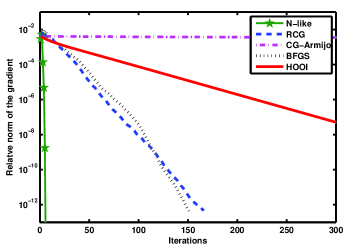
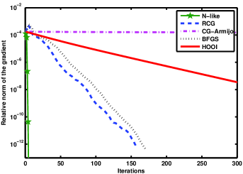
Fig. 1: Convergence for multilinear rank tensor approximation: number of iterations versus the relative norm of the gradient $\|\mathop{\operator@font grad}\nolimits_{\rho_{A}}(P^{n})\|/\rho_{A}(P^{n})$ at a logarithmic scale. Left: $100\times 100\times 100$ tensor approximated by a rank-$(5,5,5)$ tensor. Right: $100\times 150\times 200$ tensor approximated by a rank-$(15,10,5)$ tensor.

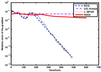
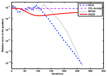
Fig. 2: Convergence for multilinear rank tensor approximation: number of iterations versus the relative norm of the gradient $\|\mathop{\operator@font grad}\nolimits_{\rho_{A}}(P^{n})\|/\rho_{A}(P^{n})$ at a logarithmic scale. Left: $200\times 200\times 200$ tensor approximated by a rank-$(10,10,10)$ tensor. Right: $50\times 50\times 50\times 50$ tensor approximated by a rank-$(5,5,5,5)$ tensor.

Fig. 1 shows convergence results for two large size tensors $100\times 100\times 100$ and $100\times 150\times 200$ approximated by rank-$(5,5,5)$ and rank-$(15,10,5)$ tensors, respectively. In Fig. 2 we plot the convergence behavior of the RCG method for the best rank-$(10,10,10)$ approximation of a $200\times 200\times 200$ tensor (left) and for the best rank-$(5,5,5,5)$ approximation of a $50\times 50\times 50\times 50$ tensor. Due to the limited memory space, we were not able to run the N-like and BFGS quasi-Newton algorithms for the example on the left. Yet it was still possible to run RCG, L-BFGS, CG-Armijo and HOOI.

In Table 1 we display the average CPU times necessary to compute a low rank best approximation for tensors of different sizes and orders by N-like, RCG, BFGS and L-BFGS quasi-Newton methods. We have performed 100 runs for each example.

Table 1: Average CPU Time

Tensor size and rank	N-like	RCG	BFGS	L-BFGS
$50\times 50\times 50,\;$ rank-$(7,8,5)$	2 s	6 s	24 s	13 s
$100\times 100\times 100,\;$ rank-$(5,5,5)$	70 s	75 s	150 s	94 s
$200\times 200\times 200,\;$ rank-$(5,5,5)$	-	11 min	-	14 min
$50\times 50\times 50\times 50,\;$ rank-$(5,5,5,5)$	-	9 min	11 min	-

Resume. First we mention that there is no guarantee that the N-like and RCG iterations converge to a local maximizer of the generalized Rayleigh-quotient. However, in the examples presented in Fig.1 and Fig.2 the limiting points are local maximizers. As the numerical experiments have shown, the N-like method has the advantage of fast convergence. Unfortunately, for large scale problems, the N-like algorithm can not be applied, as mentioned before. Even when it is possible to apply N-like algorithm, it needs a large amount of time per iteration. As an example, for the best rank-$(10,10,10)$ of a $180\times 180\times 180$ tensor, one N-like iteration took three minutes. Related algorithms which explicitly compute the Hessian and solve the Newton equation, such as [8, 18], and those which approximately solve the Newton equation such as the trust region method [17], face the same difficulty for large scale problems. On the other hand, the low cost iterations of the RCG method makes it a good candidate to solve large size problems. The convergence rate is comparative to that of the BFGS quasi-Newton method in [25], but at much lower computational costs. Our experiments exhibit the shortest CPU time for the RCG method. In the examples in which the tensor was a small perturbation of a low-rank tensor, the RCG algorithm exhibits quadratic convergence.

4.3.2 Subspace Clustering

The experimental setup consists in choosing $r$ subspaces in ${\mathbb{R}}^{3}$ ($r=2,3$ and $4$) and collections of $200$ randomly chosen points on each subspace. Then, the sample points are perturbed by adding zero-mean Gaussian noise with standard deviation varying from $0\%$ to $5\%$ in the different experiments. Now, the goal is to detect the exact subspaces or to approximate them as good as possible. For this purpose, we apply our N-like and RCG algorithms to solve the associated optimization task, cf. Section 3.1. The error between the exact subspaces and the estimated ones is measured as in [33], i.e.

$$\mathrm{err}:=\frac{1}{r}\sum\limits_{j=1}^{r}\mathrm{arccos}\biggl{(}\frac{1}{m_{j}^{2}}|\operatorname{tr}(P_{j}\tilde{P}_{j})|\biggr{)},$$ (111)

where $P_{j}$ is the orthogonal projector corresponding to the exact subspace and $\tilde{P}_{j}$ the orthogonal projector corresponding to the estimated one.

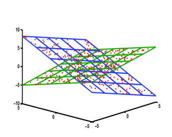
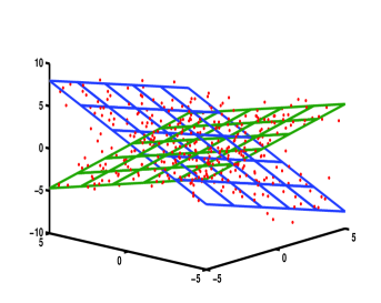
Fig. 3: Left: Data points drawn from the union of two subspaces of dimension $2$ (through the origin) of ${\mathbb{R}}^{3}$. Right: Data points from the left figure slightly perturbed by zero mean Gaussian noise with $5\%$ standard deviation.

It can be easily checked that in the case of unperturbed data there is a unique non-degenerate minimizer of $\rho_{A}$, and it yields the exact subspaces. Thus, we expect that for noisy data the global minimizer still gives a good approximation. Since $\rho_{A}$ has many local optima, for an arbitrary starting point our algorithms can converge to stationary points which lead to a significant error between the exact subspaces and their approximation. Thus, in what follows, we briefly describe a method (PDA, see below) for computing a suitable initial point which guarantees the convergence of our algorithms towards a good approximation of the exact subspaces in our numerical experiment:

The Polynomial Differential Algorithm (PDA) was proposed in [33]. It is a purely algebraic method for recovering a finite number of subspaces from a set of data points belonging to the union of these subspaces. From the data set finitely many homogeneous polynomials are computed such that their zero set coincides with the union of the sought subspaces. Then, an evaluation of their derivatives at given data points yields successively a basis of the orthogonal complement of subspaces one is interested in. For noisy data, a slightly modified version of PDA [33] yields an approximation of the unperturbed subspaces. This “first" approximation turned out to be a good starting point for our iterative algorithms which significantly improved the approximation quality.

For each noise level we perform 500 runs of the N-like and Local-CG algorithms for different data sets and compute the mean error between the exact subspaces and the computed approximations. As a preliminary step, we normalize all data points, such that no direction is favored.

In Fig. 3, $400$ randomly chosen data points which lie exactly in the union of two $2$-dimensional subspaces of ${\mathbb{R}}^{3}$ (left) and their perturbed images (right) are depicted. Moreover, the two plots display the exact subspaces (left) as well as the ones computed by our N-like algorithm (right). The error between the exact subspaces and our approximation is ca. $2^{\circ}$, whereas the error for the PDA approximation is ca. $5^{\circ}$.

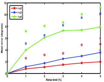
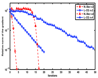
Fig. 4: Left: The mean error for noise levels from $0\%$ to $5\%$ and different number of subspaces. The disconnected symbols refer to the initial error (PDA) and the corresponding continuous lines refer to the error estimated by our algorithms. Right: Convergence of N-like and RCG for subspace clustering: number of iterations versus the relative norm of the gradient $\|\mathop{\operator@font grad}\nolimits_{\rho_{A}}(P^{n})\|/\rho_{A}(P^{n})$ at a logarithmic scale. Data points from $3$ and resp. $4$ subspaces perturbed with $5\%$ Gaussian noise. Average CPU time: ca. $0.4$ and ca. $2$ seconds for the N-like and RCG algorithm, respectively (1.8 GHz Intel Core 2 Duo processor).

In Fig. 4, we plot the mean error (left) for different noise levels and different number of subspaces. We have included also the mean error for the starting point of our algorithms, i.e. for the PDA approximation. On the right we demonstrate the fast convergence rate of the N-like and RCG algorithms for the case of $3$ and, respectively, $4$ subspaces.

Resume. Our numerical experiments have proven that (i) the minimization task proposed in Section 3 is capable to solve subspace detection problems and (ii) our numerical algorithms initialized with the PDA starting point yield an effective method for computing a reliable approximation of the perturbed subspaces. How the approximation of the perturbed subspaces varies when the noise in the data follows some law of distribution, is the subject of future investigation.

5 Appendix

Here we provide a proof of Proposition 2.3, which states that there exists a global Riemannian isometry $\varphi$ between $\mathrm{Gr}^{\otimes r}({\bf m},{\bf n})$ and $\mathrm{Gr}^{\times r}({\bf m},{\bf n}).$

Proof.

The surjectivity of $\varphi$ is clear from the definition of $\mathrm{Gr}^{\otimes r}({\bf m},{\bf n})$. To prove the injectivity of $\varphi$ we use induction over $r$. Choose $(P_{1},..,P_{r}),\;(Q_{1},\dots,Q_{r})\in\mathrm{Gr}^{\times r}({\bf m},{\bf n})$ such that $P_{1}\otimes\dots\otimes P_{r}=Q_{1}\otimes\dots\otimes Q_{r},$ i.e.

$$\alpha_{ij}P_{r}=\beta_{ij}Q_{r}\quad\textrm{for all}\;i,\;j,$$ (112)

where $\alpha_{ij}$ and $\beta_{ij}$ are the entries of $P_{1}\otimes\dots\otimes P_{r-1}$ and $Q_{1}\otimes\dots\otimes Q_{r-1}$, respectively.
Thus it exists $\gamma\in{\mathbb{C}}$ such that $P_{r}=\gamma Q_{r}$. Since $P_{r}$ and $Q_{r}$ have only $0$ and $1$ as eigenvalues it follows that $\gamma=1$ and $P_{r}=Q_{r}$. Therefore, $P_{1}\otimes\dots\otimes P_{r}=Q_{1}\otimes\dots\otimes Q_{r}$ implies that

$$P_{1}\otimes\dots\otimes P_{r-1}=Q_{1}\otimes\dots\otimes Q_{r-1}$$ (113)

and the procedure can be repeated until we obtain $P_{j}=Q_{j}$, for all $j=1,\dots,r$. Thus the injectivity of $\varphi$ is proven. So $\varphi$ is a continuous bijective map with continuous inverse $\varphi^{-1}$ due to the compactness of $\mathrm{Gr}^{\times r}({\bf m},{\bf n})$. Moreover, the map $\varphi$ is smooth since the components of $P_{1}\otimes\dots\otimes P_{r}$ are polynomial functions. Let $P:=(P_{1},\dots,P_{r})$ and ${\bf P}:=P_{1}\otimes\dots\otimes P_{r}$. Consider the tangent map of $\varphi$ at $P$, i.e.

$$\begin{array}[]{c}D\varphi(P):\mathrm{T}_{P}\mathrm{Gr}^{\times r}({\bf m},{\bf n})\rightarrow\mathrm{T}_{\bf P}\mathrm{Gr}^{\otimes r}({\bf m},{\bf n}),\\[5.69054pt] (\xi_{1},\dots,\xi_{r})\mapsto\displaystyle\sum\limits_{j=1}^{r}P_{1}\otimes\dots\otimes\xi_{j}\otimes\dots\otimes P_{r}.\end{array}$$ (114)

With the inner products (12) and (13) defined on $\mathfrak{her}_{N}$ and $\mathfrak{her}_{n_{1}}\times\cdots\times\mathfrak{her}_{n_{r}}$, respectively, one has

$$\left<D\varphi(P)\xi,D\varphi(P)\eta\right>=\displaystyle\sum\limits_{j=1}^{r}M_{j}\operatorname{tr}(\xi_{j}\eta_{j})=\langle\xi,\eta\rangle,\quad M_{j}:=\prod\limits_{k=1,\,k\neq j}^{r}m_{k}.$$ (115)

This implies that the tangent map $D\varphi(P)$ is a linear isometry. Thus, it is invertible and therefore $\varphi$ is a local diffeomorphism. Moreover, since $\varphi$ is bijective it is a global diffeomorphism, giving thus a global Riemannian isometry when the metric on $\mathrm{Gr}^{\times r}({\bf m},{\bf n})$ is defined by (15). ∎

References

• [1] P. A. Absil, R. Mahony, and R. Sepulchre, Optimization algorithms on matrix manifolds, Princeton University Press, 2007.
• [2] R. Bhatia, Partial traces and entropy inequalities, Linear Algebra and its Applications, 370, (2003), pp. 125–132.
• [3] R. W. Brockett, Least squares matching problems, Linear Algebra and its Applications, 122–124, (1989), pp. 761–777.
• [4] P. Comon, Tensor decompositions: State of the art and applications, Mathematics in Signal Processing, V, Oxford University Press, Oxford, (2002), pp. 1–24.
• [5] O. Curtef, G. Dirr and U. Helmke, Riemannian optimization on tensor products of Grassmann manifolds: Applications to generalized Rayleigh-quotients manifolds, arXiv:1005.4854, (2011).
• [6] G. Dirr, U. Helmke, M. Kleinsteuber and Th. Schulte-Herbrüggen, Relative C-numerical ranges for applications in quantum control and quantum information, Linear and Multilinear Algebra, 56, (2008), pp. 27–51.
• [7] C. Eckart, and G. Young, The approximation of one matrix by another of lower rank, Psychometrika, 1, (1936), pp. 211–263.
• [8] L. Elden, and B. Savas, A Newton-Grassmann method for computing the best multilinear rank-$(r_{1},r_{2},r_{3})$ approximation of a tensor, SIAM J. Matrix. Anal. Appl., 31(2), (2009), pp.  248–271.
• [9] D. Gabay, Minimizing a differentiable function over a differentiable manifold, Journal of Optimization Theory and Applications, 37(2), (1982), pp. 177–21.
• [10] K. A. Gallivan, A. Srivastava, X. Liu, and P. Van Dooren, Efficient algorithms for inferences on Grassmann manifolds, Proceedings of IEEE Conference on Statistical Signal Processing, (2003), pp. 315–318.
• [11] G. H. Golub, Matrix computations, Johns Hopkins University Press, Baltimore, Maryland, 3rd edition, 1996.
• [12] W. Greub, Multilinear algebra, Springer-Verlag , New York, 1978.
• [13] U. Helmke, K. Hüper and J. Trumf, Newton’s method on Grassmann manifolds, arXiv: 0709.2205v2, (2007).
• [14] U. Helmke and J. B. Moore, Optimization and dynamical systems, Springer-Verlag London, 1994.
• [15] M. W. Hirsch, Differential topology, Springer-Verlag, New York, 1976.
• [16] J. Ho, M. H. Yang, J. Lim, K. C. Lee and D. Kriegman, Clustering appearances of objects under varying illumination conditions, CVPR, (2003), pp. 11–18.
• [17] M. Ishteva, L. De Lathauwer, P. A. Absil, and S. Van Huffel, On the best low multilinear rank approximation of higher-order tensors, based on trust region scheme, Technical report: ESAT-SISTA-09-142, (2009).
• [18] M. Ishteva, L. De Lathauwer, P. A. Absil, and S. Van Huffel, Differential-geometric Newton method for the best rank-$(R_{1},R_{2},R_{3})$ approximation of tensors, Numerical Algorithms, 51(2), (2009), pp. 179–194. Tributes to Gene H. Golub Part II.
• [19] S. Lang, Algebra, Rev. 3rd ed., Graduate Texts in Mathematics, 211, Springer-Verlag, New York, 2002.
• [20] L. De Lathauwer, B. De Moor, and J. Vandewalle, A multilinear singular value decomposition, SIAM J. Matrix Anal. Appl., 21(4), (2000), pp.  1253–1278.
• [21] L. De Lathauwer, B. De Moor, and J. Vandewalle, On the best rank-$1$ and rank-$(R_{1},R_{2},\dots,R_{N})$ approximation of higher-order tensors, SIAM J. Matrix Anal. Appl., 21(4), 2000, pp. 1324–1342.
• [22] R. Mahony, U. Helmke, and J. B. Moore, Gradient algorithms for principal component analysis, J. Austral. Math. Soc. Ser., B37, (1996), pp. 430–450.
• [23] Nielsen and Chuang, Quantum computation and quantum information, Cambridge University Press, 2000.
• [24] J. Nocedal and S. J. Wright, Numerical optimization, Springer-Verlag New York, 2nd edition, 2006.
• [25] B. Savas, Algorithm package manual: Best low rank tensor approximation, Departament of Mathematics, Linköping University, Linköping, Sweden, (2008). (http://www.mai.liu.se/ besav/soft.html)
• [26] B. Savas, and L. -H. Lim, Quasi-Newton methods on Grassmannians and multilinear approximations of tensors, SIAM J. Sci. Comput., 32(6), (2010), pp. 3352–3393.
• [27] M. Shub, Some remarks on dynamical systems and numerical analysis, Dynamical systems and partial differential equations (Caracas), (1986), pp.  69–91.
• [28] V. De Silva, L. -H. Lim, Tensor rank and the ill-posedness of the best low-rank approximation problem, SIAM J. Matrix. Anal. Appl., 30(3), (2008), pp.  1084–1127.
• [29] T.  Smith, Optimization techniques on Riemannian manifolds, Fields Institute Communications, 3, (1994).
• [30] M.  Tipping and C. Bishop, Mixtures of probabilistic principal component analyzers, Neural Computation, 11(2), (1999).
• [31] L. R. Tucker, Some mathematical notes of three-mode factor analysis, Psychometrika, 31, (1966), pp. 279–311.
• [32] C.  Udriste, Convex functions and optimization methods on Riemannian manifolds, Kluwer Academic Publishers, Dordrecht, 1994.
• [33] R. Vidal, Y. Ma, and J. Piazzi, A new GPCA algorithm for clustering subspaces fitting, differentiating and dividing plynomials, CVPR, (2004).
• [34] T.  Wei, and P.  Goldbart, Geometric measure of entanglement and applications to bipartite and multipartite quantum states, Phys. Rev. A, 68(042307), (2003).