Proper motions of Local Group dwarf spheroidal galaxies I: First ground-based results for Fornax

Abstract

In this paper we present in detail the methodology and the first results of a ground-based program to determine the absolute proper motion of the Fornax dwarf spheroidal galaxy.

The proper motion was determined using bona-fide Fornax star members measured with respect to a fiducial at-rest background spectroscopically confirmed Quasar, QSO J0240-3434B (catalog ). Our homogeneous measurements, based on this one Quasar gives a value of ($\mu_{\alpha}\cos\delta$,$\mu_{\delta}$)$=(0.64\pm 0.08,-0.01\pm 0.11)$ mas y^-1. There are only two other (astrometric) determinations for the transverse motion of Fornax: one based on a combination of plates and HST data, and another (of higher internal precision) based on HST data. We show that our proper motion errors are similar to those derived from HST measurements on individual QSOs. We provide evidence that, as far as we can determine it, our motion is not affected by magnitude, color, or other potential systematic effects. Last epoch measurements and reductions are underway for other four Quasar fields of this galaxy, which, when combined, should yield proper motions with a weighted mean error of $\sim 50\,\mu$as y^-1, allowing us to place important constraints on the orbit of Fornax.

1 Introduction

The proper motions (PMs) of the satellites of the Milky Way (MW), when combined with existing radial velocities, allow us to determine the space velocity vectors of these satellites of our galaxy, which in turn place important constraints on their orbits (see, e.g., Besla et al. (2007), Piatek et al. (2007)). This knowledge is crucial to determine if these galaxies are gravitationally bound to the Galaxy, and to our understanding of the evolution and origin of its satellite system (Byrd et al. (1994)). The PMs of the satellites of the MW are necessary to understand: a) the origin of the MW satellite system and its relationship with the formation and evolution of the galactic halo (Dinescu et al. (2000), Palma et al. (2002), Carlin et al. (2009)), b) the nature and origin of the streams that seem to align different subgroups of these galaxies (Lynden-Bell (1982), Lynden-Bell and Lynden-Bell (1995), Piatek et al. (2005)), and c) the role of tidal interactions in the evolution and star formation history of low mass galaxies (Zaritsky and Harris (2004), Piatek et al. (2005), Noël et al. (2009), Mayer (2010)). A comprehensive study of the MW’s satellite system can lead to a greater general understanding of galaxy evolution and the physical processes governing star formation in galaxies.

From another perspective, reliable space motions of Local Group galaxies is a key ingredient to populate the phase-space components for flow models which predict the dynamical evolution of the local universe. Indeed, current center-of-mass locations and motions from the present distribution of galaxies can be used as boundary conditions to “trace them back in time” (Peebles, 1989, 1994) and to test the paradigm that galaxy clusters grew by gravitational instabilities from an originally smoother medium, with small random motions. These earlier simulations have not been repeated too often due to the growing realization that more complex effects such as tides, satellite interactions, accretion and mergers, influencing the growth of galaxies with time (specially at epochs earlier than 7-8 Gyr from now), can greatly complicate this approach. Nevertheless, the motions of local group galaxies can be used as boundary conditions in a first aproximation to carry out the above analysis. This goal has become one of the important drivers behind future astrometric space missions, such as SIM (Unwin et al. (2008), specially their Figure 13), which expect to measure PM for Local Group galaxies with a precision ten times better than what can be achieved with present techniques.

With the above motivations in mind, in the year 2000 we started a ground-based program aimed at determining, the absolute PM of three southern dwarf Spheroidal (dSph) galaxies, Carina, Fornax, and Sculptor, with respect to known background Quasars (QSOs) that can be used as inertial reference points. Three epochs, over a period of eight years were obtained using a single telescope+detector set up: Ours is then the first entirely optical CCD/ground-based proper motion study of an external galaxy other than the Magellanic Clouds.

In this paper we report on the first results from this program, based on one QSO field in Fornax, for which we have data of good enough quality to allow us to asses the expected precision of our measurements, and to describe our methodology in detail. Last epoch measurements and reductions are underway for other four Quasar fields of Fornax, as well as for a similar number of QSO fields in Carina and Sculptor. The results for these will be presented in forthcoming papers.

In section 2 we describe our observational material and data acquisition strategies, in section 3 we describe our methodology for deriving the PMs, in section 4 we present the analysis for our QSO field, and in section 5 we present our main conclusions as well as a comparison to other results.

2 Observational material

All our observations were carried out with the “Super Seeing Imager”, SuSI2, attached to one of the Nasmyth focii of the ESO 3.5 m NTT telescope at La Silla Observatory. The overall characteristics of the detector, a mosaic of two EEV 44-82, 2k$\times$4k, 15 $\mu$m pixel, thinned, anti-reflection coated chips covering a field-of-view (FOV) of 5.5$\times$5.5 arcmin², is fully described in D’Odorico (1998) and D’Odorico et al. (1998). The measured charge transfer efficiency, CTE (serial and parallel readouts) is better than 1 part in $10^{6}$, while both chips have been found to be linear within $\pm$0.15% over the full range 0-60,000 ADUs. All our measurements are based on objects within this linearity range. On the other hand, CTE is considered to be have a negligible impact on our astrometric measurements, as the sky background (unlike the case of the space-based, e.g., HST, data) is quite large, typically between 300 and 900 ADUs (in comparison to the few counts on the HST cameras): Higher background signals fills-in charge traps on the detector, leaving no empty traps to be filled by signal from a source (for details see, e.g., Bristow et al. (2006), specially his Figure 10).

In the un-binned mode, in which all our data was acquired, we have adopted for the plate scale the value given in the SuSI2 manual of $0.0805\pm 0.0002$ arcsec pix^-1. We have verified the accuracy of this value, following the procedure described in Costa et al. (2009), through the use of the IRAF routines ccxymatch, ccmap and cctran on an astrometric field in the periphery of the $\Omega$Cen cluster (van Leeuwen et al., 2000), with plenty of stars in the FOV. All the astrometric and refraction-series frames (see section 4) were acquired through a “Bessel R #813” filter, whereas blue frames needed for constructing color-magnitude diagrams (CMDs) used the “Bessel B #811” filter. Both filters are part of the standard set for the instrument.

The QSO field analyzed here is that of the double QSO J0240-3434, located at $(RA,DEC)=(02:40:07.7,-34:34:20)$ (position for the A component, although for reasons that are explained later one we used only the B-component for our PM, see section 3.2). Exposure times for the science frames varied between 250 s and 900 s (see Table 1). At the start of our program we adjusted the exposure time on the basis of the ambient seeing, later it was decided to use a fixed exposure (900 s) in all cases.

Because our measurements involve the displacement of Fornax stars relative to a fixed point (the QSO in the FOV), we used only one of the two chips of the array, Chip #46, which has a slightly better read-out noise (4.6 e^-/pix, with a gain of 2.26 e^-/ADU), and better overall cosmetics than its twin. Given the alt-az nature of the telescope, and the Nasmyth location of the instrument, a rotator-adaptor allows one to select the orientation of the detector on the sky, and keeps it fixed during the observations. All our observations were acquired with a nominal rotation angle of zero degrees: In this orientation North increases in the Y-pixel direction, while East increases in the X-pixel direction (for more details see section 3.1).

For reasons that will be become apparent later on, all observations were acquired by placing the QSO at a nominal pixel position of $(x,y)=(3\,000,\,2\,100)$ near the middle of chip #46. Given the extraordinary pointing accuracy of the telescope, this meant that all our frames are centered at this position $\pm$ few pix (few=$\leq 7$ pix $\sim 0.6$ arcsec). This procedure was greatly simplified by the use of the so-called “Observing Blocks” that determine the way in which a set of observations with a given telescope+instrument is to be carried out, a common feature of the data acquisition software at all ESO facilities (other relevant factors such as hour angle, airmass, and the range of acceptable seeing and sky transparency conditions were however decided by the observer).

For calibration purposes at least five dome illumination flats in the B and R filters were secured every night. Some sky illumination flats were also acquired to check our basic calibrations (see below), pointing the telescope one hour to the East/West (sunset/dawn) of the meridian, and at a declination equal to the latitude of the observatory, always with the telescope tracking, and applying small offsets in between exposures to facilitate the elimination of any possible stellar images during the combination of the images. Also, at least twenty zero exposure time bias frames were obtained every night. Given the negligible dark current of the instrument, no dark frames were acquired. The mosaic data was split into the two individual chips, and only data from chip #46 was used subsequently. All frames (from now on single-chip #46 exclusively) were calibrated, on a night-by-night basis, using standard IRAF routines within the noao.imred.ccdred package for combining the zero & flats frames, and applying them to the science images. In particular, zero and illumination flat frames were median-combined with an iterative ”avsigclip” algorithm with an upper & lower sigma clipping of 2.5. For combination, the flats were scaled using their respective median values computed from a region free from cosmetic defects in the middle of the chip, encompassing 1300$\times$3500 pix² (no scaling was used for the zero exposure frames, as their level remained constant, save by Poisson noise fluctuations).

An overscan region, resulting from the average of 38 non-exposed columns to the right of chip #46, was fitted with three pieces of a third degree spline function, which was subsequently subtracted from all frames. This function provided a smooth and well sampled fit to the observed overscan all the way to the usable edges of the chip: Starting from a full exposed CCD area 2048$\times$4096 pix² (each chip has in total 2144$\times$4096 pix²), the final trimmed images have 2026$\times$4086 pix², where rapidly variable illumination and/or CCD boundary defects were excluded altogether.

Whenever we had a reasonable number of well-exposed sky flats (at least three), the science data was reduced with sky and dome flats independently to asses any large remaining gradients that may be induced by a non-uniform illumination from the dome flat screen. These tests indicated that, after flat-fielding, there remained low-frequency trends across the chip using either dome or sky flats, and that sky flats were not always necessarily better than dome flats, perhaps as a consequence of scattered light coming into the detector from the telescope structure (through its wind vents) at sunset/dawn. Larger trend were noticed in our earlier epoch data. Over the years a number of improvements were made to the telescope baffling, which alleviated these problems in the later epoch frames, as indeed observed in our data. In any case, the maximum background gradient found in these comparisons was 10% accross the entire chip (although typically it was $\sim$5% or smaller), and we did not find any large gradients on scales smaller than a few hundred pixels. Therefore, locally, at any location on the chip, the sky could be considered essentially constant. Since our primary concern is astrometry, and not photometry, we opted for reducing all our data (i.e., B and R-band frames) consistently using dome flats only.

After the basic calibrations described above were performed for the data from all epochs, each frame was used independently to determine $(x,y)$ positions and photometry for a carefully selected subset of objects in the FOV, thus starting the astrometric reduction steps described in detail in the following section.

3 Astrometric reduction steps

The basic reduction steps are similar to those described in Costa et al. (2009) in the context of the so-called “QSO method” in which the relative displacement of a fiducial at-rest point (the QSO) is measured with respect to a set of bona-fide Fornax stars, registered to a common reference system. In what follows we give further details on either departures from the basic astrometric steps described by Costa et al. (2009), or provide more detailed explanations whenever required.

After grouping all (astrometric) data for a given QSO field, we created a catalog of all observations with basic bookkeeping information such as date of observation, exposure time, hour angle, airmass, etc., of the images. We then examined all images to determine their overall quality, including average seeing ($FWHM$), sky background ($<sky>$), and sky noise ($\sigma_{\mbox{sky}}$), information which was cross-correlated with the night sky conditions as recorded on the various observatory logs and by the DIMM seeing associated to each image as recorded on the ESO Science Archive. This first quality control allowed us to discard unusable images (e.g., trailed or badly elongated images, very low counts due to variable sky transparency, and “bad” ($>1.2$ arcsec seeing)). In Table 1 we summarize the observational material used throughout this work. The meaning of the various entries will be explained in the following subsections.

3.1 Building the initial astrometric reference system & deriving pixel coordinates

From the basic data set obtained as above, we selected a set of good-seeing ($FWHM<0.7$ arc-sec), near meridian, consecutive frames to create the so-called “Standard Frame of Reference” (SFR, which will be used later on in the astrometric registration process), and selected one of them as a “master” frame (see Table 1). From this master frame we created a list of “good” reference stellar images to define our initial “local reference system” (“LRS” from now on). To create the LRS we used the DAOPHOT tasks implented in the IRAF package under noao.digiphot.daophot. We start by running the daofind task with a small threshold of 4$\times\sigma_{\mbox{sky}}$, to have as many detections as possible (it is important to start with a low threshold, since it allows us to use these hits to eliminate potential nearby companions to much brighter good reference stars, see below). Proper care was taken to edit relevant image parameters such as the mean FWHM of the stellar images, $\sigma_{\mbox{sky}}$, the minimum and maximum good data value (taken as $<sky>-10\times\sigma_{\mbox{sky}}$ and 60,000 ADUs respectively). The output of daofind had, at this stage 8,235 hits, in total.

We note that the orientation of the master frame with respect to the Celestial RA, DEC coordinate system defines also the orientation of our PMs with respect to $\mu_{\alpha}\cos\delta$ and $\mu_{\delta}$ since both the individual SFR frames and all of the other astrometric frames are eventually transformed into the master frame (see section 3.4). Therefore, it is important to ascertain any local “rotation” of our $(x,y)$ coordinates with respect to $(\alpha,\delta)$. This was done following the same procedure described in Costa et al. (2009): We found a negligible rotation of our master frame ($359.545\pm 0.018$ deg), and therefore no further correction (which go as the cosine and sine of the above angle) was applied to our PMs. Since the NTT is an Alt-AZ telescope, and the instrument is mounted on one of the Nasmyth focii, we were concerned that the adaptor-rotator could have introduced significant rotations between succesive frames due to mechanical innacuracies in the positioning of the rotator. When explicitely solving for this remaining rotator-induced rotation we found that they were all very small (the largest measured rotation was 0.017 deg, although it was typically 0.0001 deg). In any case, we note that our registration procedure (in particular the first-order cross terms) would fully account for this effect when comparing the SFR to all other individual astrometric frames.

Photometry with the task phot was then performed using the input list described above on this particular master frame, and using a rather large aperture of 15 pix (1.2 arcsec). To determine the local sky, an annulus of width 5 pix and inner radius of 20 pix was adopted. An iterative sigma-clipping algorithm with upper & lower rejection limit of 2.5, as well as an upper & lower clipping factor of 10% percent, was adopted to robustly determine the mean local value of the sky around each object, as measured from the modal value (recommended for crowded fields). The output of the phot task was then used to make a preliminary semi-automatic “cleaning” of the sample by eliminating objects, using the pexamine tool (given the larger number of hits, at this stage we departed from the Costa et al. (2009) procedure of examining the possible LRS stars by eye, which we did only at a later time). Objects were deleted either because they were too close to the frame boundaries (and thus could become missing in slightly offset frames from other epochs), or because they were at or near a set of two bad columns in the upper part of the chip. Additionally, image shape or photometric parameters reported by the daofind and phot tasks, such as “sharpness”, “roundness”, and magnitude error were used as a preliminary guide to select a set of well measured star images on the master frame. Spurious detections around bright stars, as well as multiple hits on extended objects were also eliminated based on an eye inspection of the daofind hits on the master frame. At this stage the number of detections dropped to some 952 objects. We then ran a code to eliminate, out of this latest sample, any object that had a companion in the original daofind output, closer than a certain radius, in this case, 20 pix, rendering the number of objects down to 422. The choice of this radius is somewhat arbitrary and is a compromise between a large enough number of LRS stars (i.e., choosing a small radius), and a set of well isolated stellar images for an astrometrically stable LRS (free from the influence of nearby/partially blended images, i.e., large radius), which is a function of the stellar density of the particular image. We note for example that when increasing this radius to 30 pix the number of objects dropped to 79 stars, which we considered insufficient given the further cleansing applied to the LRS (see below).

A small complication arose in the selection of the LRS stars since the Fornax Globular Cluster “4” at RA=02:40:07.70, DEC=-34:32:09.8, first described by Hodge (1961) was present in the images in the North section of the chip. The cluster was not well resolved in the images, leading to a large number of stars with nearby companions in a crowded field. To avoid potential astrometric problems with these stars, a reasonable region around the cluster was removed. In the end, this step did not have an important impact on the x-y distribution of our reference stars (see Figure 15).

With this list we then interactively ran the tasks pstselect and psf and selected a subset of high S/N stars well distributed over the entire chip, to build a point spread function (PSF) for the master image. We let DAOPHOT decide what psf function to adopt, based on the best $\chi^{2}$ of the fit, as reported by IRAF, on account of the differing seeing/distortions in different frames. Given the large number of stars available, we also let the PSF to vary accross the chip (fitting the lookup parameters to each individual image), by adopting varorder=3 within the daopars parameter set which is used to drive the psf task. One advantage of running these taks interactively is that stars with previously unseen companions or with cosmic rays and/or hot pixels can be excluded in the construction of the psf (stars with previously undetected close companions or affected by hot pixels were also excluded from the LRS list from which the psf list was built, but not the ones affected by cosmic-rays, which are image-dependent). As an example, for the master frame, out of 200 initially selected PSF stars, only 170 survived this interactive cleaning, and were used to create the PSF.

Once a PSF for the master frame was created, the iterative PSF-fitting DAOPHOT task peak was used to compute final $(x,y)$ coordinates for all the LRS stars. Two further cleaning steps of the initial LRS were performed at this stage. First, from the peak output (which, on account of using a PSF built from the image itself, provides a much refined measurement of image parameters than daofind and phot do), objects with large magnitude errors ($\sigma_{\mbox{mag}}>0.1$ mag), and/or with an unusually large number of iterations (in comparison with the bulk of objects) to converge to the solution were deleted. Finally, this latter list was applied to the worst FWHM astrometric image of this QSO field to create a PSF and to run peak, again deleting objects that, on this relatively lesser quality image, had parameters similar to those used to eliminate objects in the (good quality) master frame. At this stage we had built a sample of 260 well measured stars over the entire FOV of the chip which became our initial LRS for the entire set of frames. The approximate magnitude and color range for the LRS is $17.0\leq R\leq 21.2$ and $0.0\leq B-R\leq 2.0$ (see Section 4).

Once the initial LRS was built, we succesively created PSFs for all frames, always in interactive mode to eliminate stars affected by cosmic-rays (therefore number of PSF stars was variable, between a minimum of 128 and a maximum of 178 stars), and used them to compute $(x,y)$ coordinates for all the LRS stars and the QSO on each frame using the task peak. This was perhaps the most time-consuming part of the whole process, given its interactive nature, and that for each frame the psf task had to compute the goodness-of-fit for the six functions available within DAOPHOT: Gaussian, two Moffat functions, two Penny functions, and one Lorentzian). For each frame we kept the radius of PSF model fixed at 14 pix, whereas the fitting radius was adjusted to $1.2\times FWHM$ of the corresponding frame, with a maximum value equal to the adopted PSF model radius. The ouput of the peak routine are the raw pixel coordinates of the LRS stars on each frame, which provide the basic ingredient for the subsequent astrometric reduction steps, described in the following subsections.

3.2 Precision of the pixel coordinates

Numerous tests were performed to determine the best precision attainable for our raw pixel coordinates as a function of the various PSF fitting parameters. First, given the degree of arbitrariness with which one includes or excludes PSF stars on each frame, we tested the sensitivity of our derived pixel coordinates to the exact nature of the stars chosen to build the PSF (ideally, one would like to have the same basic set of PSF stars for all frames, but the appearance of comsic rays - different on each image - on otherwise good PSF stars dot not allow this). In general, for all our frames, we started with the maximum number of stars (200) allowed by the psf task, and interactively deleted bad PSF stars, as explained before, but without regard of their S/N. The main motivation for this, besides the large number of suitable stars available, is to have a well sampled PSF over the entire FOV. Using one of the best FWHM consecutive frames indicated as “CTB-1” in Table 1, we computed a PSF (from 135 stars) and $(x,y)$ peak-based coordinates for a total sample of 1,200 stars, covering a wide magnitude range, and going actually $\sim$2 mag fainter than our LRS (equivalent to $\sim$1 mag brighter than the 4$\sigma_{\mbox{sky}}$ daofind detection limit for this frame), using our standard procedure: For these frames, this meant that the faintest PSF stars had a peak value above sky of $\sim 900$ counts (equivalent to an overall S/N over the whole image of $\sim 200$ on an aperture radius of $2\times FWHM$). We then computed another PSF but this time based only on stars with peak counts above $\sim 2000$ (in total the brightest 49 stars of the sample used to created the previous PSF), following the arguments proposed by Anderson et al. (2006) (see, in particular, their Section 3.5), and used this PSF to get $(x,y)$ coordinates for the same 1,200 stars. A comparion of the coordinates between the two sets indicate minuscule offsets of $<\Delta X>=(0.03\pm 0.84)\times 10^{-3}$ pix, and $<\Delta Y>=(-0.03\pm 1.0)\times 10^{-3}$ pix. The offsets do not show any trend vs. position, magnitude, or color of the stars. As we shall see later on, these offsets are a factor of 600 smaller than our (single measurement) centering accuracy when comparing consecutive frames (in time), and we therefore conclude that our choice of PSF stars is not biasing our pixel coordinates in any measurable way.

In our standard procedure we allow the software to decide (based on a $\chi^{2}$ test) what functional form for the PSF to adopt (in the case of frame CTB-1 this was a “penny2”, with 6 lookup tables), and we decided to also estimate the impact of this choice in our coordinates. For this purpose we fixed the PSF to the various functional forms allowed by the daophot task, but always using the same PSF stars and PSF parameters. The worst-case scenario was found when comparing the $(x,y)$ coordinates to those derived from a “gaussian” PSF with no spatial variation accross the chip. In this case, while no obvious positional trends are found (Figure 1), a magnitude dependent systematic trend (beyond the obvious increase in the scatter at fainter magnitudes) is clearly visible, (Figure 2) amounting to $(4.67\pm 0.61)\times 10^{-3}$ pix mag^-1. This trend disappears for any other PSF functional form. Even, with the next degree of freedom, i.e., a simple Gaussian PSF with only one lookup table (and no positional variation of the PSF accros the chip), we find a slope (in the X-coordinate) of $(-2.9\pm 2.4)\times 10^{-4}$ pix mag^-1, i.e., consistent with zero. We conclude that the trend is due to the inadequacy of a simple analytical PSF to model the actual PSF in the image, but that our exact choice of the PSF is irrelevant, as long as at least one lookup table of corrections is provided. In the end, for most of our frames, the automatic selection implied the use of either a “penny” or a ”moffat” function, and in this case our tests indicate that the choice of one or another yields offsets smaller than $5\times 10^{-3}$ pix, again smaller than the “repeatability” of our measurements (see below), and therefore it is of no concern.

Besides the actual PSF function adopted, there are various other parameters that control the way in which the PSF is used to determine centroids on the image, e.g., the width and radius of the sky annulus, the radius over which the of psf model is constructed, the actual PSF fitting radius used to determine centroids. Our tests indicate that, of all these parameters, it is the latter that has the most important relative influence on the derived centroids. In Figure 3 we show the rms scatter of coordinates from the same frame, CTB-1, as determined by the same (automatic) PSF model as a funtion of the adopted fitting radius. For this frame, with a seeing of 0.5 arcsec, the usually recommended value for crowded field photometry (Massey and Davies, 1992) equal to the FWHM (=6.5 pix) has of course an rms with respect to itself of zero. The upper curves are for the entire sample of stars, while the lower curves are for the brighter portion of the sample (more representative of the LRS stars). The smooth behavior of the (lower) curves in Figure 3 allows us to infer that the exact value of the adopted PSF fitting radius does not have an important impact on the stability of the derived coordinates but, of course, being a comparison of the coordinates derived from the same frame, it does not tell us about the optimum PSF fitting radius to use.

To actually estimate our centering accuracy, and the best PSF fitting parameters to use, we compared the coordinates derived from a pair of the best FWHM consecutive frames, CTB-1 and CTB-2 in Table 1. After determining an independent PSF for each frame (but using the very same PSF stars and PSF parameters for both frames), we computed $(x,y)$ coordinates for all our stars, and computed the rms of the pair of coordinates as derived from these two frames, as a function of the PSF fitting radius. Of course, the expectation is that best fitting radius should yield the smallest scatter on our coordinates. A small complication arose (see next paragraph) in that we had to register the coordinates, which introduced an additional source of noise (which, however, does not affect these conclusions): Once we had determined an optimal registration, the parameters from this unique transformation was used for the coordinates derived from all pairs. As it can be seen from Figure 4, a value for the fitting radius slightly larger than the FWHM of the image should be preferred. For both sets of curves in Figure 4, the rms decreases by about 5% when increasing the PSF fitting radius from the (nominal) FWHM to 1.5$\times$FWHM. Of course, when augmenting the fitting radius one runs into the increased risk that the centroids become more susceptible to possible faint nearby objects. For this reason, and as a compromise value, throughout this work we adopted a PSF fitting radius always equal to 1.2$\times$FWHM. Another important point from Figure 4 is the decrease of almost a factor of two in the registration residuals when going from a linear to a full quadratic registration polinomial (this is further explored in Section 4, see also Figure 13). Finally, the behavior and significance of the linear terms, which would address the commonality of the $(X,Y)$ pixel scales, is also presented in Section 4.

As it is clear from the discussion in the previous paragraph, and also from Figure 4, our estimates of the unit weight measurement error in the centroids is somewhat dependent on how well determined is the registration between the frames we are comparing. To study this particular point, we computed the rms of the coordinates by using various schemes of transformation equations. The most relevant conclusions from these tests is that the geometric transformation equations (registration) derived from data sets with different (faint) mag cuts (and with correspondingly different overall rms in the transformation itself), do not have an important impact in the derived $\sigma_{\mbox{X,Y}}$ vs. magnitude (see Figure 5). This means that the rms of the coordinates represents their intrinsic centering scatter, and not the effect of uncertainties in the registration itself. From this we conclude that, e.g., for “well measured” stars with $R<20.7$ (i.e., similar to the mag cut adopted for our LRS stars) the rms of the pixel differences is about 0.025 pix, or 0.018 pix ($\sim 1.5$ mas) pix for a single measurement, per coordinate. We also note that the sufficiently large number of stars with this magnitude cut ensures a good X-Y distribution over the entire FOV of the detector to map out the geometric distortions. We finally note the apparent ”break” of rapidly increasing scatter for $R>20.8$. As it can be appreciated from Figure 6, this is when, roughly, the source noise becomes comparable to the sky noise: In general, both throughout this work as well as in previous works from our group (e.g., Costa et al. (2009)) we adopt the magnitude for which $S/N>200$ as a guide for the faint cut of the LRS stars.

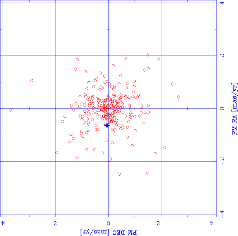
Figure 9: Vector point diagram based on all the initial 260 LRS stars. The dot with error bars represent the QSO.

After having obtained the raw pixel coordinates, the subsequent steps, all the way to obtaining PMs, follows very closely the procedure described by Costa et al. (2009), and includes computing LRS barycentric coordinates for each frame, computing the differential chromatic constants in this barycentric system (see next paragraph) for each LRS star and the QSO (using a series of frames taken specifically for this purpose (see Table 1)), and using these constants to correct the coordinates, registering all the LRS barycentric DCR-corrected coordinates onto a unique astrometric reference system (the SFR), and finally computing PMs for all LRS stars and the QSO through a simple linear fit of the barycentric DCR-corrected & registered coordinates vs. epoch such that, in the end, what we really measure is the reflex motion of the QSO relative to the bulk motion of star field (see Figure 9), by changing the signs we obtain the motion of the bona-fide Fornax stars with respect to the QSO, which thus defines the zero point of the astrometric system). In the following subsections we described in more detail than that given by Costa et al. (2009) some aspects of these reduction steps.

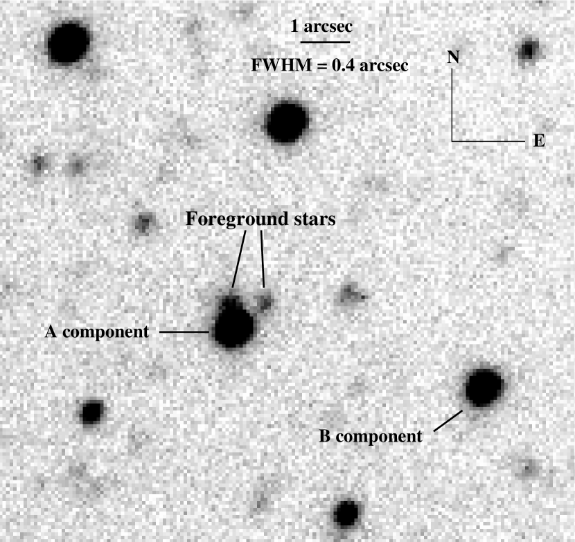
Figure 7: Best quality image (frame acquired on 2000-08-08, see Table 1) with a FWHM=0.4 arcsec, indicating the position of the A and B components of field QSO J0240-3434. The A component has two nearby foreground stellar companions (possibly members of Fornax). These stellar images blend with component A in the lesser quality frames of other epochs, deteriorating the astrometry. Only the SE (B) component was used throughout this work. Image size is $\sim$12 arc-sec on a side, and the image scaling is linear in ADUs. Several other foreground Fornax stars appear in the FOV.

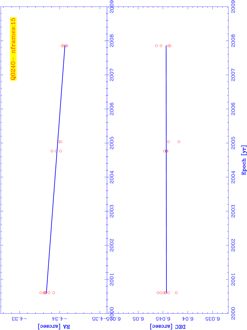
Figure 12: Barycentric position (DCR-corrected) vs. epoch diagram for QSO J0240-3434B. The slope is the PM of the QSO with respect to the LRS stars described in the text. The 15 frames indicated in Table 1 with $|HA|<1.5$ hrs went into this solution. The overall rms of the position vs. epoch fits are (0.88,1.27) mas in RA & DEC respectively.

We note that the field analyzed here actually contains two images of the same QSO J0240-3434, which is a known gravitational lens system (Tinney, 1995). Indeed one of the motivations to carry out this analysis in this particular was field was that we could have two independent measurements (using both images of the QSO) to assess our final positional and PM precision. However, this attempt was frustrated because one of the images (the NW image, component A), happened to have a nearby (foreground) companion star (presumably a member of Fornax), as shown in Figure 7. The companion was nearly resolved in the best images available, but was hidden in the lesser quality frames. Preliminary PM solutions using component A turned out to be unstable (e.g., strongly dependent on the image quality of the frames adopted in the solution), and with a large scatter in the position vs. epoch diagram (the equivalent of Figure 12). For this reason, these preliminary reductions were discarded altogether, and image A was not used at all in our astrometric solution. Therefore, all our results on this paper are based exclusively on component B of QSO J0240-3434.

3.3 Pixel coordinates pre-corrections

At this stage we are in a position to pre-correct our coordinates from any known effect altering their true focal-plane position. Of course, the first step would be to correct the coordinates from any known optical distortions in the system. Unfortunately, no dedicated study is available in the literature for the optical distortions on SuSI2 (as is the case of SOFI, another Nasmyth instrument at the NTT , and even this only deals with linear terms), nor could we, in the allocated time, to obtain images of a suitable astrometric calibration field to carry out such a study. We therefore do not apply any pre-correction to our raw coordinates at this stage, and deal with the effects of optical distortions through a (polynomial) registration to be applied later on. We note that, as long as the distortions are stable in time, by placing all targets at nearly the same location on the CCD, it is the derivatives of the distortions that matter, and these are likely to be very small (although not negligible, see Section 4).

The next relevant pre-correction to our coordinates comes from atmospheric refraction. For this we followed the prescription given by Stone (1996) with some modifications described in what follows. First, we implemented an iterative procedure to get true values starting from observed values, since atmospheric refraction is formulated in terms of true values (not knwon a priori). More specifically, we know that the relationship between the observed zenith distance ($z^{\prime}$) and the true one ($z$, not affected by refraction) is given by (see e.g., Equations (5.5) and (5.7) in Taff (1991)):

$$z-z^{\prime}=R_{m}(z)$$ (1)

where $R_{m}(z)$ is the refraction constant evaluated at the true zenith distance $z$ (see Stone (1996)). Since the correction to $z$ is small for the zenith distances considered in this work ($z^{\prime}<50^{o}$), our procedure starts by assuming that on the right-hand-side of Equation (1) we can approximate $z\sim z^{\prime}$ which allows us to compute (an approximate) $R_{m}(z)$, which then gives us $z$. By successive iterations, we rapidly (three to four iterations) converge into $z$ (and $R_{m}(z)$).

The computation of the index of refraction, related to $R_{m}(z)$ (see Equations 4 and 5 on Stone (1996)) requires knowledge of the atmospheric temperature, pressure, and relative humidity at the instant of data acquisition and the bandpass of the observations. All these parameters are available on the image headers, and are read from the observatory’s weather station. Latitude ($-29^{0}15^{\prime}18.4^{\prime\prime}$), and altitude (2,375 m above sea level) for the observatory were adopted from the observatory’s web page. Other relevant parameters (observed RA & DEC, LST) were also read from the image headers. For the calculation of the index of refraction (see Equations 14 to 17 in Stone (1996)), we adopted the central wavelength of the R-band filter, $6415.8\,\AA$, as given on the filter-page for SuSI2. With all this information, the raw pixel coordinates were corrected for refraction adopting the relevant ambient parameters for each individual frame.

So far, in the previous step, we have evaluated the refraction constant at one particular wavelength. However, the refraction constant $R_{m}(z)$ actually depends on the spectral energy distribution of the star being observed (see e.g., Equation (22) in Stone (1996)). Because on our LRS we have stars of different spectral types, as well as the QSO, the refraction constant will actually differ for all of them. This gives rise to a “differential displacement” of star positions, depending on their spectral energy distribution, which is a function of $z$ (see Equation (1)), known as Differential Chromatic Refraction (DCR). By contrast, the refraction correction described in the previous section affects all stars equally, regardless of their spectral type, and could be thus called “continuous refraction” to differentiate it from DCR. To correct our coordinates from DCR effects we followed the procedure indicated in Costa et al. (2009) (Section 3.4), for which we give a more detailed justification here. We must emphasize that these corrections are differential in the strict sense that they are computed with respect to the mean of the current LRS. More specifically, the computed barycentric coordinate, e.g., in the X-direction, for star “$i$”, $X^{\prime}_{i_{b}}$, is given by:

$$X^{\prime}_{i_{b}}=X^{\prime}_{i}-\frac{\sum_{j=1}^{N}X^{\prime}_{j}}{N}$$ (2)

where $X^{\prime}_{i}$ are the pixel coordinates measured on the detector, and $N$ is the (current) number of LRS stars that define the (current) barycenter. The primed pixel coordinates, being measured directly, are of course affected by atmospheric refraction. The relationship between the refraction-free coordinates $X_{i}$ (assumed to be oriented in the direction of RA), and the ones affected by refraction can be computed from Equation 1, and is given by Equation (29) on Stone (1996), which we include here for completeness:

$$X^{\prime}_{i}-X_{i}=R_{X_{i}}\times\sin\eta^{\prime}$$ (3)

where $R_{X_{i}}$ is the refraction constant for star $i$,

and $\eta^{\prime}$ is the so-called “angle of the star” (or parallactic angle) given by Equations (3) and (4) in Costa et al. (2009), which is itself a function of $z^{\prime}$ and the observed hour angle $H^{\prime}$. Equation (3) clearly shows that, due to atmospheric refraction, $X^{\prime}_{i}$ is a function of $z^{\prime}$ and $H^{\prime}$, i.e., one can write $X^{\prime}_{i}=X^{\prime}_{i}(z^{\prime},H^{\prime})$.

Replacing $X^{\prime}_{i}$ from Equation (3) into Equation (2), after some elementary algebra, we can see that, for the barycentric coordinates, it is valid that:

$$X^{\prime}_{i_{b}}(z^{\prime},H^{\prime})=X_{i,b}+\left(R_{X_{i}}\times\sin\eta^{\prime}-\frac{\sum_{j=1}^{N}R_{X_{j}}\times\sin\eta^{\prime}}{N}\right)$$ (4)

where, $X_{i,b}$ is the barycentric coordinate free from refraction ($\equiv X_{i}-\frac{\sum_{j=1}^{N}X_{j}}{N}$). In principle, the value of $\eta^{\prime}$ inside the summation on the right hand side of Equation (4) should be computed for the exact position of (each) star $j$ in the LRS. However, given our small FOV, this quantity can be considered constant, and therefore, Equation (4) can be re-written as:

$$X^{\prime}_{i_{b}}(z^{\prime},H^{\prime})=X_{i,b}+\left(R_{X_{i}}-\frac{\sum_{j=1}^{N}R_{X_{j}}}{N}\right)\times\sin\eta^{\prime}\equiv X_{i,b}+R^{DCR}_{X_{i}}\times\sin\eta^{\prime}$$ (5)

Where we have re-defined the (classical) refraction constant to a new DCR constant given by $R^{DCR}_{X_{i}}\equiv R_{X_{i}}-\frac{\sum_{j=1}^{N}}{N}$. Equation (5) reveals the true nature of the DCR correction, $R^{DCR}_{X_{i}}$ is nothing but a refraction constant for each LRS object with respect to the mean of the refraction constants for the (current) LRS, hence its name “differential”. A completely equivalent equation can be written for the Y ($\sim$DEC)-coordinate.

As explained by Stone (1996) (see, e.g., his Equation (3)) one can develop $R_{m}(z)$ as a power series of $\tan z$. For small zenith distances, such as those involved here, one can retain the first order dependence of $R_{m}$ on $\tan z$ (i.e., $R_{m}\sim R^{\prime}_{m}\times\tan z^{\prime}$, see, e.g., Equation (5.7) on Taff (1991)), and in this case Equation 5 can be written as:

$$X^{\prime}_{i_{b}}(z^{\prime},H^{\prime})=X_{i,b}+\left(R^{\prime}_{X_{i}}-\frac{\sum_{j=1}^{N}R^{\prime}_{X_{j}}}{N}\right)\times\tan z^{\prime}\sin\eta^{\prime}\equiv X_{i,b}+R^{\prime DCR}_{X_{i}}\times\tan z^{\prime}\sin\eta^{\prime}$$ (6)

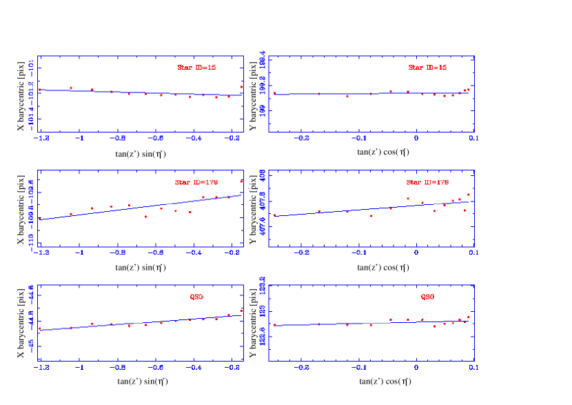
Figure 8: Example DCR series plots for two randomly selected reference stars, and the background QSO J0240-3434B. They are based on a series of 13 off-meridian consecutive frames labeled as “DCR” in Table 1.

As it was done in Costa et al. (2009), a series of “refraction frames” with different values of $(z^{\prime},H^{\prime})$ were acquired for this field (see Table 1). From this series, we then fitted the computed (measured) barycentric positions of all our LRS stars (the left hand side of Equation (6)) as determined from each DCR frame, as a function of $\tan z^{\prime}\sin\eta^{\prime}$, and we computed the straight line fit implied by the right hand side of Equation (6), which allows us to solve for the differential refraction-free coordinates $X_{i,b}$ as the intercept for abscissa zero of that line. An example of this fit, for the QSO and two anonymous stars from the LRS is shown in Figure 8. This figure can be compared to its equivalent, presented by Costa et al. (2009) (their Figure 4), for our PM study of the SMC.

3.4 From pixel coordinates to proper motions; The “QSO method”

Once the LRS coordinates have been corrected for DCR in the way described in the previous section, we can determine the PMs of all our LRS stars and the QSO. The first step at this stage is to build up the SFR mentioned in subsection 3.1. The SFR is constructed from the mean DCR-corrected barycentric coordinates using all the initial LRS stars from the three consecutive, good quality, low-$|HA|$, intermediate-epoch frames indicated as “SFR” in Table 1. We then use a bi-dimensional $(X,Y)$ polynomial fitting routine to compute, based on a $\chi^{2}$ minimization algorithm, transformation equations (coefficients) that map the barycentric DCR-corrected coordinates for the LRS stars (excluding the QSO) from all the frames onto this SFR, and apply these coefficients to transform the coordinates for all the LRS stars and the QSO into the SFR, in the way described by Costa et al. (2009) (specially their Section 3.5). Once the coordinates from all frames haven been transformed into a common reference system (provided by the initial set of 260 LRS stars on the SFR), we perform a simple linear $\chi^{2}$ fit of these coordinates vs. epoch based on all good available frames (see Figure 12). We end up at this stage with PMs for all the LRS stars, and the QSO. In Figure 9 we show the vector point diagram based on all 260 initial LRS stars (see below), as well as for the QSO.

In the method outlined, the underlying assumption is that LRS stars share a common PM so that their coordinates can be registered with high confidence (to the extent of our astrometric accuracy) into a common reference system. The reflex motion of the QSO is measured with respect to this homogenous (kinematically speaking) set of objects, in what is called the “QSO method”. In our case, the expectation is that most of the LRS stars are Fornax members, so the reflex motion of the QSO with respect to the bulk motion of the Fornax stars is nothing but the motion of the galaxy itself with respect to the QSO, which is actually “at rest” (in the tangential direction, which is what concerns us). We cannot however exclude the possibility that a few Galactic foreground stars may be mixed in the LRS. Fortunately, since we have determined PMs for all of the LRS stars, any Galactic star will exhibit a motion different from that of the bulk of Fornax stars. We can therefore start eliminating objects with spuriously high PM, indicative of them not belonging to Fornax. As can be seen form Figure 9 there are actually no objects with extremely large PM: There are only two objects with $\mu>3.0$ mas y^-1, and no objects with $\mu>4.0$ mas y^-1. We note that a typical Galactic halo star would have a PM of $3.0$ mas y^-1 at a distance of 11 kpc. A rather conservative PM cut at $2.0$ mas y^-1 would avoid any halo star out to a Heliocentric distance of 16 kpc equivalent, for the Galactic position of Fornax ($l=237^{o}.1,b=-65^{o}.7$) to a distance of $\sim$15 kpc from the Galactic plane. Given the rather large Galactic latitude of our field, the small FOV, and the magnitude and color range of our selected stars, we expect a rather small Galactic contamination. Indeed, using the Galactic star counts model described by Mendez & van Altena (1996), we predict that there is less than 1 Galactic star per square degree in the range $18\leq R\leq 21.8$ and $0.5\leq B-R\leq 2.5$ (see Figure 10) towards the Fornax field. For our precise FOV, we predict in total 11 Galactic stars satisfying our magnitude & color cuts.

Following the above discussion, we identified 14 LRS stars that satisfy $\mu>2.0$ mas y^-1, and were thus eliminated from the initial LRS, and the full registration (and PMs) for the remaining LRS stars and the QSO re-computed. For comparison purposes, the intermediate PM results for QSO J0240-3434B (catalog ) from these different samples of LRS stars (and for the conditions discussed in the next section) are given in Table 2. As it can be seen, the elimination of these relatively large PM objects did not modify our results substantially. Furthermore, another 7 stars were eliminated from the LRS because they exhibited residuals beyond $3\sigma$ of the formal rms of the registration in at least 4 or more astrometric frames, again the impact of their removal (see Table 2) was minimal.

The PM solution described so far used a full 3^rd degree polynomial in $(X,Y)$ for the registration, and include only the 15 frames satisfying that their $|HA|<1.5$ h, as listed in Table 1, in close resemblance to the strategy adopted in Costa et al. (2009). In the next section we analyze in more detail the stability of our PM solution in regards to these (and other) specific choices.

4 Analysis

In Figures 10 and 11 we show the CMD for the 239 stars of the LRS selected as described in the previous paragraph, as well as the QSO. Throughout this entire paper, our PSF photometry has been approximately calibrated by using a photometric zero point defined by the blue magnitude of the QSO ($B_{\mbox{QSO}}=19.94$) as reported by Tinney et al. (1997). Unfortunately these authors did not report any $R$-band photometry, which was instead scaled by adopting a color for the red-clump on Fornax of $B-R\sim 1.3$, as implied by the deep Fornax photometry from Stetson (1997). Our CMD (plotted for an easy comparison in the same color window as Figure 7 by Stetson (1997)) indicates that Galactic contamination seems to be minimal. In any case, and in order to be absolutely safe and to test the sensitivity of our method to these (possible) outliers, we eliminated the two brightest & reddest objects ($B-R\sim 2.3$), the one object below the Fornax RGB/AGB sequence at $R\sim 20.7$ and $B-R\sim 1.8$, the two faintest & bluest objects at $B-R\sim 0.75$, and finally another two suspicious objects on the upper/left envelope of the AGB/RGB. On the other hand, the PM error vs. magnitude plots (Figure 11) show that there are a few outlier points that can also be eliminated from the LRS. In this case, if we cut at $\sigma_{\mu}>0.5$ mas y^-1 (4 stars), and also eliminate (somewhat subjectively) 11 objects that have unusually large PM error (in either coordinate) for their magnitude (left upper & lower panel on Figure 11), we end up with an LRS sample of 217 stars. The PM solution for this sample, indicated in the 4^th row on Table 2 shows a very small variation with respect to our previous solutions. The variation of the (DCR-corrected) barycentric coordinates for QSO J0240-3434B (catalog ) based on this sample of LRS stars in shown in Figure 12. From now on, this solution will become our “reference value” to carry out the comparisons that follow. Another interesting point brought to mind by Figure 11 is that the QSO shows a perfect agreement with the general trend of PM error vs. magnitude, indicating that its positional uncertainty is no different at all from that of stellar images of the same brightness.

Following the procedure outlined in Costa et al. (2009), all previous PM solutions were computed from frames restricted to being close to the meridian, to avoid any possible unaccounted DCR-related effects. Since, to the best of our ability, we have actually corrected our coordinates of this effect, one may consider including frames outside this range. Given the $|HA|$ distribution of frames in Table 1, increasing the $HA$ window to 2 hours only incorporates two more frames to our solution. While by doing this our errors slightly decrease, the actual PM does not change much. Only by increasing the $HA$ window to 3 hours from the meridian we start to see a larger change in the PM, and a corresponding increase in the overall error of the fit (although the error in PM remains almost constant). Indeed, while the overall rms of the fit in RA and DEC are (0.88,1.27) mas for the $|HA|<1.5$ hrs solution (see Figure 12), this increases to (0.92,1.36) mas for the $|HA|<3.0$ hrs solution. For these reasons, we adopt our original solution, based on the 15 frames with $|HA|<1.5$ hrs. DCR effects are often mentioned in the literature as playing an important role in high-precision ground-based relative astrometry. To illustrate this in the case of our data, we have computed a solution with $|HA|<1.5$ hrs but without any DCR correction (i.e, straight raw pixel coordinates). As we can see on Table 2 the PM values do change somewhat (but, completely within the uncertainties), and the PM errors are slightly increased. In a way this is an expected result, since the data from which the PMs are computed is quite close to the meridian, and therefore the net DCR effect on the motions is not that relevant.

Our coordinates were also pre-corrected for continuous refraction as described in Section 3.3. It can be seen from Equation (1) that since this correction affects only the altitude (not the azimuth) of stellar positions, a failure to correct for this effect could introduce a differential change of scale in the $X$ and $Y$ directions (see Equations (1) and (2) in Costa et al. (2009)). The correction is however small, and it increases with HA of the frame. For example, for the most extreme DCR frame at HA=-4 h (see Table 1), the registration into the SFR frame yields a coefficient for the X-term (which would give the differential scale in the x-coordinate) that differs from 1.0 (= equal scale between the two frames) by $\sim 10^{-4}$ if we pre-correct for continuous refraction. If we do not pre-correct for refraction, the difference to 1.0 becomes $6\times 10^{-4}$. In the y-coordinate the equivalent numbers are $\sim 10^{-4}$ and $7\times 10^{-4}$ respectively. Therefore, the continuous refraction pre-correction does help in rendering the scales more equal (for a given coordinate) for all frames, irrespective of their zenith distance. Another point is that the difference in the x- and y- plate scales is $\sim 10^{-4}$ for the refraction correction coordinates, while this number increases to $5\times 10^{-4}$ if no refraction is applied. Therefore continuous refraction also renders plate scales more equal in both coordinates. We finally note that our registration procedure seems to be able to account for this effect even if no pre-correction is applied, for example, the error in the x- and y- coefficients for the example just described is the same for the corrected and non-corrected data ($\sim 1.5\times 10^{-5}$). In general, if the required ambient data is available, pre-correction for continuous refraction is recommended (William van Altena, private communication).

A critical step in the whole process of obtaining the PMs is to adequately mapping the coordinates from different epochs into the SFR. The SFR itself is built from as many as possible (in our case 3, see Table 1) good-seeing contiguous frames: The average of their barycentric coordinates provides, in principle, a more stable reference system than that of any individual frame, subject to the centroiding errors discussed in section 3.2. Therefore, the SFR better represents the true geometry of the FOV, and allows us to properly map out any offset, rotation, change of scale and, in general, higher order optical distortions between frames of different epochs and the SFR itself. Since we are only concerned with relative displacements as a function of time, by placing the QSO (and of course by extension all the LRS stars) always close to a fiducial reference point near the center of the chip as discussed in section 2, we minimize the relative distortion from different sections of the chip. In our standard procedure (Costa et al., 2009), we take a straight average of the SFR frames, without any registration between them: This might seem justified by the fact that they are contiguous good-quality frames. However, if one computes the scatter of the coordinates for the three frames that contribute to our SFR, we have an rms of $(\sigma_{x},\sigma_{y}=(6.1,2.7)\times 10^{-2}$ pix for the straight average, while this values decreases almost a factor of ten if we do register (quadratically) the SFR frames: $(\sigma_{x},\sigma_{y}=(6.8,6.0)\times 10^{-3}$ pix (in both cases the computed rms is for all the stars brighter than $R~{}\sim 20.7$ discussed in section 3.2). This prompted us to test whether our PM results were sensitive to our straight average of the frames that conform the SFR. For this purpose we created another SFR this time with the three frames that make it registered into one of them by means of a cubic polynomial, and computed our PMs again. The results for the QSO PM (and its error) were equivalent. Therefore, to the level of accuracy of our registration (see next paragraphs), the use of either SFR is completely appropriate.

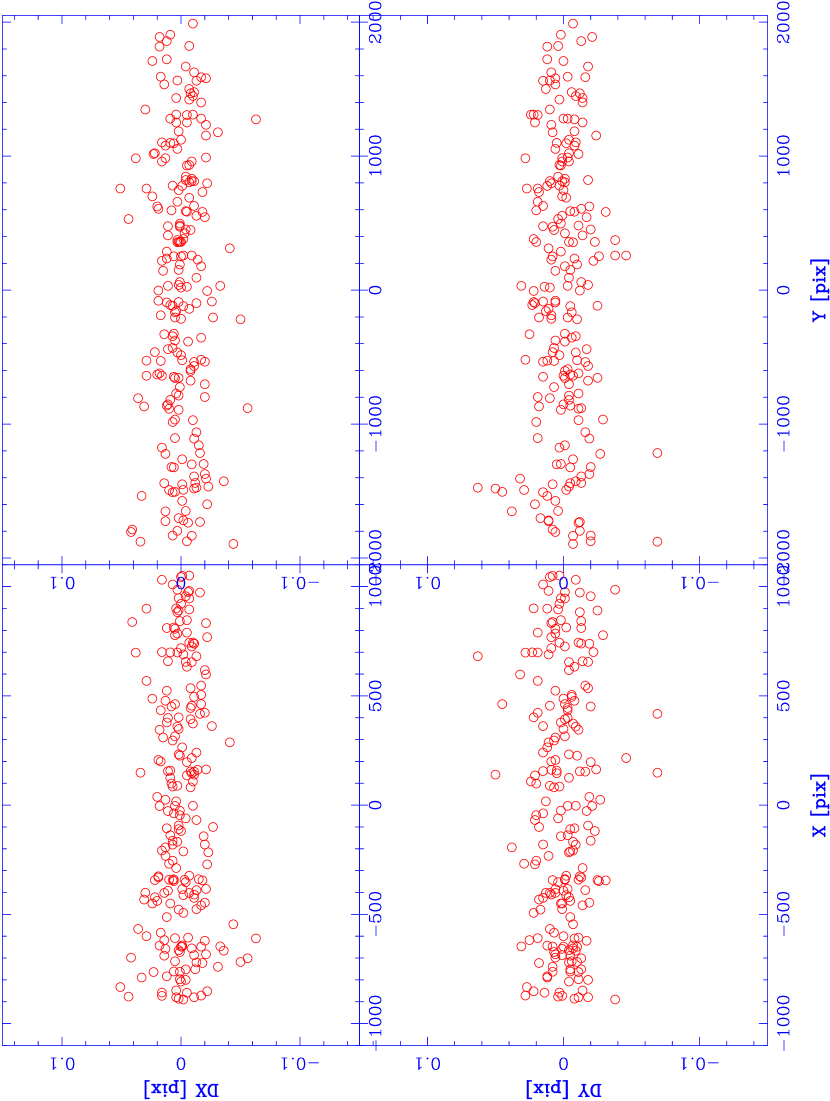
Figure 14: Registration residuals for one of our frames using our 3^rd order registration polynomial. There are no obvious positional trends.

The classical way to discern on the proper modeling of the registration (besides comparing to an external catalog with positions of much higher accuracy than our own - not available in this case) is to look for position-dependent residuals, after registration, as a function of the various relevant positional & flux parameters, and to choose the lowest order correction that, within the uncertainties, leaves no correlations (see, e.g., Figures 9, 10 and 11 in Costa et al. (2009)). In our standard procedure (following Costa et al. (2009)) we have used a full 3^rd order polynomial fit. On the other hand, the PM results, using our “clean” sample of 217 LRS stars when using either a $2^{nd}$ and a $4^{th}$ order polynomial exhibit rather large variations, see Table 2. We can however conclude that, since the PMs are within $1\sigma$ from each other when comparing our 3^rd vs. our $4^{th}$ order polynomial, we would prefer the lower order registration of these two. Deciding between the $2^{nd}$ and 3^rd order registration is less straightforward. We note that in both cases the registration yields rms positional residuals with respect to the LRS of 0.018 pix (as already found in section 3.2), so one might tend, again, to choose the lower $2^{nd}$ order polynomial. We have however reasons to prefer the 3^rd order registration: First, the rms of the barycentric displacement of the QSO has an overall error 5% larger in the $2^{nd}$ order registration ((0.97,1.21) mas in (RA,DEC) respectively) with respect to the 3^rd order registration ((0.88,1.27) mas). Secondly, a plot of the registration coefficients indicates that, at least some of the 3^rd degree coefficients are very significant: In Figure 13 we plot, in logarithmic scale, what we could call the “significance” of each coefficient (given by $\log_{10}(\mbox{Coefficient}/\sigma_{\mbox{\small{coefficient}}})$ of a 3^rd order registration polynomial. As we can see, in the X-coordinate, the only non-significant term seems to be the $Y^{3}$ coefficient, while in the Y-direction, one could perhaps discard the $X^{3}$ and the $XY^{2}$. All other terms appear significant. Even though the specific terms just mentioned seem irrelevant, their inclusion does not hurt our solution: The QSO PM solution leaving these 3^rd order terms out of the registration polynomial produces a solution that is indistinguishable from the full 3^rd order registration (see Table 2), which we then adopt as our standard. An example plot of the registration residuals is shown in Figure 14, as mentioned before the rms of this registration is 0.018 pix.

One other aspect that can seriously affect the registration is the number and distribution of LRS stars. Our LRS stars are randomly distributed all over the field (see Figure 15), but one may wonder whether their number is adequate. If one takes the usual rule-of-thumb that for a $\chi^{2}$ polynomial fit of $N$ coefficients one needs at least $3\times N$ data points, then our number of LRS stars (217) should be plenty to fit our required 10 coefficients per coordinate (see Figure 13). To test the sensitivity of our results to the actual number of LRS stars we performed a solution deleting one every-other entry in the LRS list of stars, ending with 109 LRS stars. The PM solution in this case (see Table 2) indicates a very small change of our results (less than $1\sigma$), showing what we could call a “stable” LRS (i.e. our results are independent of which Fornax stars conform the LRS).

In our method, we calculate PMs for both the QSO (with respect to the motion of the LRS stars), as well as for each LRS star (with respect to the mean of their motion). If all LRS objects are genuine Fornax stars, all these latter motions are not “real” in the sense of not representing any true kinematic signature of Fornax stars, rather they are indicative of our internal errors. Indeed, for a velocity dispersion of a few km s^-1 (typical of the dSphs), this is equivalent, at the distance of 138 kpc (Mateo, 1998), to a proper motion of $\sim 8\mu$as y^-1, much below our measurement uncertainties. Therefore, the “dispersion” of points in the cloud of LRS stars in Figure 9 does not represent true proper motions, but what we could perhaps call “displacements” (or pseudo-PMs, or “residual motions” as in Costa et al. (2009)) due to our various positional measurement uncertainties. For this reason we believe that the use of these displacements to enter into an iterative process to pre-correct the coordinates at different epochs by using the derived pseudo-PMs, and in this way improve the quality of the registration, is not a recommended strategy in this particular case, and we have not implemented it.

In Figures 16 and 17 we plot the (pseudo-)PM for our final sample of 217 LRS stars, and the QSO as a function of position and photometry. As it can be seen from these figures, no significant trends are found. We thus believe that our motions are not affected, as far as we can measure them, by any obvious systematic effects that depend on these parameters.

5 Comparison to other studies & Conclusions

There have been only two astrometric determinations of the PM for the Fornax dSph galaxy, namely that by Dinescu et al. (2004), based on a combination of ground-based plates and Hubble-WFPC data, and that based exclusively on HST data (Piatek et al. (2007), which gives revised values to those reported earlier in Piatek et al. (2002)).

Dinescu et al. (2004), based on an independent determination using 48 galaxies and 8 QSOs give a weighted mean of ($\mu_{\alpha}\cos\delta$,$\mu_{\delta}$)=($0.59\pm 0.16,-0.15\pm 0.16$) mas y^-1. On the other hand, Piatek et al. (2007), based on 4 QSOs (their Table 3), gives a weighted mean of ($\mu_{\alpha}\cos\delta$,$\mu_{\delta}$)=($0.476\pm 0.046,-0.360\pm 0.041$) mas y^-1. In order to compare our result (based on a single QSO) with their measurements it makes more sense to compare our value with their individual PM values. This allows us to estimate the expected uncertainty on our final weighted mean when we incorporate our other 4 QSO fields. In Figure 18 we plot the individual measurements from these previous works, along with our measurement. We note however that, while Piatek et al. (2007) report individual measurements, Dinescu et al. (2004) only give the mean values with respect to 8 QSOs and 48 galaxies, and these are the results plotted in Figure 18. Dinescu et al. (2004) do give the individual PMs for images A and B of the same QSO reported in this paper. These individual values are also plotted in Figure 18. By looking at the open and filled squares we can see the improvement achieved by ground-based astrometry when using CCDs and a homogeneous data set in comparison with the results that combine non-linear plates and heterogeneous data. Nevertheless, it is somewhat surprising how close our (single) value is to the mean PM from galaxies as derived by Dinescu et al. (2004) (differences smaller than $1\sigma$ of our smaller error), while there is a larger discrepancy (although still smaller than $2\sigma$ of their (larger) error) when compared to the PM using QSOs. In Dinescu’s study they have a large sample of brighter better-measured galaxies (see their Figure 2) while the (much fewer) QSOs are fainter and possibly have larger positional errors (although, their individual PM errors are smaller than those of galaxies for a given magnitude all the way down to V$\sim 21$, possibly due to the extended, more diffuse nature of galaxies). Overall, their mean PM with respect to galaxies has an error $\sim 50$% smaller than that derived from the QSOs.

In comparison with the individual HST measurements, we see a rather large discrepancy, specially in DEC: While our value lies between 2.3 and 1.2$\sigma$ away from HST individual PMs in $\mu_{\alpha}\cos\delta$, this difference becomes between 4.4 and 2.4$\sigma$ in $\mu_{\delta}$. We note that the largest & smallest PM values from HST for both $\mu_{\alpha}\cos\delta$ and $\mu_{\delta}$ (see Table 3 on Piatek et al. (2007)) come precisely from images A and B of QSO J0240-3434B (catalog ). Dinescu et al. (2004) also point the rather large discrepancy in the PMs derived from components A and B (plotted in our Figure 18). As was described in section 3.2 the A component of QJ 0240-3434 is indeed affected by two close companions (see Figure 7). It is not unlikely that tiny changes in the photocenter of the images due to other close, unresolved and fainter, companions, or even slightly extended structure(s) in the wings of the QSO (from the underlying QSO galactic disk) could introduce an extra source of noise in the PMs that is not necessarily accounted for in the final PM error budget. Obviously, whether or not our own measurements are subject to some (as yet unknown) systematic effect related to what we just mentioned, is an issue that could be addressed once we incorporate the other QSO fields. In Table 3 we summarize the measurements plotted in Figure 18 (the “perspective” motions are explained further below).

It is interesting to ascertain to what type of final (Heliocentric) velocity errors correspond our individual PM measurement errors. For a given distance and distance error $r\pm\sigma_{r}$ and PM and its error in component “x” (in this case either RA or DEC), $\mu_{x}\pm\sigma_{\mu_{x}}$, the corresponding velocity and its error is given by:

$$v_{x}=K\,r\,\mu_{x}$$ (7)

$$\frac{\sigma_{v_{x}}}{v_{x}}=\sqrt{\left(\frac{\sigma_{r}}{r}\right)^{2}+\left(\frac{\sigma_{\mu_{x}}}{\mu_{x}}\right)^{2}}$$ (8)

where, if $r$ is in kpc, and $\mu_{x}$ is in mas y^-1, then $K=4.74$ and $v_{x}$ and $\sigma_{v_{x}}$ are in km s^-1. According to Mateo (1998), the distance to Fornax is $138\pm 8$ kpc (i.e., 6% formal error). Therefore in equation (8) the distance error is negligible in comparison with our PM errors in either RA or DEC. For our PM reference value (see Table 3) we obtain a Heliocentric velocity and error of $v_{\alpha}=419\pm 58$ km s^-1 and $v_{\delta}=-7\pm 72$ km s^-1. The measured Heliocentric radial velocity from (Mateo, 1998) is $v_{r}=53\pm 3$ km s^-1. It is thus clear that the derived Heliocentric Fornax motion is dominated by uncertainties in the PM from our one-QSO measurement, not by the distance or radial velocity uncertainty. Given our measurement errors, once we incorporate our other four QSO fields, we expect to achieve velocity errors for the weighted mean on the order of 30 km s^-1 per component, totally compatible with the (weighted mean) HST results. Table 3 also shows that our proper motion value exhibits the largest tangential velocity for Fornax after the Dinescu et. al value from Galaxies. At this stage we howevere refrain from making a full analysis of the implications of this result, until we have collected the data from the other four QSO fields which will allow us to have a more robust weighted mean.

We must note that, when comparing PMs values derived for an extended object, such as Fornax, one must actually compare “center-of-mass” (COM) motions to avoid any projection effects and internal galaxy motions (e.g., galactic rotation) that might alter the observed motions. For computing galactic orbits of these galaxies we also need COM velocities. Our measurements are performed, however, on fields away from the COM, and we have to apply corrections to account for this situation. As explained in Costa et al. (2009), in the case of the LMC our PMs had to be corrected not only for projection effects (see below), but also by the effect on our measured PMs induced by the (differential) rotation of the plane of the LMC. To apply these corrections, we followed the prescriptions described by Jones et al. (1994) and van der Marel et al. (2002), which assumed that our fields lay in the plane of the LMC (or SMC) and shared the motion of its disk. The situation for the dSphs is quite different however, they do not exhibit any hint of large-scale rotation, nor of the existence of a disk or other well-defined structure; rather they show a smooth spheroidal distribution and the motion of its stars is dominated by their velocity dispersion, which is typically a few km s^-1 (van den Bergh, 1999). This velocity dispersion translates into a PM dispersion of a few $\mu$as y^-1 which is not measurable by current astrometric techniques (although it will be measured in the future by SIM). Therefore, if we assume that there are no large-scale streaming motions in Fornax, our PMs are not affected, as far as we can measure it, by internal kinematic effects. We do, however, need to correct for purely geometrical projection effects, this is done as described in the following paragraph.

If $(v_{r},v_{\alpha},v_{\delta})$ are the observed (measured) Heliocentric radial velocity, velocity in RA and velocity in DEC respectively, for a field at position $(\alpha,\delta)$ and Heliocentric distance $r$, the velocity for the COM $(v^{*}_{r},v^{*}_{\alpha},v^{*}_{\delta})$ at position $(\alpha^{*},\delta^{*})$ and distance $r^{*}$ is given by:

$$\left(\begin{array}[]{c}v^{*}_{r}\\ v^{*}_{\alpha}\\ v^{*}_{\delta}\end{array}\right)=M^{-1}(\alpha^{*},\delta^{*})\cdot M(\alpha,\delta)\cdot\left(\begin{array}[]{c}v_{r}\\ v_{\alpha}\\ v_{\delta}\end{array}\right)$$ (9)

where $M(\alpha,\delta)$ is a rotation matrix whose components are:

$$M(\alpha,\delta)=\left(\begin{array}[]{ccc}\cos\delta\cos\alpha&-\sin\alpha&-\sin\delta\cos\alpha\\ \cos\delta\sin\alpha&\cos\alpha&-\sin\delta\sin\alpha\\ \sin\delta&0&\cos\delta\end{array}\right)$$ (10)

and which satisfies that $M^{-1}(\alpha,\delta)=M^{t}(\alpha,\delta)$. While $r$ and $r^{*}$ are not explicitely written in equation (9), they are implicitly used to go from PMs to tangential velocities (or vice versa) through equation (7). Of course, $r^{*}=138\pm 8$ kpc. In the case of the LMC (and SMC) Costa et al. (2009) assumed that our fields were located in a disk-like structure with known orientation in the sky (inclination and line of nodes). We do not have however such structures in the featureless dSphs. If we assume, e.g., as a first crude approximation that the galaxy lies in a plane in the sky perpendicular to the line-of-sight to the COM. In this case one can show that $r$ is given by:

$$r=\frac{r^{*}}{\cos\delta\cos\alpha\cos\delta^{*}\cos\alpha^{*}+\cos\delta\sin\alpha\cos\delta^{*}\sin\alpha^{*}+\sin\delta\sin\delta^{*}}$$ (11)

We note that, in equation (9) $v_{r}$ is not known, but we do know $v^{*}_{r}=53\pm 3$ km s^-1 from the literature. Therefore, starting from our measured $v_{\alpha}$ and $v_{\delta}$ values we iterate on the $v_{r}$ values until we reproduce the expected $v^{*}_{r}$ for the COM, in a procedure similar to that adopted by Costa et al. (2009). Also, equations (9) and (10) easily allow us to fully propagate errors on all the measured quantities (radial velocities, proper motions, distances) from the observed values to the sought-for COM values. For our measured PM, the COM distance and radial velocity indicated previously, and the Fornax COM position given by Mateo (1998), we obtain $v^{*}_{\alpha}=419\pm 52$ km s^-1 and $v^{*}_{\delta}=-7\pm 72$ km s^-1, i.e., a value similar to that computed without any projection correction. This is due to the fact that, in this particular case, these corrections are actually quite small, the PM corrections are 0.05 $\mu$as in RA and by 0.45 $\mu$as in DEC. These corrections are, of course, much smaller than the measurement uncertainties involved (this was not case of the LMC and SMC fields reported in Costa et al. (2009)). Note that the field reported here is quite close to the Fornax COM, for some of the other more distant QSO fields in our program, these corrections might be slightly larger, but can be readily computed in each case. None of the values reported by other authors in Table 3 have been corrected for any projection effect, but since these corrections are tiny, one can readily compare them without further corrections.

For completeness, in Table 3 (and in Figure 18), we have included the recent determination of the Fornax PM by Walker et al. (2008), using what they call the “perspective rotation” method (in a way, this method is the reverse of the “astrometric radial velocities”, described by, e.g., Lindegren et al. (2000)). As it can be easily seen from Equations 9 and 10, one could write an equivalent equation for $(v_{r},v_{\alpha},v_{\delta})$ as a function of $(v^{*}_{r},v^{*}_{\alpha},v^{*}_{\delta})$ by a simple matrix inversion. The first row of that equation would give the observed radial velocity $v_{r}$ as a function of a combination of $(v^{*}_{r},v^{*}_{\alpha},v^{*}_{\delta})$ (which, for a given galaxy is of course a fixed quantity - independent of the field observed). Therefore, if one measures the $v_{r}$ of samples of stars at different locations $(\alpha,\delta)$ across a galaxy, one can solve through some minimization algorithm for the unknown $(v^{*}_{r},v^{*}_{\alpha},v^{*}_{\delta})$. Walker et al. (2008) have used precisely this approach to determine the “perspective” PMs for 4 dSphs, including Fornax, using radial velocities exclusively. As it can be seen from Table 3, the method has errors compatible with the best purely astrometric determinations, and can thus become a useful complement to them.

Table 1: Observational material used for the Fornax field centered on QSO J0240-3434B.

Obs. date	Filter	Exp. time	Hour Angle	FWHM	Usage
yyyy-mm-dd		s	hh:mm	arcsec
2000-08-08	B#811	600	-3:40	0.9	CMD
2000-08-08	R#813	360	-1:31	0.6	Astrom
2000-08-08	R#813	360	-1:22	0.5	Astrom
2000-08-08	R#813	250	-0:18	0.5	Astrom, CTB-1
2000-08-08	R#813	250	-0:13	0.5	Astrom, CTB-2
2000-08-08	R#813	250	-0:05	0.5	Astrom
2000-08-08	R#813	300	0:05	0.4	Astrom
2000-08-08	R#813	400	0:15	0.4	Astrom
2004-10-05	R#813	900	0:45	0.6	Astrom, SFR, Master
2004-10-05	R#813	900	1:01	0.6	Astrom, SFR
2004-10-05	R#813	900	1:17	0.6	Astrom, SFR
2005-01-13	R#813	900	1:11	0.8	Astrom
2005-01-13	R#813	900	1:27	0.7	Astrom
2007-11-07	R#813	900	-4:01	0.7	DCR
2007-11-07	R#813	900	-3:40	0.7	DCR
2007-11-07	R#813	900	-3:23	0.7	DCR
2007-11-07	R#813	900	-3:07	0.7	DCR
2007-11-07	R#813	900	-2:51	0.6	DCR
2007-11-07	R#813	900	-2:34	0.6	DCR
2007-11-07	R#813	900	-2:18	0.6	DCR
2007-11-07	R#813	900	-2:01	0.8	DCR
2007-11-07	R#813	900	-1:45	0.8	DCR, Astrom
2007-11-07	R#813	900	-1:28	0.8	DCR, Astrom
2007-11-07	R#813	900	-1:12	0.8	DCR, Astrom
2007-11-07	R#813	900	-0:55	0.7	DCR, Astrom
2007-11-07	R#813	900	-0:38	0.6	DCR, Astrom

Table 2: Proper motion for QSO J0240-3434B under different circumstances explained in detail in the text.

$\mu_{\alpha}\cos\delta$	$\mu_{\delta}$	Comments
mas y-1	mas y-1
$-0.64\pm 0.08$	$0.05\pm 0.11$	All 260 (initial) LRS stars
$-0.66\pm 0.08$	$0.04\pm 0.11$	14 LRS stars with $\mu>2.0$ mas y-1 eliminated (246 LRS stars)
$-0.67\pm 0.08$	$0.01\pm 0.11$	7 stars with high registration residuals eliminated (239 LRS stars)
$-0.64\pm 0.08$	$0.01\pm 0.11$	22 stars eliminated based on CMD & high PM errors (217 LRS stars)
$-0.63\pm 0.07$	$0.05\pm 0.10$	$|HA|\leq 2.0$ hr (17 frames)
$-0.71\pm 0.06$	$0.08\pm 0.09$	$|HA|\leq 3.0$ hr (21 frames)
$-0.71\pm 0.17$	$-0.01\pm 0.11$	$|HA|\leq 1.5$ hr, no DCR correction
$-0.84\pm 0.08$	$0.13\pm 0.10$	2nd order registration
$-0.57\pm 0.07$	$-0.10\pm 0.11$	4th order registration
$-0.63\pm 0.08$	$0.03\pm 0.11$	3rd order registration, no $Y^{3}$ term in X, no $X^{3}$,$XY^{2}$ terms in Y
$-0.58\pm 0.08$	$-0.10\pm 0.14$	Delete one every-other LRS star (109 LRS stars)

Table 3: Proper motion for Fornax from different authors.

$\mu_{\alpha}\cos\delta$	$\mu_{\delta}$	Reference
mas y-1	mas y-1
$0.64\pm 0.08$	$-0.01\pm 0.11$	This work (SuSI2) - J0240-3434B
$0.28\pm 0.30$	$-0.45\pm 0.28$	Dinescu (plates+HST) - mean of 8 QSOs
$0.70\pm 0.18$	$-0.01\pm 0.19$	Dinescu (plates+HST) - mean of 48 Galaxies
$0.541\pm 0.085$	$-0.275\pm 0.071$	Piatek (HST) - J0240-3434A
$0.424\pm 0.096$	$-0.477\pm 0.109$	Piatek (HST) - J0240-3434B
$0.536\pm 0.158$	$-0.325\pm 0.162$	Piatek (HST) - J0240-3438
$0.446\pm 0.072$	$-0.391\pm 0.060$	Piatek (HST) - J0238-3443
$0.48\pm 0.15$	$-0.25\pm 0.14$	Walker - “perspective” motions

Figure 1: Coordinate shifts for the same frame as measured by using two extremely different PSF functional forms. No positional residual trends can be seen.

Figure 2: Same as Figure 1 but as a function of instrumental r-band magnitude and b-r color. A clear trend in the X-coordinate is found as a function of magnitude, and a trend as a function of color is suggested.

Figure 3: Rms of coordinates (dashed lines = X-coordinate, dotted lines = Y-coordinate), derived from the same frame, as a function of the PSF fitting radius. The basic comparison (with $rms=0$, hence the sharp minima seen in the figure) is set at a FWHM of 6.5 pix, equivalent to the seeing of the analyzed frame, CTB-1 in Table 1 (0.5 arcsec). The upper curves are for the entire sample on Figure 2 (i.e., $R\leq 23.2$), whereas the lower curve is for the “well-measured” sample with $R<21$, equivalent to our LRS stars).

Figure 4: Rms of coordinates (dashed lines = X-coordinate, dotted lines = Y-coordinate), derived from two consecutive low-$|HA|$, good-seeing frames (CTB-1 and CTB-2 in Table 1), as a function of the PSF fitting radius. The upper curves are for a sample similar to our LRS system (i.e., $R\leq 23.2$), using a simple linear registration between the two frames, while the lower curve uses a full-quadratic registration and a slightly brighter sample. Both sets of curves show that a value slightly larger than the FWHM should be preferred for the PSF fitting radius. The value adopted throughout this work ($1.2\times$FWHM = 7.5 pix = 0.6 arc-sec in this case) is indicated.

Figure 5: Rms of coordinates in the X-coordinate (upper panel) and Y-coordinate (lower panel), derived from two consecutive small-$|HA|$, good-seeing frames (CTB-1 and CTB-2 in Table 1), as a function of the PSF R-band magnitude for (quadratic) transformation equations obtained using different magnitude cuts (and with correspondingly different rms residuals for the transformation). Dashed line is using all stars down to the same magnitude as the PSF magnitude to compute the transformation equations, solid line is for stars with $R<20.7$ (transformation residuals of 0.027 pix per coordinate, 180 stars used) similar to the LRS stars), dotted is for $R<22.2$ (transformation residuals of 0.061 pix per coordinate, 730 stars used), and dot-dashed for $R<19.7$ (transformation residuals of 0.020 pix per coordinate, 67 stars used).

Figure 6: Various rms noise sources vs. PSF r-band magnitude as measured on CTB-1 within an aperture of 6.5 pixels. Open star, open circle, and open square symbols represent source, sky, and detector (Poisson) noise respectively. Detector noise is negligible in all cases. The small dots indicate the total noise and the asteriscs represent the overall $S/N$ (on an aperture radius of $2timesFWHM$) for each detected object. The “cross-over” when the source noise becomes comparable to the sky noise which indicates when our centering accuracy starts deteriorating rapidly, happens for a $S/N\sim 200$.

Figure 10: CMD for our clean sample (free of high PM stars and registration outliers) comprising 239 LRS stars (dots with PSF photometric error bars), and QSO J0240-3434B (circled dot). This figure, when compared, e.g., with the Fornax deep photometry in Figure 7 by Stetson (1997) indicates that Galactic contamination is minimal. This figure allows us to eliminate LRS objects that due to their magnitude-color combination are unlikely members of Fornax. Moreover, if we compare this figure with, e.g., the Fornax deep photometry in Figure 7 by Stetson (1997) we can see that Galactic contamination is minimal for this field, in agreement with our estimates based on the starcount Galactic model by Mendez & van Altena (1996) (see text).

Figure 11: PM errors for the same sample of LRS as in Figure 10 as a function of magnitude and color. The circled-dot is the QSO. This figure allows us to eliminate LRS objects with unusually large PM errors for their magnitude.

Figure 13: “Significance” (see text for its definition) of each of the polynomial terms (indicated on the abscissa) for our 3^rd order registration. Each point represents one of the 15 frames registered into the SFR. On the right side of the distribution of points we give, for each coefficient, the mean of the significance and its 1$\sigma$ error interval (the error bar). The dotted line represents a significance, in this logarithmic scale, of $\sim 0.477$, equivalent to a coefficient that is 3$\times$ larger than its (formal) error from the $\chi^{2}$ fit. When the average significance (and its interval) are below the dotted line, this indicates non-significant coefficient.

Figure 15: X-Y distribution of our final 217 LRS stars (open star symbol). The $+$ symbol indicates 43 initial LRS stars that were subsequently purged for various reasons, discussed in the text. Both sets of stars are distributed over the entire FOV.

Figure 16: Proper motions vs. X- and Y-coordinates for the final 217 LRS stars (dots) and the QSO (circle). No obvious trends vs. position in the frames are discernible.

Figure 17: Same as Figure 16 but vs. magnitude and color. Other than the expected increase in (pseudo-) PMs for the LRS stars (see text) at fainter magnitudes, and the much bluer color of the QSO with respect to the Fornax stars, no obvious trends are found.

Figure 18: Comparison of Fornax PMs. The open stars are the HST values from Piatek et al. (2007) from 4 individual QSOs, the filled and open circle are the mean PMs using 8 QSOs and 48 galaxies respectively from the Plates+HST/WFPC study from Dinescu et al. (2004), and the filled square is our single measurement on QSO J0240-3434B. The open squares are the individual measurements reported in the Dinescu et al. (2004) paper for both components (image A and B) of the same QSO reported by us in this study. We also include (filled star) the recent result by Walker et al. (2008) (see Table 3) obtained through the “perspective” proper motion method using radial velocities alone, and further discussed in the text (note that, in a way, this should be considered a measurement based on a weighted mean of many lines of sight - using in total 2,610 Fornax stars). As it can be seen our value is closer to the Dinescu et al. (2004) determination using galaxies rather than their value using QSOs. Also, our single measurement errors are similar to those from HST.

References

- Anderson et al. (2006) Anderson, J., Bedin, L. R., Piotto, G., Yadav, R. S., & Bellini, A. 2006, A&A, 454, 1029
- Besla et al. (2007) Besla, G., Kallivayalil, N., Hernquist, L., Robertson, B., Cox, T.J, van der Marel, R.P., Alcock, C. 2007, ApJ668, 949
- Bristow et al. (2006) Bristow, P., Kerber, F., & Rosa, M. R. 2006, The 2005 HST Calibration Workshop: Hubble After the Transition to Two-Gyro Mode, 299 (available at http://www.stsci.edu/hst/HST_overview/documents/calworkshop/workshop2005/papers/cws05proc.pdf)
- Byrd et al. (1994) Byrd, G., Valtonen, M., McCall, M. & Innanen, K. 1994, AJ, 107, 2055
- Carlin et al. (2009) Carlin, J. L., Grillmair, C. J., Muñoz, R. R., Nidever, D. L., Majewski, S. R. 2009, ApJ, 702, L9
- Costa et al. (2009) Costa, E., Méndez, R. A., Pedreros, M. H., Moyano, M., Gallart, C., Noël, N., Baume, G., & Carraro, G. 2009, AJ, 137, 4339
- Dinescu et al. (2000) Dinescu, D. I., Majewski, S. R., Girard, T. M., Cudworth, K. M. 2000, AJ, 120, 1892
- Dinescu et al. (2004) Dinescu, D. I., Keeney, B. A., Majewski, S. R., & Girard, T. M. 2004, AJ, 128, 687
- D’Odorico (1998) D’Odorico, S., 1998, The ESO Messenger, 91, 14
- D’Odorico et al. (1998) D’Odorico, S., Beletic, J. W., Amico, P., Hook, I., Marconi, G., & Pedichini, F. 1998, Proc. SPIE, 3355, 507
- Hodge (1961) Hodge, P. W. 1961, AJ, 66, 83
- Jones et al. (1994) Jones, B. F., Klemola, A. R., & Lin, D. N. C. 1994, AJ, 107, 1333
- Lindegren et al. (2000) Lindegren, L., Madsen, S., & Dravins, D. 2000, A&A, 356, 1119
- Lynden-Bell (1982) Lynden-Bell, D. 1982, Obs. 102, 202
- Lynden-Bell and Lynden-Bell (1995) Lynden-Bell, D. & Lynden-Bell, R.M. 1995, MNRAS, 275, 429
- Massey and Davies (1992) Massey, P. and Davis, L. 1992. “A User’s Guide to Stellar CCD Photometry with IRAF”
- Mateo (1998) Mateo, M. 1998, ARA&A, 36, 435
- Mayer (2010) Mayer, L. 2010, Advances in Astronomy, 2010, 1
- Mendez & van Altena (1996) Mendez, R. A., & van Altena, W. F. 1996, AJ, 112, 655
- Noël et al. (2009) Noël, N. E. D., Aparicio, A., Gallart, C., Hidalgo, S. L., Costa, E., Méndez, R. A. 2009, ApJ, 705, 1260
- Palma et al. (2002) Palma, C., Majewski, S.R., Johnston, K.V. 2002, ApJ, 564, 736
- Piatek et al. (2002) Piatek, S., et al. 2002, AJ, 124, 3198
- Piatek et al. (2005) Piatek, S., Pryor, C., Bristow, P., Olszewski, E. W., Harris, H. C., Mateo, M., Minniti, D., Tinney, C. G. 2005, AJ, 130, 95
- Piatek et al. (2007) Piatek, S., Pryor, C., Bristow, P., Olszewski, E. W., Harris, H. C., Mateo, M., Minniti, D., & Tinney, C. G. 2007, AJ, 133, 818
- Peebles (1989) Peebles, P.J.E. 1989, ApJ, 344, 53
- Peebles (1994) Peebles, P.J.E. 1994, ApJ, 429, 43
- Smarts (1962) Smarts, W.M. 1962, TextBook on Spherical Astronomy, Cambridge at the University Press, fifth edition
- Stetson (1997) Stetson, P. B. 1997, Baltic Astronomy, 6, 3
- Stone (1996) Stone, R. C. 1996, PASP, 108, 1051
- Taff (1991) Taff, L.G. 1991, Computational Spherical Astronomy, Krieger Publishing Company, Reprinted with corrections
- Tinney et al. (1997) Tinney, C. G., Da Costa, G. S., & Zinnecker, H. 1997, MNRAS, 285, 111
- Tinney (1995) Tinney, C. G. 1995, MNRAS, 277, 609
- Unwin et al. (2008) Unwin, S.C. et al. 2008, PASP, 120, 38
- van den Bergh (1999) van den Bergh, S. 1999, The Stellar Content of Local Group Galaxies, 192, 3
- van der Marel et al. (2002) van der Marel, R. P., Alves, D. R., Hardy, E., & Suntzeff, N. B. 2002, AJ, 124, 2639
- van Leeuwen et al. (2000) van Leeuwen, F., Le Poole, R. S., Reijns, R. A., Freeman, K. C., & de Zeeuw, P. T. 2000, A&A, 360, 472
- Walker et al. (2008) Walker, M. G., Mateo, M., & Olszewski, E. W. 2008, ApJ, 688, L75
- Zaritsky and Harris (2004) Zaritsky, D. & Harris, J. 2004, ApJ, 604, 167