Analog Matching of Colored Sources to Colored Channels

Abstract

Analog (uncoded) transmission provides a simple and robust scheme for communicating a Gaussian source over a Gaussian channel under the mean squared error (MSE) distortion measure. Unfortunately, its performance is usually inferior to the all-digital, separation-based source-channel coding solution, which requires exact knowledge of the channel at the encoder. The loss comes from the fact that except for very special cases, e.g. white source and channel of matching bandwidth (BW), it is impossible to achieve perfect matching of source to channel and channel to source by linear means. We show that by combining prediction and modulo-lattice operations, it is possible to match any colored Gaussian source to any colored Gaussian noise channel (of possibly different BW), hence achieve Shannon’s optimum attainable performance $R(D)=C$. Furthermore, when the source and channel BWs are equal (but otherwise their spectra are arbitrary), this scheme is asymptotically robust in the sense that for high signal-to-noise ratio a single encoder (independent of the noise variance) achieves the optimum performance. The derivation is based upon a recent modulo-lattice modulation scheme for transmitting a Wyner-Ziv source over a dirty-paper channel.

keywords: joint source/channel coding, analog transmission, Wyner-Ziv problem, writing on dirty paper, modulo lattice modulation, MMSE estimation, prediction, unknown SNR, broadcast channel, ISI channel, bandwidth expansion/reduction.

I Introduction

Digital transmission of analog sources relies, at least from a theoretical point of view, on Shannon’s source-channel separation principle. Being both optimal and easy to implement, digital techniques replace today traditional analog communication even in areas like voice telephony, radio and television. This trend ignores, however, the fact that the separation principle does not hold for communication networks, and in particular for broadcast channels and compound channels [6, 37, 29]. Indeed, due to both practical and theoretical reasons, joint source-channel coding and hybrid digital-analog schemes are constantly receiving attention of researchers in the academia and the industry.

In this work we consider transmission under the mean-squared error (MSE) distortion criterion, of a general stationary Gaussian source over a power-constrained channel with inter-symbol interference (ISI), i.e. the transmitted signal is passed through some linear filter, and additive white Gaussian noise (AWGN).

Shannon’s joint source-channel coding theorem implies that the optimal (i.e., minimum distortion) performance $D^{opt}$ is given by

$$R\left(D^{opt}\right)=C,$$ (1)

where $R(D)$ is the rate-distortion function of the source at MSE distortion $D$, and $C=C(P)$ is the channel capacity at power-constraint $P$, both given by the well-known water-filling solutions [6]. By Shannon’s separation principle, (1) can be achieved by a system consisting of source and channel coding schemes. This system usually requires large delay and complex digital codes. An additional serious drawback of the all-digital system is that it suffers from a “threshold effect”: if the channel noise turns out to be higher than expected, then the reconstruction will suffer from very large distortion, while if the channel has lower noise than expected, then there is no improvement in the distortion [37, 29, 2].

In contrast, analog communication techniques (like amplitude or frequency modulation [5]) are not sensitive to exact channel knowledge at the transmitter. Moreover, in spite of their low complexity and delay, they are sometimes optimal: if we are allowed one channel use per source sample, and the source and noise are white (i.e. have i.i.d. samples), then a “single-letter” coding scheme achieves the optimum performance of (1), see e.g. [11]. In this scheme, the transmitter consists of multiplication by a constant factor that adjusts the source to the power constraint $P$, so it is independent of the channel parameters. Only the receiver needs to know the power of the noise in order to optimally estimate the source from the noisy channel output (by multiplying by the “Wiener coefficient”).

For the case of colored sources and channels, however, such a simple solution is not available, as single-letter codes are only optimal in very special scenarios [10]. A particular case is when the channel bandwidth is not equal to the source bandwidth, but otherwise they are white (i.e., a white source is sent through an AWGN channel with some average number of channel uses per source sample). As it turns out, even if we consider more general linear transmission schemes, [1], still (1) is not achievable in the general colored case. How far do we need to deviate from “analog” transmission in order to achieve optimal performance in the colored case? More importantly, can we still achieve full robustness?

In this work we propose and investigate a semi-analog transmission scheme. This scheme achieves the optimum performance of (1) for any colored source and channel pair without explicit digital coding, hence we call it the Analog Matching (AM) scheme. Furthermore, for the matching bandwidth case ($B_{C}=B_{S}$, but arbitrary source and channel spectra), we show that the Analog Matching transmitter is asymptotically robust in the high signal-to-noise ratio (SNR) regime, in the sense that it becomes invariant to the variance of the channel noise. Thus, in this regime, the perfect SNR-invariant matching property of white sources and channels [11] generalizes to the equal-BW colored case.

Previous work on joint source/channel coding for the BW-mismatch/colored setting mostly consists of hybrid digital analog (HDA) solutions, which involve splitting the source or channel into frequency bands, or using a superposition of encoders (see [25, 18, 24, 22, 19] and references therein), mostly for the cases of bandwidth expansion ($B_{C}>B_{S}$) and bandwidth compression ($B_{C}<B_{S}$) with white spectra. Most of these solutions, explicitly or implicitly, allocate different power and bandwidth resources to analog and digital source representations, thus they still employ full digital coding. Other works [2, 30] treat bandwidth expansion by mapping each source sample to a sequence of channel inputs independently; by the scalar nature of these mappings, they do not aim at optimal performance.

In contrast to HDA solutions, the AM scheme treats the source and channel in the time domain, using linear prediction, thus it also has the potential of shorter delay. Furthermore, it does not involve any quantization of the source or digital channel code, but rather it applies modulo-lattice arithmetic to analog signals. This modulation allows to take advantage of side information - here based on prediction - while keeping the analog nature of transmission.

Problem	Conventional prediction	Side-information based solution
Source coding	DPCM compression	WZ video coding
Channel coding	FFE-DFE receiver	Dirty-paper coding = precoding
Joint source-channel coding	Does not exist	Analog matching

TABLE I: *

Table I: Information-Theoretic time-domain solutions to colored Gaussian source and channel problems.

Table I demonstrates the place of the Analog Matching scheme within information-theoretic time-domain schemes. For the separate colored Gaussian source and channel problems, digital coding schemes, based upon the combination of prediction and memoryless codebooks, are optimal: differential pulse code modulation (DPCM) in source coding (see [13] for basic properties and [35] for optimality), and feed-forward-equalizer / decision-feedback-equalizer (FFE-DFE) receiver in channel coding (see [3]).

The optimality of DPCM hinges on prediction being performed using the reconstruction rather than the source itself. Identical predictors, with equal outputs, are employed at the encoder and at the decoder. An alternative approach, advocated for low-complexity encoding, is “Wyner-Ziv video coding” (see e.g. [23]). In this approach, prediction is performed at the decoder only and is treated as decoder side-information [32]. In the context of the AM scheme, however, decoder-only prediction is not an option but a must: since no quantization is used, but rather the reconstruction error is generated by the channel, the encoder does not have access to the error and the side-information approach must be taken.

In the channel counterpart, the FFE-DFE receiver cancels the effect of past channel inputs by filtering past decoder decisions (assumed to be equal to these inputs). In order to avoid error propagation, sometimes precoding [27], where the filter is moved to the encoder, is preferred; this can be seen as a form of dirty-paper coding [4] , where the filter output plays the role of encoder side-information. Again, the AM scheme must use the “encoder side-information” variant: if no channel code is used, then the decoder cannot make digital decisions regarding past channel inputs, so virtually it has no access to these inputs.

Figure 1: *

Figure 1: Workings of the AM scheme in the high-SNR limit. The source is assumed to have an auto-regressive (AR) model. $\mod\Lambda$ is the modulo-lattice operation.

To summarize, the AM scheme uses source prediction at the decoder, and channel prediction at the encoder, and then treats the predictor outputs as Wyner-Ziv and dirty-paper side-information, respectively; see Figure 1. Digital solutions to these side-information problems rely on binning, which may also be materialized in a structured (lattice) way [36]. AM treats these two side-information problems jointly using modulo-lattice modulation (MLM) , an approach proposed recently for joint Wyner-Ziv and dirty-paper coding [15]. However, combining these pieces turns out to be a non-trivial task. The interaction of filters with high-dimensional lattice codes raises technical difficulties which are solved in the sequel.

The rest of the paper is organized as follows: We start in Section II by bringing preliminaries regarding sources and channels with memory, as well as modulo-lattice modulation and side-information problems. In Section III we prove the optimality of the Analog Matching scheme. In Section IV we analyze the scheme performance for unknown SNR, and prove its asymptotic robustness. Finally, Section V discusses applications of AM, and is advantage relative to other approaches (e.g. HDA) in terms of delay.

II Formulation and Preliminaries

In Section II-A we formally present the problem. In the rest of the section we bring preliminaries necessary for the rest of the paper. In Sections II-B to II-D we present results connecting the Gaussian-quadratic rate-distortion function (RDF) and the Gaussian channel capacity to prediction, mostly following [35]. In sections II-E and II-F we discuss lattices and their application to joint source/channel coding with side information, mostly following [15].

II-A Problem Formulation

Figure 2: *

Figure 2: Colored Gaussian joint source/channel setting.

Figure 2 demonstrates the setting we consider in this paper. The source $S_{n}$ is zero-mean stationary Gaussian, with spectrum $S_{S}({e^{j2\pi f}})$. As for the channel, for the purpose of the analysis to follow we break away with the ISI model discussed in the introduction, and use a colored noise model:

$$Y_{n}=X_{n}+Z_{n},$$ (2)

where $X_{n}$ and $Y_{n}$ are the channel input and output, $Z_{n}$ is zero-mean additive stationary Gaussian noise with spectrum $S_{Z}({e^{j2\pi f}})$, assumed to be finite for all $2|f|\leq B_{C}$ and infinite otherwise. The channel input $X_{n}$ needs to satisfy the power constraint $\mathop{\mathrm{Var}}\{X_{n}\}\leq P$, and the distortion of the reconstruction $\hat{S}_{n}$ is given by $D=\mathop{\mathrm{Var}}\{\hat{S}_{n}-S_{n}\}$.

II-B Spectral Decomposition and Prediction

Let $A_{n}$ be a zero-mean discrete-time stationary process, with power spectrum $S_{A}({e^{j2\pi f}})$. The Paley-Wiener condition is given by [28]:

$$\left|\int_{-\frac{1}{2}}^{\frac{1}{2}}\log\Bigl{(}S_{A}({e^{j2\pi f}})\Bigr{)}df\right|<\infty\ \ ,$$ (3)

where here and in the sequel logarithms are taken to the natural base. It holds for example if the spectrum $S_{A}({e^{j2\pi f}})$ is bounded away from zero. Whenever the Paley-Wiener condition holds, the spectrum has a spectral decomposition:

$$S_{A}({e^{j2\pi f}})=\left.Q(z)Q^{*}\left(\frac{1}{z^{*}}\right)\right|_{z=j2\pi f}P_{e}\Bigl{(}S_{A}\Bigr{)}\ \ ,$$ (4)

where $Q(z)$ is a monic causal filter, and the entropy-power $P_{e}\left(S_{A}\right)$ of the spectrum is defined by:

$$P_{e}(S_{A})\stackrel{{\scriptstyle\Delta}}{{=}}P_{e}\Bigl{(}S_{A}({e^{j2\pi f}})\Bigr{)}=\exp{\int_{-\frac{1}{2}}^{\frac{1}{2}}\log\Bigl{(}S_{A}({e^{j2\pi f}})\Bigr{)}df}\ \ .$$ (5)

The optimal predictor of the process $A_{n}$ from its infinite past is

$$P(z)=1-Q^{-1}(z)\ \ ,$$ (6)

a filter with an impulse response satisfying $p_{n}=0$ for all $n\leq 0$. The prediction mean squared error (MSE) is equal to the entropy power of the process:

$$\mathop{\mathrm{Var}}\{A_{n}|A_{-\infty}^{n-1}\}=P_{e}(S_{A})\ \ .$$ (7)

The prediction error process can serve as a white innovations process for AR representation of the process.

We define the prediction gain of a spectrum $S_{A}({e^{j2\pi f}})$ as:

$$\Gamma(S_{A})\stackrel{{\scriptstyle\Delta}}{{=}}\Gamma\Bigl{(}S_{A}({e^{j2\pi f}})\Bigr{)}\stackrel{{\scriptstyle\Delta}}{{=}}\frac{\int_{-\frac{1}{2}}^{\frac{1}{2}}S_{A}({e^{j2\pi f}})df}{P_{e}\left(S_{A}\right)}=\frac{\mathop{\mathrm{Var}}\{A_{n}\}}{\mathop{\mathrm{Var}}\{A_{n}|A_{-\infty}^{n-1}\}}\geq 1\ \ ,$$ (8)

where the gain equals one if and only if the spectrum is white, i.e. fixed over all frequencies $|f|\leq\frac{1}{2}$. A case of special interest, is where the process is band-limited such that $S_{A}({e^{j2\pi f}})=0\ \forall|f|>\frac{B}{2}$ where $B<1$. In that case, the Paley-Wiener condition (3) does not hold and the prediction gain is infinite. We re-define, then, the prediction gain of a process band-limited to $B$ as the gain of the process downsampled by $\frac{1}{B}$, i.e.,

$$\Gamma(S)=\frac{\frac{1}{B}\int_{-\frac{B}{2}}^{\frac{B}{2}}S_{A}({e^{j2\pi f}})df}{\exp\left[\frac{1}{B}\int_{-\frac{B}{2}}^{\frac{B}{2}}\log\Bigl{(}S_{A}({e^{j2\pi f}})\Bigr{)}df\right]}\ \ .$$ (9)

We will use in the sequel prediction from a noisy version of a process: Suppose that $C_{n}=A_{n}+W_{n}$, with $W_{n}$ additive white with power $\theta$. Then it can be shown that the noisy prediction error has variance (see e.g. [35]):

$$\mathop{\mathrm{Var}}\{A_{n}|C_{-\infty}^{n-1}\}=P_{e}(S_{A}+\theta)-\theta\ \ .$$ (10)

Note that for any $\theta>0$, the spectrum $S_{A}({e^{j2\pi f}})+\theta$ obeys (3), so that the conditional variance is non-zero even if $A_{n}$ is band-limited. In the case $\theta=0$, (10) collapses to (7).

II-C Water-Filling Solutions and the Shannon Bounds

The RDF for a Gaussian source with spectrum $S_{S}({e^{j2\pi f}})$ under an MSE distortion measure is given by:

$$R(D)=\frac{1}{2}\int_{-\frac{1}{2}}^{\frac{1}{2}}\log\frac{S_{S}({e^{j2\pi f}})}{D({e^{j2\pi f}})}df\ \ ,$$ (11)

where the distortion spectrum $D({e^{j2\pi f}})$ is given by the reverse water-filling solution: $D({e^{j2\pi f}})=\min\Bigl{(}\theta_{S},S({e^{j2\pi f}})\Bigr{)}$ with the water level $\theta_{S}$ set by the distortion level $D$:

$$D=\int_{-1/2}^{1/2}D({e^{j2\pi f}})df\ \ \ .$$

The Shannon lower bound (SLB) for the RDF of a source band-limited to $B_{S}$ is given by:

$$R(D)\geq\frac{B_{S}}{2}\log\frac{{\text{SDR}}}{\Gamma_{S}}\stackrel{{\scriptstyle\Delta}}{{=}}R_{SLB}(D)\ \ ,$$ (12)

where SDR, the signal-to-distortion ratio, is defined as:

$${\text{SDR}}\stackrel{{\scriptstyle\Delta}}{{=}}\frac{\mathop{\mathrm{Var}}\{S_{n}\}}{D}$$ (13)

and $\Gamma_{S}\stackrel{{\scriptstyle\Delta}}{{=}}\Gamma(S_{S})$ is the source prediction gain (9). This bound is tight for a Gaussian source whenever the distortion level $D$ is low enough such that $D<B_{S}\min_{|f|\leq B_{S}}S_{S}({e^{j2\pi f}})$, and consequently $D({e^{j2\pi f}})=\theta_{S}=\frac{D}{B_{S}}$ for all $|f|<B_{S}$. Note that the bound reflects a coding rate gain of $B_{S}/2\log(\Gamma_{S})$ with respect to the RDF of a white Gaussian source.

The capacity of the colored channel (2) where the noise $Z_{n}$ has spectrum $S_{Z}({e^{j2\pi f}})$, bandlimited to $B_{C}$, is given by:

$$C=\int_{-\frac{B_{C}}{2}}^{\frac{B_{C}}{2}}{\log\left(1+\frac{P({e^{j2\pi f}})}{S_{Z}({e^{j2\pi f}})}\right)}\ \ ,$$ (14)

where the optimum channel input spectrum $P({e^{j2\pi f}})$ is given by the water-filling solution: $P({e^{j2\pi f}})=\max\Bigl{(}\theta_{C}-S_{Z}({e^{j2\pi f}}),0\Bigr{)}$ inside the band, with the water level $\theta_{C}$ set by the power constraint $P$:

$$P=\int_{-B_{C}/2}^{B_{C}/2}P({e^{j2\pi f}})df\ \ \ .$$

The Shannon upper bound (SUB) for the channel capacity is given by:

$$C\leq\frac{B_{C}}{2}\log\left[\Gamma_{C}\cdot\left(1+{\text{SNR}}\right)\right]\stackrel{{\scriptstyle\Delta}}{{=}}C_{SUB}\ \ ,$$ (15)

where SNR, the signal-to-noise ratio, is defined as:

$${\text{SNR}}\stackrel{{\scriptstyle\Delta}}{{=}}\frac{P}{N}\stackrel{{\scriptstyle\Delta}}{{=}}\frac{P}{\int_{-B_{C}/2}^{B_{C}/2}{S_{Z}({e^{j2\pi f}})}df}\ \ ,$$ (16)

and $\Gamma_{C}\stackrel{{\scriptstyle\Delta}}{{=}}\Gamma(S_{Z})$ is the channel prediction gain (8). The bound is tight for a Gaussian channel whenever the SNR is high enough such that $P\geq B_{C}\max_{|f|\leq B_{C}}S_{Z}({e^{j2\pi f}})-N$ and consequently $S_{Z}({e^{j2\pi f}})+P({e^{j2\pi f}})=\theta_{C}=\frac{P+N}{B_{C}}$. Note that the bound reflects a coding rate gain of $B_{C}/2\log(\Gamma_{C})$ with respect to the AWGN channel capacity.

We now connect the capacity and RDF expressions. In terms of the SDR and SNR defined above, and denoting the inverse of the RDF by $R^{-1}(\cdot)$, the optimal performance (1) becomes:

$${\text{SDR}}^{opt}\stackrel{{\scriptstyle\Delta}}{{=}}\frac{\mathop{\mathrm{Var}}\{S_{n}\}}{R^{-1}(C({\text{SNR}}))}\ \ .$$ (17)

Let the bandwidth ratio be

$$\rho\stackrel{{\scriptstyle\Delta}}{{=}}\frac{B_{C}}{B_{S}}\ \ .$$ (18)

Combining (12) with (15), we have the following asymptotically tight upper bound on the Shannon optimum performance. It shows that the prediction gains product $\Gamma_{S}\Gamma_{C}$ gives the total SDR gain relative to the case where the source and channel spectra are white.

Proposition 1

$$\frac{SDR^{opt}}{(1+{\text{SNR}})^{\rho}}\leq\Gamma_{S}\Gamma_{C}\ \ ,$$

with equality if and only if the SLB and SUB both hold with equality. Furthermore, if the source and the channel noise both satisfy the Paley-Wiener condition (3) inside their respective bandwidths, then when the SNR is taken to infinity by increasing the power constraint $P$ while holding the noise spectrum fixed:

$$\lim_{{\text{SNR}}\rightarrow\infty}\frac{{\text{SDR}}^{opt}}{{\text{SNR}}^{\rho}}=\Gamma_{S}\Gamma_{C}\ \ .$$ (19)

II-D Predictive Presentation of the Gaussian RDF and Capacity

(a) RDF-achieving configuration using filters and AWGN channel.

(b) Capacity-achieving configuration using filters and white Gaussian input.

Figure 3: *

Figure 3: Forward-channel configurations for the RDF and capacity.

Not only the SLB and SUB in (12) and (15) can be written in predictive forms, but also the rate-distortion function and channel capacity, in the Gaussian case. These predictive forms are given in terms of the forward-channel configurations depicted in Figure 3b.

For source coding, let $F_{1}({e^{j2\pi f}})$ be any filter with amplitude response satisfying

$$|F_{1}({e^{j2\pi f}})|^{2}=1-\frac{D({e^{j2\pi f}})}{S_{S}({e^{j2\pi f}})}\ \ ,$$ (20)

where $D({e^{j2\pi f}})$ is the distortion spectrum materializing the water-filling solution (11). We call $F_{1}({e^{j2\pi f}})$ and $F_{2}({e^{j2\pi f}})=F_{1}^{*}({e^{j2\pi f}})$ the pre- and post-filters for the source $S$ [34].

As a consequence of (10), the pre/post filtered AWGN depicted in Figure 3a satisfies [35]:

$$R(D)=\frac{1}{2}\log\left(1+\frac{\mathop{\mathrm{Var}}\{U_{n}|V_{-\infty}^{n-1}\}}{\mathop{\mathrm{Var}}\{Z_{n}\}}\right)\ \ ,$$ (21)

where ${\mathop{\mathrm{Var}}\{Z_{n}\}}=\theta_{S}$. Note that in the limit of low distortion the filters vanish, prediction from $U_{n}$ is equivalent to prediction from $V_{n}$, and we go back to (12). Defining the source Wiener coefficient

$$\alpha_{S}=1-\exp\left(-2R(D)\right)\ \ ,$$ (22)

(21) implies that

$$\mathop{\mathrm{Var}}\{U_{n}|V_{-\infty}^{n-1}\}=\frac{\alpha_{S}}{1-\alpha_{S}}\theta_{S}\ \ .$$ (23)

For channel coding, let $G_{1}({e^{j2\pi f}})$ be any filter with amplitude response satisfying

$$|G_{1}({e^{j2\pi f}})|^{2}=\frac{P({e^{j2\pi f}})}{\theta_{C}}\ \ ,$$ (24)

where $P({e^{j2\pi f}})$ and $\theta_{C}$ are the channel input spectrum and water level materializing the water-filling solution (14). $G_{1}({e^{j2\pi f}})$ is usually referred to as the channel shaping filter, but motivated by the the similarity with the solution to the source problem we call it a channel pre-filter. At the channel output we place $G_{2}({e^{j2\pi f}})=G_{1}^{*}({e^{j2\pi f}})$, known as a matched filter, which we call a channel post-filter.

In the pre/post filtered colored-noise channel depicted in Figure 3b, let the input $\tilde{X}_{n}$ be white and define the (non-Gauusian, non-additive) noise $\tilde{Z}_{n}=\tilde{Y}_{n}-\tilde{X}_{n}$. Then the channel satisfies (see [9], [35]):

$$C=\frac{1}{2}\log\left(\frac{\mathop{\mathrm{Var}}\{\tilde{X}_{n}\}}{\mathop{\mathrm{Var}}\{\tilde{Z}_{n}|{\tilde{Z}}_{-\infty}^{n-1}\}}\right)$$ (25)

where $\mathop{\mathrm{Var}}\{\tilde{X}_{n}\}=\theta_{C}$. Note that in the limit of low noise the filters vanish, prediction from $\tilde{Z}_{n}$ is equivalent to prediction from $Z_{n}$, and we go back to (15). Defining the channel Wiener coefficient

$$\alpha_{C}=1-\exp\left(-2C\right)\ \ ,$$ (26)

(25) implies that

$$\mathop{\mathrm{Var}}\{\tilde{Z}_{n}|{\tilde{Z}}_{-\infty}^{n-1}\}=\frac{1-\alpha_{C}}{\alpha_{C}}\theta_{C}\ \ .$$ (27)

Combining (22) with (26), we note that in a joint source-channel setting where the optimum performance (1) is achieved,

$$\alpha_{S}=\alpha_{C}=\alpha\ \ .$$ (28)

A connection between the water-filling parameters and conditional variances can be derived using (23) and (27).

The predictive presentations (21) and (25) translate the process mutual information rates $\bar{I}(S_{n};\hat{S}_{n})$ and $\bar{I}(X_{n};Y_{n})$ to the conditional mutual informations $I(U_{n};V_{n}|V_{-\infty}^{n-1})$ and $I(\tilde{X}_{n};\tilde{X}_{n}+\tilde{Z}_{n}|\tilde{Z}_{-\infty}^{n-1})$, respectively. This is highly attractive as the basis for coding schemes, since it allows to use the combination of predictors and generic optimal codebooks for white sources and channels, regardless of the actual spectra, without compromising optimality. See e.g. [12], [35]. In the source case, (21) establishes the optimality of a DPCM-like scheme, where the prediction error of $U_{n}$ from the past samples of $V_{n}$ is being quantized and the quantizer is equivalent to an AWGN. For channel coding, (25) implies a noise-prediction receiver, which can be shown to be equivalent to the better known MMSE FFE-DFE solution [3].

II-E Good Lattices for Quantization and Channel Coding

Let $\Lambda$ be a $K$-dimensional lattice, defined by the generator matrix $G\in\mathbb{R}^{K\times K}$. The lattice includes all points $\{{\bf l}=G\cdot{\bf i}:{\bf i}\in\mathbb{Z}^{K}\}$ where $\mathbb{Z}=\{0,\pm 1,\pm 2,\ldots\}$. The nearest neighbor quantizer associated with $\Lambda$ is defined by

$$Q({\bf x})=\arg\min_{{\bf l}\in\Lambda}\|{\bf x}-{\bf l}\|\ \ ,$$

where ties are broken in a systematic way. Let the basic Voronoi cell of $\Lambda$ be

$${\mathcal{V}}_{0}=\{{\bf x}:Q({\bf x})=\textbf{0}\}\ \ .$$

The second moment of a lattice is given by the variance of a uniform distribution over the basic Voronoi cell, per dimension:

$$\sigma^{2}(\Lambda)=\frac{1}{K}\cdot\frac{\int_{{\mathcal{V}}_{0}}\|{\bf x}\|^{2}d{\bf x}}{\int_{{\mathcal{V}}_{0}}d{\bf x}}\ \ .$$ (29)

The modulo-lattice operation is defined by:

$${\bf x}\bmod{\Lambda}={\bf x}-Q({\bf x})\ \ .$$

The following is the key condition that has to be verified in the analysis to follow.

Definition 1

(Correct decoding) We say that correct decoding of a vector ${\bf x}$ by a lattice $\Lambda$ occurs, whenever

$${\bf x}\bmod\Lambda={\bf x}\ \ ,$$

i.e., ${\bf x}\in{\mathcal{V}}_{0}$.

For a dither vector ${\bf d}$ which is independent of ${\bf x}$ and uniformly distributed over the basic Voronoi cell ${\mathcal{V}}_{0}$, $[{\bf x}+{\bf d}]\bmod{\Lambda}$ is uniformly distributed over ${\mathcal{V}}_{0}$ as well, and is independent of ${\bf x}$ [33].

We assume the use of lattices which are simultaneously good for source coding (MSE quantization) and for AWGN channel coding [7]. Roughly speaking, a sequence of $K$-dimensional lattices is good for MSE quantization if the second moment of these lattices tends to that of a uniform distribution over a ball of the same volume, as $K$ grows. A sequence of lattices is good for AWGN channel coding if the probability of correct decoding (1) of a Gaussian i.i.d. vector with element variance smaller than the square radius of a ball having the same volume as the lattice basic cell, approaches zero for large $K$. There exists a sequence of lattices satisfying both properties simultaneously, thus for these lattices, correct decoding holds with high probability for Gaussian i.i.d. vectors with element variance smaller than $\sigma^{2}(\Lambda)$, for large enough $K$. This property also holds when the Gaussian vector is replaced by a linear combination of Gaussian and “self noise” (uniformly distributed over the lattice basic cell) components. The following formally states the property used in the sequel.

Definition 2

(Combination noise) Let ${\bf Z}_{1},\ldots,{\bf Z}_{L}$ be mutually-i.i.d. vectors, independent of ${\bf Z}_{0}$, uniformly distributed over the basic cell of $\Lambda$, and let ${\bf Z}_{0}$ be a Gaussian i.i.d. vector with element variance $\sigma^{2}(\Lambda)$. Then for any real coefficients, $\sum_{l=0}^{L}\alpha_{l}{\bf z}_{L}$ is a combination noise with composition $\alpha_{0},\ldots,\alpha_{L}$.

Proposition 2

(Existence of good lattices) Let $\{\Lambda_{K}\}$ denote a sequence of $K$-dimensional lattices with basic cells $\{{\mathcal{V}}_{K}\}$ of fixed second moment $\sigma^{2}$. Let $\{{\bf Z}_{K}\}$ be a corresponding sequence of combination noise vectors, with fixed composition satisfying:

$$\sum_{l=1}^{L}\alpha_{l}^{2}<1\ \ .$$

Then there exists a sequence $\{\Lambda_{K}\}$ such that:

$$\limsup_{K\rightarrow\infty}\Pr\{{\bf Z}_{K}\bmod\Lambda_{K}\neq{\bf Z}_{k}\}=0\ \ .$$

This is similar to [15, Poposition 1], but with the single “self-noise” component replaced by a combination. It therefore requires a proof, included in the appendix.

II-F Coding for the Joint WZ/DPC Problem using Modulo-Lattice Modulation

Figure 4: *

Figure 4: The Wyner-Ziv / dirty-paper coding problem.

(a) The MLM scheme.

(b) Asymptotic equivalent real-additive channel for “good” lattices. The equivalent noise ${\bf Z}_{eq}=\alpha{\bf Z}-(1-\alpha){\bf X}$ is independent of ${\bf Q}$, and asymptotically Gaussian.

Figure 5: *

Figure 5: MLM Wyner-Ziv / dirty-paper coding.

The lattices discussed above can be used for achieving the optimum performance in the joint source/channel Gaussian Wyner-Ziv/dirty-paper coding, depicted in Figure 4. In that problem, the source is the sum of an unknown i.i.d. Gaussian component $Q_{n}$ and an arbitrary component $J_{n}$ known at the decoder, while the channel noise is the sum of an unknown i.i.d. Gaussian component $Z_{n}$ and an arbitrary component $I_{n}$ known at the encoder. In [15] the MLM scheme of Figure 5a is shown to achieve the optimal performance (1) for suitable $\alpha$ and $\beta$. This is done showing asymptotic equivalence with high probability (for good lattices) to the real-additive channel of Figure 5b. The output-power constraint $P$ in that last channel reflects the element variance condition in order to ensure correct decoding of the vector $\beta{\bf Q}_{n}+{{\bf Z}_{eq}}_{n}$ with high probability, according to Proposition 2. When this holds, the dithered modulo-lattice operation at the encoder and the decoder perfectly cancel each other. This way, the MLM scheme asymptotically translates the SI problem to the simple problem of transmitting the unknown source component $Q_{n}$ over an AWGN, where the known source component $J_{n}$ and the channel interference $I_{n}$ are not present.

III The AM Scheme

Figure 6: *

Figure 6: The Analog Matching scheme.

In this section we prove the optimality of the Analog Matching scheme, depicted in Figure 6, in the limit of high lattice dimension. We assume for now that we have $K$ mutually-independent identically-distributed source-channel pairs in parallel, which allows a $K$-dimensional dithered modulo-lattice operation across these pairs. Other operations are done independently in parallel. To simplify notation we omit the index $k$ of the source/channel pair ($k=1,2,\ldots,K$), and use scalar notation meaning any of the $K$ pairs; we denote by bold letters $K$-dimensional vectors, for the modulo-lattice operation. Subscripts denote time instants. Under this notation, the AM encoder is given by:

$${{U}_{n}} = {f_{1}}_{n}*{{S}_{n}}$$

$$\tilde{\bf X}_{n} = \left[\beta{\bf U}_{n}-{\bf I}_{n}+{\bf D}_{n}\right]\bmod\Lambda$$

$${{I}_{n}} = -\sum_{m=1}^{\infty}{p_{C}}_{m}\tilde{X}_{n-m}$$

$${{X}_{n}} = {g_{1}}_{n}*{{\tilde{X}}_{n}}\ \ ,$$ (30)

while the decoder is given by:

$${{\tilde{Y}}_{n}} = {g_{2}}_{n}*{{Y}_{n}}$$

$${{Y^{\prime}}_{n}} = {{\tilde{Y}}_{n}}-\sum_{m=1}^{\infty}{p_{C}}_{m}\tilde{Y}_{n-m}$$

$${\bf V}_{n} = \frac{1}{\beta}\left[\tilde{\bf Y}_{n}-\beta{\bf J}_{n}-{\bf D}_{n}\right]\bmod\Lambda+{\bf J}_{n}$$

$${{J}_{n}} = \sum_{m=1}^{\infty}{p_{S}}_{k}V_{n-k}$$

$${{\hat{S}}_{n}} = {f_{2}}_{n}*{{V}_{n}}\ \ ,$$ (31)

where $*$ denotes convolution. For each filter of frequency response $H({e^{j2\pi f}})$, the corresponding impulse response is denoted by small letters $h_{n}$. Each of the $K$ parallel channels is given by the colored noise model (2).

The filters used in the scheme are determined by the optimal solutions presented in Sections II-C and II-D. The channel capacity, and corresponding water-level $\theta_{C}$, are given by (14). This determines, through the optimality condition (1), the distortion level $D$. Using that $D$, the RDF, and corresponding water-level $\theta_{S}$, are given by (11). The filters $F_{1}({e^{j2\pi f}})$ and $F_{2}({e^{j2\pi f}})$ are then chosen according to (20), and $G_{1}({e^{j2\pi f}})$ and $G_{2}({e^{j2\pi f}})$ according to (24). We also use $\alpha$ of (28). Finally, $P_{S}({e^{j2\pi f}})$ and $P_{C}({e^{j2\pi f}})$ are the optimal predictors (6) of the spectra

$$S_{V}({e^{j2\pi f}})\stackrel{{\scriptstyle\Delta}}{{=}}|F_{1}({e^{j2\pi f}})|^{2}S_{S}({e^{j2\pi f}})+\frac{1-\alpha}{\beta^{2}}\theta_{C}$$ (32)

and

$$S_{\tilde{Z}}({e^{j2\pi f}})\stackrel{{\scriptstyle\Delta}}{{=}}\ \Bigl{(}1-|G_{1}({e^{j2\pi f}})|^{2}\Bigr{)}^{2}\theta_{C}+|G_{1}({e^{j2\pi f}})|^{2}S_{Z}({e^{j2\pi f}})\ \,$$ (33)

respectively, where we take $|G_{1}({e^{j2\pi f}})|^{2}S_{Z}({e^{j2\pi f}})=0$ wherever $|G_{1}({e^{j2\pi f}})|=0$ even if $S_{Z}({e^{j2\pi f}})$ is infinite.

The analysis we apply to the scheme shows that at each time instant it is equivalent to a joint source/channel side-information (SI) scheme, and then applies the Modulo-Lattice Modulation (MLM) approach presented in Section II-F. The key to the proof is showing that with high probability the correct decoding event of Definition 1 holds, thus the modulo-lattice operation at the decoder exactly cancels the corresponding operation at the encoder. As the distribution of the signal fed to the decoder modulo-lattice operation depends upon the past decisions through the filters memory, the analysis has a recursive nature: we show, that if the scheme is in a “correct state” at time instant $n$, it will stay in that state at instant $n+1$ with high probability, resulting in optimal distortion. Formally, for the decoder modulo-lattice input:

$${\bf T}_{n}=\beta({\bf U}_{n}-{\bf J}_{n})+{{\bf Z}_{eq}}_{n}\ \ ,$$ (34)

we define the desired state as follows.

Definition 3

We say that the Analog Matching scheme is correctly initialized at time instance $n$, if all signals at all times $n-1,n-2,\ldots$ take values according to the assumption that correct decoding (see Definition 1) held w.r.t. ${\bf T}_{n-1},{\bf T}_{n-2},\ldots$.

Using this, we make the following optimality claim.

Theorem 1

(Asymptotic optimality of the Analog Matching scheme) Let $D(N,K)$ be the achievable expected distortion of the AM scheme operating on input blocks of time duration $N$ with lattice dimension $K$. Then there exists a sequence $N(K)$ such that

$$\lim_{K\rightarrow\infty}D(N(K),K)=D^{opt}\ \ ,$$

where $D^{opt}$ was defined in (1), provided that at the start of transmission the scheme is correctly initialized.

In Section III-A we gain some insight into the workings of the scheme by considering it in the uqual-BW high-SNR regime, while in Section III-B we cosider the important special cases of bandwidth expansion and compression. Section III-C contains the proof of Theorem 1, and then in Section III-D we discuss how one can implement a scheme based on the theorem.

III-A The Scheme in the Equal-BW High-SNR Regime

In the equal-BW case ($B_{S}=B_{C}$) and in the limit of high resolution ($D^{opt}\ll P_{e}(S_{S})$), the scheme can be simplified significantly. In this limit, the filters approach zero-forcing ones: both source and channel pre- and post-filters collapse to unit all-pass filters, while the source and channel predictors become just the optimal predictors of the spectra $S_{S}({e^{j2\pi f}})$ and $S_{Z}({e^{j2\pi f}})$, respectively. The receiver filter $1-P_{C}(z)$ is then a whitening filter for the noise, and the channel from $X_{n}$ to $Y^{\prime}_{n}$ is equivalent to a white-noise inter-symbol interference (ISI) channel:

$$Y^{\prime}_{n}=X_{n}-\sum_{m=1}^{\infty}{p_{C}}_{m}X_{n-m}+W_{n}\ \ ,$$ (35)

where $W_{n}$ is AWGN of variance $P_{e}(S_{Z})$. Under these conditions, the source can always be modeled as an auto-regressive (AR) process:

$$S_{n}=\sum_{m=1}^{\infty}{p_{S}}_{m}S_{n-m}+Q_{n}\ \ ,$$ (36)

where $Q_{n}$ is the white innovations process, of power $P_{e}(S_{S})$.

Figure 7: *

Figure 7: The scheme in the high-SNR limit.

The resulting scheme is depicted in Figure 7. It is evident, that the channel predictor cancels all of the ISI, while the source predictor removes the source memory, so that effectively the scheme transmits the source innovation through an AWGN channel. The gains of source and channel prediction are $\Gamma_{S}=P_{e}(S_{S})/\mathop{\mathrm{Var}}\{S_{n}\}$ and $\Gamma_{C}=P_{e}(S_{Z})/\mathop{\mathrm{Var}}\{Z_{n}\}$, respectively (recall (8)). In light of (19), the product of the two is indeed the required gain over memoryless transmission. In fact, if we assume that the modulo-lattice operations have no effect, then the entire scheme is equivalent to the AWGN channel:

$$\hat{S}_{n}=S_{n}+\frac{W_{n}}{\beta}\ \ .$$

Letting $\beta^{2}=P/\mathop{\mathrm{Var}}\{Q_{n}\}$, we than have that:

$${\text{SDR}}=\frac{\beta^{2}\mathop{\mathrm{Var}}\{S_{n}\}}{\mathop{\mathrm{Var}}\{W_{n}\}}=\frac{\beta^{2}\Gamma_{C}{\text{SNR}}\mathop{\mathrm{Var}}\{S_{n}\}}{P}=\Gamma_{S}\Gamma_{C}{\text{SNR}}$$

which is optimal at the limit, recall (19). In order to satisfy the power constraint, the lattice second moment must be $P$, thus the gain $\beta$ amplifies the source innovations to a power equal to the lattice second moment; as we will prove in the sequel, this choice of $\beta$ indeed guarantees correct decoding, on account of Proposition 2.

III-B The BW Mismatch Case

At this point, we present the special cases of bandwidth expansion and bandwidth compression, and see how the analog matching scheme specializes to these cases. In these cases the source and the channel are both white, but with different bandwidth (BW). The source and channel prediction gains are both one, and the optimum condition (17) becomes:

$${\text{SDR}}^{opt}=\left(1+{\text{SNR}}\right)^{\rho}\ \ ,$$ (37)

where the bandwidth ratio $\rho$ was defined in (18).

For bandwidth expansion ($\rho>1$), we choose to work with a sampling rate corresponding with the channel bandwidth, thus in our discrete-time model the channel is white, but the source is band-limited to a frequency of $\frac{1}{2\rho}$. As a result, the channel predictor $P_{C}(z)$ vanishes and the channel post-filters become the scalar Wiener factor $\alpha$. The source water-filling solution allocates all the distortion to the in-band frequencies, thus we have $\theta_{S}=\rho D$ and the source pre- and post-filters become both ideal low-pass filters of width $\frac{1}{2\rho}$ and height

$$\sqrt{1-\frac{1}{{\text{SDR}}^{opt}}}=\sqrt{1-\frac{1}{\left(1+{\text{SNR}}\right)^{\rho}}}\ \ .$$ (38)

As the source is band-limited, the source predictor is non-trivial and depends on the distortion level. The resulting prediction error of $U_{n}$ has variance

$$\mathop{\mathrm{Var}}\{U_{n}|V_{-\infty}^{n-1}\}=\frac{\rho\mathop{\mathrm{Var}}\{S_{n}\}}{\left(1+{\text{SNR}}\right)^{\rho-1}}\ \ ,$$

and the resulting distortion achieves the optimum (37).

For bandwidth compression ($\rho<1$), the sampling rate reflects the source bandwidth, thus the source is white but the channel is band-limited to a frequency of $B_{C}=\frac{\rho}{2}$. In this case the source predictor becomes redundant, and the pre- and post-filters become a constant factor equal to (38). The channel pre- and post-filters are ideal low-pass filter of width $\frac{\rho}{2}$ and unit height. The channel predictor is the SNR-dependent DFE. Again this results in achieving the optimum distortion (37). It is interesting to note, that in this case the outband part of the channel error ${{\tilde{Z}}_{n}}$ is entirely ISI (a filtered version of the channel inputs), while the inband part is composed of both channel noise and ISI, and tends to be all channel noise at high SNR.

III-C Proof of Theorem 1

We start the optimality proof by showing that the Analog Matching scheme is equivalent at each time instant to a WZ/DPC scheme, as in Section II-F. Specifically, the equivalent scheme is shown in Figure 8a, which bears close resemblance to Figure 5a. The equivalence is immediate using the definitions of $I_{n}$ (III) and $J_{n}$ (III), since they are constructed in the encoder and the decoder using past values of $\tilde{X}_{n}$ and $V_{n}$, respectively, thus at any fixed time instant they can be seen as side information. It remains to show that indeed the unknown noise component is white, and evaluate its variance.

Lemma 1

(Equivalent side-information scheme) Assume that $\mathop{\mathrm{Var}}{\tilde{X}_{n}}=\theta_{C}$, then

$${{Z^{\prime}}_{n}}\stackrel{{\scriptstyle\Delta}}{{=}}\frac{Y^{\prime}_{n}-I_{n}}{\alpha}-\tilde{X}_{n}$$

is a white process, independent of all $U_{n}$, with variance

$$\mathop{\mathrm{Var}}\{Z^{\prime}_{n}\}=\frac{1-\alpha}{\alpha}\theta_{C}\ \ .$$

(a) Equivalent WZ/DPC scheme.

(b) Equivalent modulo-lattice channel.

(c) Asymptotic equivalent scalar additive channel for good lattices.

Figure 8: *

Figure 8: Equivalent channels for the Analog Matching scheme.

The proof of this lemma appears in the appendix. Now we note, that if the modulo-lattice operations in the equivalent scheme of Figure 8a can be dropped, this will result in a scalar additive white-noise channel (see Figure 8c):

$$V_{n}=U_{n}+\frac{{Z_{eq}}_{n}}{\beta}\ \ ,$$ (39)

where

$${Z_{eq}}_{n}=\alpha Z^{\prime}_{n}-(1-\alpha)\tilde{X}_{n}$$ (40)

is a white additive noise term of variance

$$\mathop{\mathrm{Var}}\{{Z_{eq}}_{n}\}=\alpha\mathop{\mathrm{Var}}\{Z^{\prime}_{n}\}=(1-\alpha)\theta_{C}\ \ .$$ (41)

Together with the source pre/post filters $F_{1}({e^{j2\pi f}})$ and $F_{2}({e^{j2\pi f}})$, we can have the forward test channel of Figure 3a. Furthermore, if $\beta^{2}$ equals

$$\beta_{0}^{2}\stackrel{{\scriptstyle\Delta}}{{=}}(1-\alpha)\frac{\theta_{C}}{\theta_{S}}$$ (42)

then the additive noise variance is $\theta_{S}$, resulting in optimal performance. The relevant condition is that correct decoding (recall Definition 1) holds for ${\bf T}_{n}$ (34). Using the concept of correct initialization (Definition 3), we first give a recursive claim.

Lemma 2

(Steady-state behavior of the Analog Matching scheme) Assume that the Analog Matching scheme is applied, using a lattice $\Lambda=\Lambda_{K}$ of dimension $K$ which is taken from a sequence of lattices of second moment $\theta_{C}$ which are simultaneously good for source and channel coding in the sense of Proposition 2. Then the probability that correct decoding does not hold in the present instance can be bounded by $p_{e}(K)$, where

$$\lim_{K\rightarrow\infty}p_{e}(K)=0\ \ ,$$

given that the scheme is correctly initialized and that $\beta>\beta_{0}$ (42).

Now we translate the conditional result above (again proven in the appendix), to the optimality claim for blocks.

Proof of Theorem 1: We choose $N(K)$ to be some sequence such that

$$\lim_{K\rightarrow\infty}N(K)=\infty\ \ ,$$

but at the same time

$$\lim_{K\rightarrow\infty}N(K)p_{e}(K)=0\ \ ,$$

where $p_{e}(K)$ was defined in Lemma 2. Let $D^{correct}$ and $D^{incorrect}$ be the expected distortion given that the scheme remains correctly initialized at the end of transmission or does not, respectively. By the union bound we have that:

$$D(N(K),K)\leq D^{correct}(N(K),K)+N(K)p_{e}(K)D^{incorrect}(N(K),K)\ \ .$$

Since we assumed that $N(K)p_{e}(K)$ vanishes in the limit of infinite $K$, so does the second term; see [15, Appendix II-B]. We thus have that

$$\lim_{K\rightarrow\infty}D(N(K),K)=\lim_{K\rightarrow\infty}D^{correct}(N(K),K)$$

and we can assume that (39) holds throughout the block. This results in the forward channel of Figure 3a, up to two issues. First, the channel is stationary while transmission has finite duration, and second the additive noise variance is larger than $\theta_{S}$ since $\beta>\beta_{0}$. The first may be solved by forcing $U_{n}$ and $V_{n}$ to be zero outside the transmission block, resulting in an excess distortion term; however this finite term vanishes when averaging over large $N(K)$. The second implies that $D^{opt}+\epsilon$ may still be achieved for any $\epsilon>0$, and the result follows by a standard arguments, replacing $\epsilon$ by a sequence $\epsilon(K)\rightarrow 0$

III-D From the Idealized Scheme to Implementation

We now discuss how the scheme can be implemented with finite filters, how the correct initialization assumption may be dropped, and how the scheme may be used for a single source/channel pair.

1. Filter length. If we constrain the filters to have finite length, we may not be able to implement the optimum filters. However, it is possible to show, that the effect on both the correct decoding condition and the final distortion can be made as small as desired, since the additional signal errors due to the filters truncation can be all made to have arbitrarily small variance by taking long enough filters. In the sequel we assume the filters all have length $L$.

2. Initialization. After taking finite-length filters, we note that correct initialization now only involves a finite history of the scheme. Consequently, we can create this state by adding a finite number of channel uses. Now we may create a valid state for the channel predictor $P_{C}({e^{j2\pi f}})$ by transmitting $L$ values $\tilde{X}_{n}=0$; see [12]. For the source predictor the situation is more involved, since in absence of past values of ${{V}_{n}}$, the decoder cannot reduce the source power to the innovations power, and correct decoding may not hold. This can be solved by de-activating the predictor for the first $L$ values of $U_{n}$, and transmitting them with lower $\beta$ such that (54) holds without subtracting $J_{n}$. Now in order to achieve the desired estimation error for these first values of $V_{n}$, one simply repeats the same values of $U_{n}$ a number of times according to the (finite) ratio of $\beta$’s. If the block length $N$ is long enough relative to $L$, the number of excess channel uses becomes insignificant.

3. Single source/channel pair. A pair of interleaver/de-interleaver can serve to emulate $K$ parallel sources, as done in [12] for an FFE-DFE receiver, and extended to lattice operations in [36]. Interestingly, while a separation-based scheme which employs time-domain processing for both source and channel parts requires two separate interleavers, one suffices for the AM scheme. Together with the initialization process, we have the following algorithm.

encoder:

1. Write $U_{n}$ row-wise into an interleaving table.

2. Before each row, add source initialization samples.

3. Build a table for $\tilde{X}_{n}$, starting by zero columns for channel initialization. Then add more columns using column-wise modulo-lattice operations on the table of $U_{n}$, using row-wise past values of $\tilde{X}_{n}$ as inputs to the channel predictor.

4. Feed the $\tilde{X}_{n}$ table to the channel pre-filter row-wise.

decoder:

1. Write $Y^{\prime}_{n}$ row-wise.

2. Discard the first columns, corresponding to channel initialization.

3. Build a table for $V_{n}$, starting by using the source initialization data. Then add more columns using column-wise modulo-lattice operations on the table of $Y^{\prime}_{n}$, using row-wise past values of $V_{n}$ as inputs to the source predictor.

4. Feed the $V_{n}$ table to the source post-filter row-wise.

IV Unknown SNR

So far we have assumed in our analysis that both the encoder and decoder know the source and channel statistics. In many practical communications scenarios, however, the encoder does not know the channel, or equivalently, it needs to send the same message to different users having different channels. Sometimes it is assumed that the channel filter $H_{0}({e^{j2\pi f}})$ is given, but the noise level $N$ is only known to satisfy $N\leq N_{0}$ for some given $N_{0}$. For this special case, and specifically the broadcast bandwidth expansion and compression problems, see [25, 18, 24, 22].

Throughout this section, we demonstrate that the key factor in asymptotic behavior for high SNR is the bandwidth ratio $\rho$ (18). We start in Section IV-A by proving a basic lemma regarding achievable performance when the encoder is not optimal for the actual channel. In the rest of the section we utilize this result: in Section IV-B we show asymptotic optimality for unknown SNR in the case $\rho=1$, then in Section IV-C we show achievable performance for the special cases of (white) BW expansion and compression, and finally in Section IV-D we discuss general spectra in the high-SNR limit.

IV-A Basic Lemma for Unknown SNR

We prove a result which is valid for the transmission of a colored source over a degraded colored Gaussian broadcast channel: We assume that the channel is given by (2), where $B_{C}$ is known but the noise spectrum $S_{Z}({e^{j2\pi f}})$ is unknown, except that it is bounded from above by some spectrum $S_{Z0}({e^{j2\pi f}})$ everywhere. We then use an Analog Matching encoder optimal for $S_{Z0}({e^{j2\pi f}})$, as in Theorem 1, but optimize the decoder for the actual noise spectrum. Correct decoding under $S_{Z0}({e^{j2\pi f}})$ ensures correct decoding under $S_{Z}({e^{j2\pi f}})$, thus the problem reduces to a linear estimation problem, as will be evident in the proof.

For this worst channel $S_{Z0}({e^{j2\pi f}})$ and for optimal distortion (17), we find the water-filling solutions (11),(14), resulting in the source and channel water levels $\theta_{S}$ and $\theta_{C}$ respectively, and in a source-channel passband ${\cal F}_{0}$, which is the intersection of the inband frequencies of the source and channel water-filling solutions:

$${\cal F}_{S} = \{f:S_{S}({e^{j2\pi f}})\geq\theta_{S}\}\ \ ,$$

$${\cal F}_{C} = \{f:S_{Z_{0}}({e^{j2\pi f}})\leq\theta_{C}\}\ \ ,$$

$${\cal F}_{0} = {\cal F}_{S}\cap{\cal F}_{C}\ \ .$$ (43)

Under this notation we have the following lemma, proven in the appendix. It shows that the resulting distortion spectrum is that of a linear scheme which transmits the source into a channel with noise spectrum $P/\Phi({e^{j2\pi f}})$, where

$$\Phi({e^{j2\pi f}})=\frac{S_{Z_{0}}({e^{j2\pi f}})}{S_{Z}({e^{j2\pi f}})}\left[1-\frac{S_{Z_{0}}({e^{j2\pi f}})-S_{Z}({e^{j2\pi f}})}{\theta_{C}}\right]\frac{S_{S}({e^{j2\pi f}})-\theta_{S}}{\theta_{S}}\ \$$

depends on both the design noise spectrum and the actual one.

Lemma 3

For any noise spectrum $S_{Z0}({e^{j2\pi f}})$, there exists an encoder, such that for any equivalent noise spectrum

$$S_{Z}({e^{j2\pi f}})\leq S_{Z0}({e^{j2\pi f}})\ \forall\ f\in{\cal F}_{C}\ \ ,$$ (44)

a suitable decoder can arbitrarily approach:

$$D=\int_{-\frac{1}{2}}^{\frac{1}{2}}D({e^{j2\pi f}})df\ \ ,\vspace{-2mm}$$

where the distortion spectrum $D({e^{j2\pi f}})$ satisfies:

$${D({e^{j2\pi f}})}=\left\{\begin{array}[]{ll}\frac{S_{S}({e^{j2\pi f}})}{1+\Phi({e^{j2\pi f}})},&\mbox{if $f\in{\cal F}_{0}$}\\ \min\Bigl{(}S_{S}({e^{j2\pi f}}),\theta_{S}\Bigr{)},&\mbox{otherwise}\end{array}\right\}\ \ .$$ (45)

Remarks:

1. Outside the source-channel passband ${\cal F}_{0}$, there is no gain when the noise spectrum density is lower than expected. Inside ${\cal F}_{0}$, the distortion spectrum is strictly monotonously decreasing in $S_{Z}({e^{j2\pi f}})$, but the dependence is never stronger than inversely proportional. It follows, that the overall SDR is at most linear with the SNR. This is to be expected, since all the gain comes from linear estimation.

2. In the unmatched case modulation may change performance. That is, swapping source frequency bands before the analog matching encoder will change ${\cal F}_{0}$ and $\Phi({e^{j2\pi f}})$, resulting in different performance as $S_{Z}({e^{j2\pi f}})$ varies. It can be shown that the best robustness is achieved when $S_{S}({e^{j2\pi f}})$ is monotonously decreasing in $S_{Z}({e^{j2\pi f}})$.

3. The degraded channel condition (44) is not necessary. A tighter condition for correct decoding to hold can be stated in terms of $S_{S}({e^{j2\pi f}})$, $S_{Z0}({e^{j2\pi f}})$ and $S_{Z}({e^{j2\pi f}})$: the integral over $S_{eq}({e^{j2\pi f}})$, defined in the appendix (55), must be at most as it is for the spectrum $S_{0}({e^{j2\pi f}})$.

IV-B Asymptotic Optimality for equal BW

We prove asymptotic optimality in the sense that, if in an ISI channel (recall (35)), the ISI filter is known but the SNR is only known to be above some ${\text{SNR}}_{0}$, then a single encoder can simultaneously approach optimality for any such SNR, in the limit of high $SNR_{0}$.

Theorem 2

(High-SNR robustness) Let the source and channel have BW $B_{S}=B_{C}=1$, and let the equivalent ISI model of the channel (35) have fixed filter coefficients (but unknown innovations power $\mathop{\mathrm{Var}}\{W_{n}\}$). Then, there exists an SNR-independent sequence of encoders indexed by their lattice dimension $K$, each achieving ${\text{SDR}}_{K}({\text{SNR}})$, such that for any $\delta>0$:

$$\lim_{K\rightarrow\infty}{\text{SDR}}_{K}({\text{SNR}})\geq(1-\delta){\text{SDR}}^{opt}({\text{SNR}})$$

for sufficiently large (but finite) SNR, i.e., for all ${\text{SNR}}\geq{\text{SNR}}_{0}(\delta)$.

Proof:

The limit of a sequence of encoders is required, since any fixed finite-dimensional encoder has a gap from ${\text{SDR}}^{opt}$ that would limit performance as ${\text{SNR}}\rightarrow\infty$. At the limit, however, we may assume an ideal scheme. In terms of the colored noise channel (2), the unknown noise variance in the theorem conditions is equivalent to having noise spectrum

$$S_{Z}({e^{j2\pi f}})=\frac{{\text{SNR}}_{0}}{{\text{SNR}}}S_{Z0}({e^{j2\pi f}})$$

where ${\text{SNR}}\geq{\text{SNR}}_{0}={\text{SNR}}_{0}(\delta)$. We apply Lemma 3, with an encoder designed for $S_{Z0}({e^{j2\pi f}})$. If the source spectrum is bounded away from zero and the $S_{Z0}({e^{j2\pi f}})$ is bounded from above, we can always take ${\text{SNR}}_{0}$ high enough such that the source-channel passband ${\cal F}_{0}$ includes all frequencies, and then we have for all ${\text{SNR}}\geq{\text{SNR}}_{0}$:

$$D({e^{j2\pi f}})\leq\frac{1}{1-\delta}\cdot\frac{{\text{SNR}}_{0}}{{\text{SNR}}}\theta_{S}$$

resulting in

$${\text{SDR}}\geq(1-\delta)\frac{{\text{SNR}}}{{\text{SNR}}_{0}}{\text{SDR}}_{0}=(1-\delta)\frac{{\text{SNR}}}{{\text{SNR}}_{0}}\Gamma_{S}\Gamma_{C}(1+{\text{SNR}}_{0})=(1-\delta){\text{SDR}}^{opt}$$

where the equalities are due to Proposition 1. If the spectra are not bounded, then we artificially set the pre-filters to be $1$ outside their respective bands (and apply an additional gain in order to comply with the power constraint). This inflicts an arbitrarily small SDR loss at ${\text{SNR}}_{0}$, but retains ${\text{SDR}}\propto{\text{SNR}}$, thus the gap from optimality can be kept arbitrarily small. ∎

Alternatively, we could prove this result using a the zero-forcing scheme of Figure 7. In fact, using such a scheme, an even stronger result can be proven: not only can the encoder be SNR-independent, but so can the decoder.

IV-C BW Expansion and Compression

We go back now to the cases of bandwidth expansion and compression discussed at the end of Section III. In these cases, we can no longer have a single Analog Matching encoder which is universal for different SNRs, even in the high SNR limit. For bandwidth expansion ($\rho>1$), the reason is that the source is perfectly predictable, thus at the limit of high SNR we have that

$$\mathop{\mathrm{Var}}\{U_{n}|V_{n-1},V_{n-2},\ldots\}\rightarrow\mathop{\mathrm{Var}}\{U_{n}|U_{n-1},U_{n-2},\ldots\}=0\ \ ,$$

thus the optimum $\beta$ goes to infinity. Any $\beta$ value chosen to ensure correct decoding at some finite SNR, will impose unbounded loss as the SNR further grows. For bandwidth compression, the reason is that using any channel predictor suitable for some finite SNR, we have in the equivalent noise $\tilde{Z}_{n}=\tilde{Y}_{n}-\tilde{X}_{n}$ some component which depends on the channel input (set by the dither). As the SNR further grows, this component does not decrease, inflicting again unbounded loss.

By straightforward substitution in Lemma 3, we arrive at the following.

Corollary 1

Assume white source and AWGN channel where we are allowed $\rho$ channel uses per source sample. Then using an optimum Analog Matching encoder for signal to noise ratio ${\text{SNR}}_{0}$ and a suitable (SNR-dependent) decoder, it is possible to approach for any ${\text{SNR}}\geq{\text{SNR}}_{0}$:

$$\frac{1}{{\text{SDR}}}=\frac{1-\min(1,\rho)}{\Bigl{(}1+{\text{SNR}}_{0}\Bigr{)}^{\rho}}+\frac{\min(1,\rho)}{1+\Phi_{\rho}({\text{SNR}},{\text{SNR}}_{0})}\ \ ,$$ (46)

where

$$\Phi_{\rho}({\text{SNR}},{\text{SNR}}_{0})\stackrel{{\scriptstyle\Delta}}{{=}}\frac{1+{\text{SNR}}}{1+{\text{SNR}}_{0}}\Bigl{[}\left(1+{\text{SNR}}_{0}\right)^{\rho}-1\Bigr{]}\ \ .$$ (47)

Note that the choice of filters in the SNR-dependent decoder remains simple in this case: For $\rho>1$ the channel post-filter is flat while the source post-filter is an ideal low-pass filter, while for $\rho<1$ it is vice versa. The only parameters which change with SNR, are the scalar filter gains.

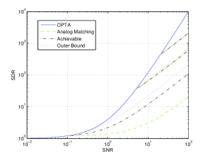
(a) $\rho=2$

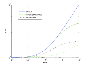
(b) $\rho=\frac{1}{2}$

Figure 9: *

Figure 9: Unknown SNR performance: BW expansion and compression. The best known achievable performance, brought for comparison, is due to [18, 24].

Comparison of performance: In comparison, the performance reported by different methods in [18, 24] for these cases has, in terms of (46):

$$\Phi_{\rho}({\text{SNR}},{\text{SNR}}_{0})=(1+{\text{SNR}})\cdot(1+{\text{SNR}}_{0})^{\rho-1}-1\ \,$$ (48)

while [24] also proves an outer bound for BW expansion ($\rho>1$) on any scheme which is optimal at some SNR:

$$\Phi_{\rho}({\text{SNR}},{\text{SNR}}_{0})=\frac{{\text{SNR}}}{{\text{SNR}}_{0}}\Bigl{[}(1+{\text{SNR}}_{0})^{\rho}-1\Bigr{]}\ \ .$$ (49)

In both BW expansion and compression, the Analog Matching scheme does not perform as good as the previously reported schemes, although the difference vanishes for high SNR. The basic drawback of analog matching compared to methods developed specifically for these special cases seems to be, that these methods apply different “zooming” to different source or channel frequency bands, analog matching uses the same “zooming factor” $\beta$ for all bands. Enhancements to the scheme, such as the combination of analog matching with pure analog transmission, may improve these results. Figure 9 demonstrates these results, for systems which are optimal at different SNR levels.

At high SNR, the performance of all these methods and of the outer bound converge to:

$$\frac{1}{{\text{SDR}}}=\frac{1-\min(\rho,1)}{{\text{SNR}}_{0}^{\rho}}+\frac{\min(\rho,1)}{{\text{SNR}}\cdot{\text{SNR}}_{0}^{\rho-1}}\ \ .$$ (50)

Thus the Analog Matching scheme, as well as the schemes of [18, 24], are all asymptotically optimal for high SNR among the schemes which achieve ${\text{SDR}}^{opt}$ at some SNR.

IV-D Asymptotic Behavior with BW Change

Finally we turn back to the general case of non-white spectra with any $\rho$, and examine it in the high-SNR regime. As in Section IV-B, we assume that the channel ISI filter is known, corresponding with an equivalent noise spectrum $S_{Z}({e^{j2\pi f}})$ known up to a scalar factor.

In the high-SNR limit, Lemma 3 implies:

$$\frac{1}{{\text{SDR}}}=\left[\frac{1-\min(\rho,1)}{{\text{SNR}}_{0}^{\rho}}+\frac{\min(\rho,1)}{{\text{SNR}}\cdot{\text{SNR}}_{0}^{\rho-1}}\right]\Gamma_{C}\Gamma_{S}\ \ .$$ (51)

Comparing with (50), we see that the color of the source and of the noise determines a constant factor by which the SDR is multiplied, but the dependence upon the SNR remains similar to the white BW expansion/compression case. The following definition formalizes this behavior (see [16]).

Definition 4

The distortion slope of a continuum of SNR-dependent schemes is :

$$\lambda\stackrel{{\scriptstyle\Delta}}{{=}}\lim_{{\text{SNR}}\rightarrow\infty}\frac{\log{\text{SDR}}}{\log{\text{SNR}}}\$$ (52)

where SDR is the signal to distortion attained at signal to noise ratio SNR, where the limit is taken for a fixed channel filter with noise variance approaching $0$.

We use the notation $\lambda=\lambda(\rho)$ in order to emphasize the dependance of the asymptotic slope upon the bandwidth expansion factor. The following follows directly from Proposition 1.

Proposition 3

For any source and channel spectra with BW ratio $\rho$, and for a continuum of schemes achieving the OPTA performance (17),

$$\lambda(\rho)=\rho\ \ .$$

As for an analog matching scheme which is optimal for a single SNR, (51) implies:

Corollary 2

For any source and channel spectra and for a single analog-matching encoder,

$$\lambda(\rho)=\left\{\begin{array}[]{lll}1,&\mbox{if $\rho\geq 1$}\\ 0,&\mbox{otherwise}\end{array}\right\}$$

is achievable.

This asymptotic slope agrees with the outer bound of [24] for the (white) bandwidth expansion problem. For the bandwidth compression problem, no outer bound is known, but we are not aware of any proposed scheme with a non-zero asymptotic slope. We believe this to be true for all spectra:

Conjucture 1

For any source and channel spectra of BW ratio $\rho$, no single encoder which satisfies (17) at some ${\text{SNR}}_{0}$ can have a better slope than that of Corollary 2.

By this conjecture, the analog matching encoder is asymptotically optimal among all encoders ideally matched to one SNR. It should be noted, that schemes which do not satisfy optimality at one SNR can in fact approach the ideal slope $\lambda(\rho)=\rho$. See e.g. approaches for integer $\rho$ such as bit interleaving [26].

V Conclusion: Implementation and Applications

We presented the Analog Matching scheme, which optimally transmits a Gaussian source of any spectrum over a Gaussian channel of any spectrum, without resorting to any data-bearing code. We showed the advantage of such a scheme over a separation-based solution, in the sense of robustness for unknown channel SNR.

The analysis we provided was asymptotic, in the sense that a high-dimensional lattice is needed. However, unlike digital transmission (and hybrid digital-analog schemes) where reduction of the code block length has a severe impact on performance, the semi-analog approach offers a potential advantage in terms of block-length. An asymptotic figure of merit where we expect this advantage to be revealed, is the excess-distortion exponent. Furthermore, the modulo-lattice framework allows in practice reduction to low-dimensional, even scalar lattices, with bounded loss.

One approach for scalar implementation of the Analog Matching scheme, uses companding [17]. In this approach, the scalar zooming factor $\beta$ is replaced by a non-linear function which compresses the unbounded Gaussian source into a finite range, an operation which is reverted at the decoder. There is a problem here, since the entity which needs to be compressed is actually the innovations process $\tilde{Q}_{n}$, unknown at the encoder since it depends on the channel noise. This can be solved by compressing $Q_{n}$, the innovations of the source itself; The effect of this “companding encoder-decoder mismatch” vanishes in the high-SNR limit. An altogether different approach, is to avoid instantaneous decoding of the lattice; Instead, the decoder may at each instance calculate the source prediction using several hypothesis in parallel. The ambiguity will be solved in future instances, possibly by a trellis-like algorithm.

In terms of delay, the AM scheme has an additional advantage over previously suggested HDA schemes. It is well known that time-domain approaches have a delay advantage over frequency-domain one, in both source and channel coding. A fully-causal DPCM, for example, can approach the RDF while only using causal filters, on the high-resolution limit. A sub-band coding scheme, in contrast, would have to use a delay-consuming DFT block; see e.g. [13].

Finally, we remark that the AM scheme has further applications. It possesses the basic property, that it converts any colored channel to an equivalent additive white noise channel of the same capacity as the original channel, but of the source bandwidth. In the limit of high-SNR, this equivalent noise becomes Gaussian and independent of any encoder signal. This property is plausible in multi-user source, channel and joint source/channel problems, in the presence of bandwidth mismatch. Applications include computation over MACs [21], multi-sensor detection [20] and transmission over the parallel relay network [14].

-A Proof of Proposition 2

By [8, (200)], for each of the components $Z_{l}$:

$$\frac{1}{n}\log\frac{f_{Z_{l}}(z)}{f_{Z^{\prime}_{l}(z)}}\leq\epsilon(\Lambda_{K})$$ (53)

where $f(\cdot)$ denotes a probability density function (pdf), $Z^{\prime}_{l}$ is AWGN with the same variance as $Z_{l}$, and $\epsilon(\Lambda_{K})\rightarrow 0$ as $K\rightarrow\infty$ for a sequence of lattices which is Rogers-good (i.e. lattices for which volume of the covering sphere approaches that of the Voronoi cell). Now assume without loss of generality that $\alpha_{l}^{2}$ is a non-increasing for $l>0$, and for some fixed $\delta$ let $L^{\prime}$ be the minimal index such that

$$\sum_{l=L^{\prime}+1}^{\infty}\alpha_{l}^{2}\leq\delta\ \ .$$

Let $Z_{\delta}=\sum_{l=1}^{L^{\prime}}\alpha_{l}Z_{l}$. Using (53) and convolution of pdfs,

$$\frac{1}{n}\log\frac{f_{Z_{\delta}}(z)}{f_{Z^{\prime}_{\delta}(z)}}\leq\epsilon^{L^{\prime}}(\Lambda_{K})\ \ ,$$

where $Z^{\prime}_{\delta}$ is AWGN with the same variance as $Z_{\delta}$. Since $\epsilon^{L^{\prime}}$ approaches zero as a function of $K$,

$$\lim_{K\rightarrow\infty}\Pr\{Z_{0}+Z_{\delta}\notin{\mathcal{V}}_{K}\}=0\ \ ,$$

for lattices which are good for AWGN coding.

We are left with the “tail” $\tilde{Z}=\sum_{l=L^{\prime}+1}^{\infty}\alpha_{l}Z_{l}$, which has variance $\delta$. By continuity arguments,

$$\lim_{\delta\rightarrow 0^{+}}\Pr\{Z_{0}+Z_{\delta}+\tilde{Z}\notin{\mathcal{V}}_{K}|Z_{0}+Z_{\delta}\in{\mathcal{V}}_{K}\}=0\ \ .$$

The result follows now by standard arguments of taking $\epsilon$ and $\delta$ to zero simultaneously. We have assumed the use of a sequence of lattices that is simultaneously Rogers-good and AWGN-good. By [7], such a sequence indeed exists.

-B Proof of Lemma 1

By the properties of the modulo-lattice operation, $\tilde{X}_{n}$ is a white process. Now the channel from $\tilde{X}_{n}$ to $\tilde{Y}_{n}$ is identical to the channel of (25), thus we have that:

$$Y^{\prime}_{n}=(\tilde{X}_{n}+\tilde{Z}_{n})*(\delta_{n}-{p_{C}}_{n})=\tilde{X}_{n}+I_{n}+Z^{\prime\prime}_{n}\ \ ,$$

where $\tilde{Z}_{n}$ has spectrum $S_{\tilde{Z}}({e^{j2\pi f}})$ (33), and consequently $Z^{\prime\prime}_{n}=\tilde{Z}_{n}*(\delta_{n}-{p_{C}}_{n})$ is its white prediction error, with variance $\frac{1-\alpha}{\alpha}\theta_{C}$ according to (27). Now since $\tilde{Y}_{n}=Y^{\prime}_{n}-I_{n}$ is the optimum linear estimator for $\tilde{X}_{n}$ from the channel output, the orthogonality principle dictates that the estimation error is uncorrelated with the process $Y^{\prime}_{n}$, resulting in an additive backward channel (see e.g. [35]):

$$\tilde{X}_{n}=Y^{\prime}_{n}-I_{n}+Z^{\prime\prime}_{n}\ \ .$$

Switching back to a forward channel, we have

$$Y^{\prime}_{n}=\alpha(\tilde{X}_{n}+Z^{\prime}_{n})+I_{n}\ \ ,$$

where $Z^{\prime}_{n}$ is white with the same variance as $Z^{\prime\prime}_{n}$. Furthermore, since $Z^{\prime}_{n}$ is a function of the processes $\{\tilde{X}_{n}\}$ and $\{Z_{n}\}$, it is independent of all $U_{n}$.

-C Proof of Lemma 2

By the properties of the modulo-lattice operation,

$$T_{n}=\beta(U_{n}-J_{n})+{Z_{eq}}_{n}\ \ ,$$

resulting in the equivalent channel of Figure 8b. By the correct initialization assumption, (39) holds for all past instances, thus ${\bf T}_{n}$ is a combination noise (see Definition 2). In light of Proposition 2, it is only left to show that the variance of $T_{n}$ is strictly less than the lattice second moment $\theta_{C}$. To that end, note that under the correct initialization assumption, the past samples of the process $V_{n}$ indeed behave as samples of a stationary process of spectrum $S_{V}({e^{j2\pi f}})$ (32), for which $P_{S}({e^{j2\pi f}})$ is the optimal predictor. It follows that $U_{n}-J_{n}$ is white, with variance

$$\mathop{\mathrm{Var}}\{U_{n}-J_{n}\} = \mathop{\mathrm{Var}}\{U_{n}|V_{n-1},V_{n-2},\ldots\}$$

$$\stackrel{{\scriptstyle(a)}}{{=}} P_{e}\Bigl{(}S_{U}+\frac{\mathop{\mathrm{Var}}\{{Z_{eq}}_{n}\}}{\beta^{2}}\Bigr{)}-\frac{\mathop{\mathrm{Var}}\{{Z_{eq}}_{n}\}}{\beta^{2}}$$

$$= P_{e}\Bigl{(}S_{U}+\frac{\beta_{0}^{2}}{\beta^{2}}\theta_{S}\Bigr{)}-\frac{\beta_{0}^{2}}{\beta^{2}}\theta_{S}$$

$$< \frac{\beta_{0}^{2}}{\beta^{2}}\Bigl{[}P_{e}(S_{U}+\theta_{S})-\theta_{S}\Bigr{]}$$

$$\stackrel{{\scriptstyle(b)}}{{=}} \frac{\beta_{0}^{2}}{\beta^{2}}\cdot\frac{\alpha}{1-\alpha}\theta_{S}$$

$$= \frac{\alpha\theta_{C}}{\beta^{2}}\ \ ,$$

where $(a)$ holds by (10), and $(b)$ holds by applying the same in the opposite direction, combined with (23). By the whiteness of ${Z_{eq}}_{n}$ and its independence of all $U_{n}$, we have that $U_{n}-J_{n}$ is independent of ${Z_{eq}}_{n}$, thus the variance of $T_{n}$ is given by

$$\mathop{\mathrm{Var}}\{T_{n}\}=\beta^{2}\mathop{\mathrm{Var}}\{U_{n}-J_{n}\}+\mathop{\mathrm{Var}}\{{Z_{eq}}_{n}\}<\theta_{C}\ \ .$$ (54)

The margin from $\theta_{C}$ depends on the margin in the inequality in the chain above, which depends only on $S_{U}({e^{j2\pi f}})$, $\theta_{C}$ and $\beta$, and is strictly positive for all $\beta<\beta_{0}$.

-D Proof of Lemma 3

We work with the optimum Analog Matching encoder for the noise spectrum $S_{Z0}({e^{j2\pi f}})$. At the decoder, we note that for any choice of the channel post-filter $G_{2}({e^{j2\pi f}})$, we have that the equivalent noise ${{Z_{eq}}_{n}}$ is the noise ${{\tilde{Z}}_{n}}\stackrel{{\scriptstyle\Delta}}{{=}}{{\tilde{Y}}_{n}}-{{\tilde{X}}_{n}}$ passed through the filter $1-P_{C}({e^{j2\pi f}})$. Consequently, this noise has spectrum:

$$S_{eq}({e^{j2\pi f}})=S_{\tilde{Z}}({e^{j2\pi f}})|1-P_{C}({e^{j2\pi f}})|^{2}\ \ .$$

The filter $G_{2}({e^{j2\pi f}})$ should, therefore, be the Wiener filter which minimizes $S_{\tilde{Z}}({e^{j2\pi f}})$ at each frequency. This filter achieves a noise spectrum

$$S_{\tilde{Z}}({e^{j2\pi f}})=\frac{\theta_{C}-S_{Z0}({e^{j2\pi f}})}{\theta_{C}-S_{Z0}({e^{j2\pi f}})+S_{Z}({e^{j2\pi f}})}S_{Z}({e^{j2\pi f}})$$

inside ${\cal F}_{C}$, and $\theta_{C}$ outside. Denoting the variance of the (white) equivalent noise in the case $S_{Z0}({e^{j2\pi f}})=S_{Z}({e^{j2\pi f}})$ as $S_{0}=(1-\alpha)\theta_{C}$ (41), we find that:

$$|1-P_{C}({e^{j2\pi f}})|^{2}=\frac{S_{0}\theta_{C}}{(\theta_{C}-S_{Z0}({e^{j2\pi f}}))S_{Z0}({e^{j2\pi f}})}$$

inside ${\cal F}_{C}$, and $S_{0}/\theta_{C}$ outside. We conclude that we have equivalent channel noise with spectrum

$$S_{eq}({e^{j2\pi f}})=\frac{S_{Z}({e^{j2\pi f}})}{S_{Z0}({e^{j2\pi f}})}\cdot\frac{\theta_{C}}{\theta_{C}-S_{Z0}({e^{j2\pi f}})+S_{Z}({e^{j2\pi f}})}S_{0}=\frac{S_{S}({e^{j2\pi f}})-\theta_{S}}{\Phi({e^{j2\pi f}})\theta_{S}}S_{0}$$ (55)

inside ${\cal F}_{C}$, and $S_{0}$ outside. Now, since this spectrum is everywhere upper-bounded by $S_{0}$, we need not worry about correct decoding. The source post-filter input is the source, corrupted by an additive noise ${Z_{eq}}_{n}/\beta$, with spectrum arbitrarily close to

$$\frac{S_{eq}({e^{j2\pi f}})}{\beta_{0}^{2}}=\frac{S_{S}({e^{j2\pi f}})-\theta_{S}}{\Phi({e^{j2\pi f}})}\ \$$

inside ${\cal F}_{C}$, and $\theta_{S}$ outside. Now again we face optimal linear filtering, and we replace the source post-filter $F_{2}({e^{j2\pi f}})$ by the Wiener filter for the source, to arrive at the desired result.

References

- [1] T. Berger and D.W. Tufts. Optimum pulse amplitude modulation part I: Transmitter-receiver design and bounds from information theory. IEEE Trans. Info. Theory, IT-13:196–208, Apr. 1967.
- [2] B. Chen and G. Wornell. Analog error-correcting codes based on chaotic dynamical systems. IEEE Trans. Communications, 46:881–890, July 1998.
- [3] J.M. Cioffi, G.P. Dudevoir, M.V. Eyuboglu, and G.D. J. Forney. MMSE decision-feedback equalizers and coding - Part I: Equalization results. IEEE Trans. Communications, COM-43:2582–2594, Oct. 1995.
- [4] M.H.M. Costa. Writing on dirty paper. IEEE Trans. Info. Theory, IT-29:439–441, May 1983.
- [5] L. W. Couch. Digital & Analog Communication Systems (7th Edition). Prentice Hall, 2006.
- [6] T. M. Cover and J. A. Thomas. Elements of Information Theory. Wiley, New York, 1991.
- [7] U. Erez, S. Litsyn, and R. Zamir. Lattices which are good for (almost) everything. IEEE Trans. Info. Theory, IT-51:3401–3416, Oct. 2005.
- [8] U. Erez and R. Zamir. Achieving 1/2 log(1+SNR) on the AWGN channel with lattice encoding and decoding. IEEE Trans. Info. Theory, IT-50:2293–2314, Oct. 2004.
- [9] G. D. Forney, Jr. Shannon meets Wiener II: On MMSE estimation in successive decoding schemes. In 42nd Annual Allerton Conference on Communication, Control, and Computing, Allerton House, Monticello, Illinois, Oct. 2004.
- [10] M. Gastpar, B. Rimoldi, and M. Vetterli. To code or not to code: Lossy source-channel communication revisited. IEEE Trans. Info. Theory, IT-49:1147–1158, May 2003.
- [11] T.J. Goblick. Theoretical limitations on the transmission of data from analog sources. IEEE Trans. Info. Theory, IT-11:558–567, 1965.
- [12] T. Guess and M. Varanasi. An information-theoretic framework for deriving canonical decision-feedback receivers in Gaussian channels. IEEE Trans. Info. Theory, IT-51:173–187, Jan. 2005.
- [13] N. S. Jayant and P. Noll. Digital Coding of Waveforms. Prentice-Hall, Englewood Cliffs, NJ, 1984.
- [14] Y. Kochman, A. Khina, U. Erez, and R. Zamir. Rematch and forward for parallel relay networks. In ISIT-2008, Toronto, ON, pages 767–771, 2008.
- [15] Y. Kochman and R. Zamir. Joint Wyner-Ziv/dirty-paper coding by modulo-lattice modulation. IEEE Trans. Info. Theory, IT-55:4878–4899, Nov. 2009.
- [16] J.N. Laneman, E. Martinian, G.W. Wornell, and J.G. Apostolopoulos. Source-channel diversity approaches for multimedia communication. IEEE Trans. Info. Theory, IT-51:3518–3539, Oct. 2005.
- [17] I. Leibowitz. The Ziv-Zakai bound at high fidelity, analog matching, and companding. Master’s thesis, Tel Aviv University, Nov. 2007.
- [18] U. Mittal and N. Phamdo. Hybrid digital-analog (HDA) joint source-channel codes for broadcasting and robust communications. IEEE Trans. Info. Theory, IT-48:1082–1103, May 2002.
- [19] K. Narayanan, M. P. Wilson, and G. Caire. Hybrid digital and analog Costa coding and broadcasting with bandwidth compression. Technical Report 06-107, Texas A&M University, College Station, August 2006.
- [20] B. Nazer and M. Gastpar. Compute-and-forward: Harnessing interference with structured codes. In ISIT-2008, Toronto, ON, pages 772–776, 2008.
- [21] B. Nazer and M. Gastpar. Computation over multiple-access channels. IEEE Trans. Info. Theory, IT-53:3498–3516, Oct. 2007.
- [22] V. M. Prabhakaran, R. Puri, and K. Ramchandran. A hybrid analog-digital framework for source-channel broadcast. In Proceedings of the 43rd Annual Allerton Conference on Communication, Control and Computing, 2005.
- [23] R. Puri and K. Ramchandran. PRISM: A ’reversed’ multimedia coding paradigm. In Proc. IEEE Int. Conf. Image Processing, Barcelona, 2003.
- [24] Z. Reznic, M. Feder, and R. Zamir. Distortion bounds for broadcasting with bandwidth expansion. IEEE Trans. Info. Theory, IT-52:3778–3788, Aug. 2006.
- [25] S. Shamai, S. Verdú, and R. Zamir. Systematic Lossy Source/Channel Coding. IEEE Trans. Info. Theory, 44:564–579, March 1998.
- [26] M. Taherzadeh and A. K. Khandani. Robust joint source-channel coding for delay-limited applications. In ISIT-2007, Nice, France, pages 726–730, 2007.
- [27] M. Tomlinson. New automatic equalizer employing modulo arithmetic. Elect. Letters, 7:138–139, March 1971.
- [28] H. L. Van Trees. Detection, Estimation, and Modulation theory. Wiley, New York, 1968.
- [29] M. D. Trott. Unequal error protection codes: Theory and practice. In Proc. of Info. Th. Workshop, Haifa, Israel, page 11, June 1996.
- [30] V.A. Vaishampayan and S.I.R. Costa. Curves on a sphere, shift-map dynamics, and error control for continuous alphabet sources. IEEE Trans. Info. Theory, IT-49:1658–1672, July 2003.
- [31] M.P Wilson, K. Narayanan, and G. Caire. Joint source chennal coding with side information using hybrid digital analog codes. In Proceedings of the Information Theory Workshop, Lake Tahoe, CA, pages 299–308, Sep. 2007.
- [32] A.D. Wyner and J. Ziv. The rate-distortion function for source coding with side information at the decoder. IEEE Trans. Info. Theory, IT-22:1–10, Jan., 1976.
- [33] R. Zamir and M. Feder. On lattice quantization noise. IEEE Trans. Info. Theory, pages 1152–1159, July 1996.
- [34] R. Zamir and M. Feder. Information rates of pre/post filtered dithered quantizers. IEEE Trans. Info. Theory, pages 1340–1353, Sep. 1996.
- [35] R. Zamir, Y. Kochman, and U. Erez. Achieving the Gaussian rate distortion function by prediction. IEEE Trans. Info. Theory, IT-54:3354–3364, July 2008.
- [36] R. Zamir, S. Shamai, and U. Erez. Nested linear/lattice codes for structured multiterminal binning. IEEE Trans. Info. Theory, IT-48:1250–1276, June 2002.
- [37] J. Ziv. The behavior of analog communication systems. IEEE Trans. Info. Theory, IT-16:587–594, 1970.