Probing Dark Energy with the Kunlun Dark Universe Survey Telescope

Abstract

Dark energy is an important science driver of many upcoming large-scale surveys. With small, stable seeing and low thermal infrared background, Dome A, Antarctica, offers a unique opportunity for shedding light on fundamental questions about the universe. We show that a deep, high-resolution imaging survey of 10,000 square degrees in ugrizyJH bands can provide competitive constraints on dark energy equation of state parameters using type Ia supernovae, baryon acoustic oscillations, and weak lensing techniques. Such a survey may be partially achieved with a coordinated effort of the Kunlun Dark Universe Survey Telescope (KDUST) in yJH bands over 5000–10,000 deg² and the Large Synoptic Survey Telescope in ugrizy bands over the same area. Moreover, the joint survey can take advantage of the high-resolution imaging at Dome A to further tighten the constraints on dark energy and to measure dark matter properties with strong lensing as well as galaxy–galaxy weak lensing.

1. Introduction

Antarctic Plateau, especially the Kunlun Station under construction by the Polar Research Institute of China (PRIC), provides a unique opportunity for wide field astronomical surveys targeting cosmological studies. Astronomical site survey of Dome A, Antarctica was enabled by the International Polar Year (IPY) endorsed PANDA program (Yang et al. 2009) led by the PRIC and the Chinese Center for Antarctica Astronomy (CCAA). Several international teams contributed to this effort. In particular, the power and on-site laboratory system built by the University of New South Wales (BUN’S) has provided the platform for all the site survey instruments.

In its two years’ operation, the site survey effort proves practically all aspects of the theoretical expectations of the Dome A site for astronomical observations. Preliminary analyses show that the boundary layer of atmospheric turbulence to be around $10-20$ meters during the Antarctic winter (Ashley et al. 2010). Similar to the relatively better studied neighboring Dome C site (Fossat et al. 2010), the Dome A site may enjoy free atmospheric seeing conditions of about 0.3 arcsec seeing above this boundary layer, thus making it an ideal site for high angular resolution wide area surveys.

The temperature at Dome A is around $-60$ to $-70\degree{C}$, making it the coldest spot on the surface of the Earth. This implies a very low thermal background emission in the thermal infrared. The Dome A site is thus also the best site for astronomical observations in the near infrared wavelength region.

One other especially exciting property of the site is the lack of water vapors due to the high altitude and the low temperature. This implies that the site is also ideal for terahertz observations which have been impossible from any temperate sites on Earth.

While quantitative site properties are still under analyses and longer term monitoring are still needed to firmly establish the astronomical potential of the Dome A site, there is no doubt that a survey project at Dome A can be highly complimentary to programs such as the Large Synoptic Survey Telescope (LSST, LSST Science Collaborations 2009), the Joint Dark Energy Mission, and Euclid. For example, a survey at Dome A can provide near infrared data that compliments the deep optical band survey of the LSST; a deep survey in the near infrared combined with the optical data from LSST can reveal high redshift objects at $z\sim 10$, which are not detectable in the optical. The Kunlun Dark Universe Survey Telescope (KDUST) is a 6-to-8-meter wide-area survey telescope being designed by the CCAA. The preliminary design includes a $3\times 3$ square degree optical camera with $0^{\prime\prime}.15$ pixel, and an infrared camera of $1\times 1$ square degree at $0^{\prime\prime}.1$/pixel optimized for $1-3.5$ $\mu$m surveys.

One of the key science missions of KDUST is to investigate the mystery of the accelerated cosmic expansion (Riess et al. 1998; Perlmutter et al. 1999) using multiple techniques. In this paper, we estimate how well an ideal 10,000 deg² ugrizyJH survey can constrain the dark energy equation of state (EOS) with weak lensing (WL), baryon acoustic oscillations (BAOs), and type Ia supernova (SNe) luminosity distances. These dark energy probes have different sensitivities to the cosmic expansion and structure growth as well as various systematic uncertainties in the observations, and hence are highly complementary to each other for constraining dark energy properties (e.g., Knox et al. 2005; Zhan 2006; Zhan et al. 2009).

The SNe technique relies on the standardizable candle of the SNe intrinsic luminosity (Phillips 1993) to measure the luminosity distance, $D_{\rm L}(z)$. Dark energy properties can then be inferred from the distance–redshift relation. The BAO technique utilizes the standard ruler of the baryon imprint on the matter (and hence galaxy) power spectrum (Peebles & Yu 1970; Bond & Efstathiou 1984) to measure the angular diameter distance, $D_{\rm A}(z)$, and, if the redshifts are sufficiently accurate, the Hubble parameter, $H(z)$ (Eisenstein et al. 1998; Cooray et al. 2001; Blake & Glazebrook 2003; Hu & Haiman 2003; Linder 2003; Seo & Eisenstein 2003). The WL technique has the advantage that it can measure both $D_{\rm A}(z)$ from the lensing kernel and the growth factor of the large-scale structure $G(z)$ (Hu & Tegmark 1999; Huterer 2002; Refregier 2003; Takada & Jain 2004; Knox et al. 2006a; Zhan et al. 2009).

Because of the excellent seeing condition and infrared accessibility at Dome A, KDUST has a number of advantages for the commonly used cosmological probes. For example, the signal-to-noise ratio for point sources is inversely proportional to the seeing. Thus, a 6 meter telescope at Dome A ($\sim 0^{\prime\prime}.3$ median seeing in the optical) would be equivalent to a 14 meter telescope at a temperate site ($\sim 0^{\prime\prime}.7$ seeing) for point-source observations with the same sky background level. An 8m KDUST could detect SNe out to redshift 3 in the $K_{\rm dark}$ ($2.27$–$2.45\mu$m, redward of $K$) band (Kim et al. 2010). Although high-z distances are not sensitive to conventional dark energy, they can be used to determine the mean curvature accurately, which, in turn, helps constrain dark energy EOS (Linder 2005; Knox et al. 2006b). Moreover, even though dark energy is thought to be sub-dominant at high redshift, there is no direct evidence to prove one way or another. Measurements of SNe at $z>2$ will provide crucial data for tests of early dark energy.

Small and stable seeing is particularly helpful for WL. One could resolve more galaxies at the same surface brightness limit, which reduces the shape noise for shear measurements. Fine resolution helps measure the shape accurately and reduce the shear measurement systematic errors. In addition, deep JH photometry can track the 4000Å break of an elliptical galaxy to $z\sim 3$ and improve photometric redshifts (photo-zs) as well as systematic uncertainties in the photo-z error distribution (Abdalla et al. 2008), which has a large impact on WL constraints on the dark energy EOS (Huterer et al. 2006; Ma et al. 2006; Zhan 2006).

Adding K or $K_{\rm dark}$ band will certainly improve galaxy photo-zs, especially at $z\gtrsim 3$. However, currently planned multiband dark energy surveys use galaxies at $z\lesssim 3$, and their concern is the confusion between $z\lesssim 0.5$ ellipticals and $2\lesssim z\lesssim 3.5$ star-forming galaxies, which is greatly mitigated by $u$ and $JH$ bands (Abdalla et al. 2008). Another consideration is that Dome A is far more advantageous at $K_{\rm dark}$ band than at $K$ band because of the low thermal background there, so $K_{\rm dark}$ is likely to be chosen over $K$. This would leave a considerable gap in the wavelength coverage and reduce the already-small gain on photo-zs in the useful redshift range for dark energy investigations. Therefore, we do not discuss utilities of wavebands beyond $H$ in this paper. Nevertheless, the $K_{\rm dark}$ band is crucial for a broad range of other sciences and will be an important aspect of the KDUST survey.

This paper is organized as follows. Section 2 discusses the survey plan of KDUST including that of its pathfinder in context of the LSST survey. We then consider a joint KDUST and LSST survey in section 3 for constraining the dark energy EOS with BAO, WL, and type Ia SN techniques. The results are presented in both two-parameter space where the dark energy EOS is parameterized as $w(z)=w_{0}+w_{a}z(1+z)^{-1}$ and in model-independent principle component space. The conclusion is drawn in section 4.

2. A Potential KDUST Survey Plan

Dome A has a great potential for cosmology, but, given other ambitious projects that will be concurrent with KDUST, one must carefully plan the KDUST survey to make the best use of the Dome A site. As we discuss, below, a potentially efficient strategy for KDUST is to focus on the near infrared (NIR) bands and incorporate optical data from LSST or other surveys.

In the optical bands, a 6m KDUST is about twice as fast as LSST for surveying sky-dominated point sources at the same sky level, in which case the survey speed is proportional to the aperture and field of view and inversely proportional to the seeing disk area. In reality, aurorae increase the sky brightness in short wavelengths. It is estimated that the sky brightness at Dome A would be twice as bright as that at the best temperate site in $B$ and 20%–30% brighter in $V$ (Saunders et al. 2009); measurements have shown that the median $i$-band sky brightness at Dome A in 2008 was $19.81$ mag arcsec^-2 and $20.46$ mag arcsec^-2 during dark time, better than that at other good sites (Zou et al. 2010). With the above considerations, the 6m KDUST could survey 10,000 deg² to LSST depths in $griz$ and much deeper in $y$ ($\sim 26$ mag, $5\sigma$ point sources) in 2.5 years. The NIR camera of KDUST would have a much smaller field of view. It could reach $J=25$ mag and $H=24.6$ mag over the same area in 3.5 years.

Since LSST plans to survey the southern sky in $ugrizy$, it is not absolutely necessary for KDUST to survey in the optical again except in the $y$ band. LSST would spend 20% of its time in $y$ band to achieve a 5-$\sigma$ limiting magnitude of 24.4 for point sources, which is 2.8 magnitudes shallower than its $r$ band limit. From photo-z consideration, it is desirable to have the $y$ band limit not too much shallower than the limits in shorter wavebands. KDUST could improve the situation in its 10,000 deg² survey area, which would be covered by LSST as well. A joint effort of KDUST in $yJH$ and LSST in $ugrizy$ would save both projects time while achieving better performance in measuring the dark energy EOS.

Here, we use SNAP and LSST as references to model an ideal 10,000 square degree survey (named “ideal 10k”) in ugrizyJH bands to comparable depth as SNAP. We assume that its galaxy redshift distribution follows

$$n(z)\propto z^{2}e^{-z/z_{*}}$$

with $z_{*}=0.5$. The projected galaxy number density $\bar{n}_{g}$ is 70 arcmin^-2, and the distribution peaks at $2z_{*}$. For LSST, we adopt $z_{*}=0.3$ and $\bar{n}_{g}=40$ arcmin^-2 (LSST Science Collaborations 2009). The model parameters of the survey data are summarized in Table 1.

The galaxy distribution $n_{i}(z)$ in the $i$th bin is sampled from $n(z)$ by (Ma et al. 2006; Zhan 2006)

$$n_{i}(z)=n(z)\mathcal{P}(z_{{p},i}^{\rm B},z_{{p},i}^{\rm E};z),$$

where the subscript p denotes photo-z space, $z_{{p},i}^{\rm B}$ and $z_{{p},i}^{\rm E}$ define the extent of bin $i$, and $\mathcal{P}(a,b;z)$ is the probability of assigning a galaxy that is at true redshift $z$ to the photo-z bin between $z_{p}=a$ and $b$. We approximate the photo-z error to be Gaussian with bias $\delta z$ and rms $\sigma_{z}=\sigma_{z0}(1+z)$, and the probability becomes

$$\mathcal{P}(z_{{p},i}^{\rm B},z_{{p},i}^{\rm E};z) = I(z_{{p},i}^{\rm B},z_{{p},i}^{\rm E};z)/I(0,\infty;z),$$

$$I(a,b;z) = \frac{1}{\sqrt{2\pi}\,\sigma_{z}}\int_{a}^{b}dz_{p}\,\exp\left[-\frac{(z_{p}-z-\delta z)^{2}}{2\sigma_{z}^{2}}\right].$$

The normalization $I(0,\infty;z)$ implies that galaxies with a negative photo-z have been excluded from $n(z)$. We use 40 photo-z bias $\delta z$ and 40 photo-z rms $\sigma_{z}$ parameters evenly spaced between $z=0$ and 5 to model the photo-z error distribution in the $z$–$z_{p}$ space; the photo-z bias and rms at any redshift are linearly interpolated from these 80 parameters. Note that the photo-z parameters are assigned independent of galaxy bins. We assume that $\sigma_{z0}=0.03$ for the ideal survey and $\sigma_{z0}=0.05$ for LSST.

Table 1Model parameters of survey data and priors.

	Ideal 10k	LSST	KDUST+LSST
area (deg2)	10,000	20,000	10,000 + 10,000
$n_{\rm g}$ (arcmin-2)	70	40	60	40
$z_{*}$	0.5	0.3	0.4	0.3
$\sigma_{z0}$	0.03	0.05	0.03	0.04
$\sigma_{\rm P}(\delta z)$	$0.2\sigma_{z}$	$0.3\sigma_{z}$	$0.2\sigma_{z}$	$0.2\sigma_{z}$
$\sigma_{\rm P}(f^{\gamma}_{i})$	0.002	0.005	0.002	0.003
$(A_{i}^{\gamma})^{2}(\times 10^{-10})$	$4$	$10$	$4$	$6$

Uncertainties of the photo-z parameters (or, the photo-z error distribution in general) have a large impact on the dark energy constraints from WL and are referred to as photo-z systematics. Therefore, the prior on the photo-z error distribution is an important quantity to specify when reporting WL constraints on dark energy. To reduce the dimension of the investigation, we set a simple function for all the priors on the photo-z bias parameters, $\sigma_{\mathrm{P}}(\delta z)=0.2\sigma_{z}$, and peg the priors on photo-z rms parameters to those on the bias parameters: $\sigma_{\mathrm{P}}(\sigma_{z})=\sqrt{2}\sigma_{\mathrm{P}}(\delta z)$. For Gaussian photo-z errors, these priors correspond to a calibration sample of 25 spectra per redshift interval of the photo-z parameters. We set $\sigma_{\mathrm{P}}(\delta z)=0.3\sigma_{z}$, reflecting larger uncertainties with fewer filter bands. However, such difference in the photo-z priors is not important if one performs a joint analysis of the BAO and WL techniques, which takes advantage of the self-calibration of photo-z error distribution by galaxy power spectra (Schneider et al. 2006; Zhan 2006; Zhang et al. 2009, referenced herein)

LSST will benefit from KDUST $yJH$ data in a number of ways. In the 10,000 deg² overlap region, KDUST data will (1) improve photo-zs directly, (2) increase the galaxy sample with those that would not meet the LSST optical photometry selection criteria, or whose photo-z could not be reliably determined in the absence of the deep $yJH$ data, or whose shape could not be measured well because of the larger seeing at the LSST site, and (3) provide calibration of various systematic errors such as those in shear measurements. Even in the non-overlap region, LSST could still improve photo-zs and shear measurements because of the calibration within the overlap region. This is reflected in the last column of Table 1 where we construct a joint survey combining LSST and KDUST.

For the SN data, we assume that KDUST would obtain a SNAP-like sample of 2000 SNe reaching redshift $1.7$ as well as a sample of 1000 local and nearby SNe. Details of the assumptions for the SNAP experiments and the calculation of the Fisher matrices can be found in (Pogosian et al. 2005) and in (Zhao et al. 2009).

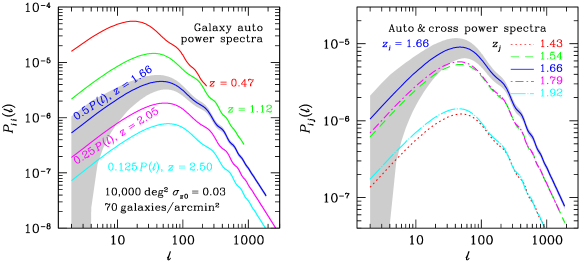
Figure 1.— Left panel: Five galaxy auto power spectra from the ideal 10k survey. The BAO feature is visible around $\ell\sim 400$ in the highest redshift bin and move toward lower multipoles in lower redshift bins. Note, however, that the linear scale of the BAOs is fixed in the comoving frame. The amplitude of the power spectra and that of the BAO feature decreases as the photo-z rms error increases. The shaded area gives the 1-$\sigma$ error (e.g., sample variance and shot noise) of the power spectrum per $\ell$ in the bin centered at $z=1.66$. The power spectra are shifted for clarity. Right panel: Cross power spectra between the bin at $z=1.66$ and its second neighboring bins and 4th neighboring bins.

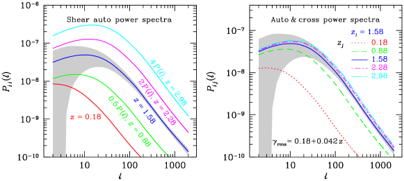
Figure 2.— Same as Figure 1 but for the shear power spectra in 5 different redshift bins. The shear power spectra are smoother than the galaxy power spectra, because lensing kernels are much broader that galaxy distributions in the photo-z bins.

3. Constraining Dark Energy with KDUST and LSST

In this section, we estimate the constraints on the dark energy EOS from the joint survey of KDUST and LSST using BAO, WL, and SN techniques.

3.1. Baryon Acoustic Oscillations and Weak Lensing

The angular power spectra of the galaxy number density $n(\bm{\theta})$ and (E-mode) shear $\gamma(\bm{\theta})$ can be written as (Hu & Jain 2004; Zhan 2006)

$$P_{ij}^{XY}(\ell)=\frac{2\pi^{2}}{c\ell^{3}}\int dz\,H(z)D_{\rm A}(z)W_{i}^{X}(z)W_{j}^{Y}(z)\Delta^{2}_{\delta}(k;z),$$ (1)

where lower case subscripts correspond to the tomographic bins, upper case superscripts label the observables, e.g., $X=\mbox{g}$ for galaxies or $\gamma$ for shear, $\Delta^{2}_{\delta}(k;z)$ is the dimensionless power spectrum of the density field, and $k=\ell/D_{\rm A}(z)$. The window functions are

$$W_{i}^{\rm g}(z) = b(z)\frac{n_{i}(z)}{\bar{n}_{i}},$$

$$W_{i}^{\gamma}(z) = \frac{3}{2}\frac{\Omega_{\rm m}H_{0}^{2}}{H(z)}\frac{D_{\rm A}(z)}{a\,c}\int_{z}^{\infty}\!dz^{\prime}\,\frac{n_{i}(z^{\prime})}{\bar{n}_{i}}\frac{D_{\rm A}(z,z^{\prime})}{D_{\rm A}(z^{\prime})},$$

where $b(z)$ is the linear galaxy clustering bias, and $\Omega_{\rm m}$ and $H_{0}$ are, respectively, the matter fraction at $z=0$ and Hubble constant. The galaxy redshift distribution $n_{i}(z)$ in the $i$th tomographic bin is an average of the underlying three-dimensional galaxy distribution over angles, and the mean surface density $\bar{n}_{i}$ is the total number of galaxies per steradian in bin $i$. For WL, we use 10 bins evenly spaced between $z=0$ to 3.5, and for BAO, we use 30 bins from $z=0.15$ to 3.5 with bin width proportional to $1+z$.

The $1\sigma$ statistical error of the mean power spectrum in the multipole range $(\ell,\ell+\Delta\ell)$ is given by

$$\Delta P_{ij}^{XY}(\ell) = \sqrt{\frac{2}{(2\ell+1)\Delta\ell f_{\rm sky}}}\tilde{P}_{ij}^{XY}(\ell),$$

$$\tilde{P}_{ij}^{XY}(\ell) = P_{ij}^{XY}(\ell)+\delta_{XY}^{\rm K}\delta_{ij}^{\rm K}\frac{X_{\rm rms}^{2}}{\bar{n}_{i}},$$

where $\delta_{ab}^{\rm K}$ is the Kronecker delta function, $f_{\rm sky}$ is the sky coverage, ${\rm g_{\rm rms}}\equiv 1$, and $\gamma_{\rm rms}=0.18+0.042z$.

Figure 1 shows several examples of the galaxy auto and cross power spectra, and Figure 2 shows shear auto and cross power spectra. Cross power spectra between foreground galaxy bins and background shear bins, $P_{ij}^{{\rm g}\gamma}$, are not shown, but they have similar characteristic shapes of those in Figure 1 and Figure 2. The amplitude of the galaxy power spectra and the strength of the BAO feature decreases with increasing photo-z rms error, because a larger photo-z rms means more smoothing in the radial direction. The amplitude of the shear power spectrum increases as redshift increases, because higher redshift galaxies are lensed by more intervening matter and, hence, have stronger shear signal fluctuations. The amplitude of the galaxy cross power spectrum between two bins is very sensitive to the separation between the two bins in true-redshift space. Hence, galaxy cross power spectra can be used to calibrate the photo-z error distribution.

3.2. Constraints on $w_{0}$ and $w_{a}$

We use the Fisher information matrix (Tegmark 1997) to estimate the errors of the parameters of interest. In summary, the Fisher matrix of the parameter set $\{q_{\alpha}\}$ is given by

$$F_{\alpha\beta}=f_{\rm sky}\sum_{\ell}\frac{2\ell+1}{2}{\rm Tr}\,\mbox{{\emph{C}}}_{\ell}^{-1}\frac{\partial\mbox{{\emph{C}}}_{\ell}}{\partial q_{\alpha}}\mbox{{\emph{C}}}_{\ell}^{-1}\frac{\partial\mbox{{\emph{C}}}_{\ell}}{\partial q_{\beta}},$$ (2)

with $(\mbox{{\emph{C}}}_{\ell})_{ij}^{XY}=\tilde{P}_{ij}^{XY}(\ell)$ for galaxies and shear. The minimum marginalized error of $q_{\alpha}$ is $\sigma(q_{\alpha})=(F^{-1})_{\alpha\alpha}^{1/2}$. Independent Fisher matrices are additive; a prior on $q_{\alpha}$, $\sigma_{\rm P}(q_{\alpha})$, can be introduced via $F_{\alpha\alpha}^{\rm new}=F_{\alpha\alpha}+\sigma_{\rm P}^{-2}(q_{\alpha})$.

We extend the additive and multiplicative shear power spectrum errors in Huterer et al. (2006) to include the galaxy power spectrum errors:

$$(\mbox{{\emph{C}}}_{\ell}^{XY})_{ij} = (1+\delta_{X\gamma}^{\rm K}f_{i}^{X}+\delta_{Y\gamma}^{\rm K}f_{j}^{Y})P_{ij}^{XY}(\ell)+$$ (3)

$$\delta_{XY}^{\rm K}\left[\delta_{ij}^{\rm K}\frac{X_{\rm rms}^{2}}{\bar{n}_{i}}+\rho^{X}A_{i}^{X}A_{j}^{Y}\left(\frac{\ell}{\ell_{*}^{X}}\right)^{\eta^{X}}\right],$$

where $\rho^{X}$ determines how strongly the additive errors of two different bins are correlated, and $\eta^{X}$ and $\ell_{*}^{X}$ account for the scale dependence of the additive errors. Note that the multiplicative error of galaxy number density is degenerate with the galaxy clustering bias and is hence absorbed by $b_{i}$. At the levels of systematics future surveys aim to achieve, the most important aspect of the (shear) additive error is its amplitude (Huterer et al. 2006), so we simply fix $\rho^{X}=1$ and $\eta^{X}=0$. For more comprehensive accounts of the above systematic uncertainties, see Huterer et al. (2006); Jain et al. (2006); Ma et al. (2006); Zhan (2006).

Forecasts on dark energy constraints are sensitive to the priors on the shear multiplicative errors ($\sigma_{\mathrm{P}}(f_{i}^{\gamma})$) and the amplitudes of the shear additive errors ($A_{i}^{\gamma}$), so we list them in Table 1. See Wittman (2005); Massey et al. (2007); Paulin-Henriksson et al. (2008) for detailed work on these systematic uncertainties and Zhan et al. (2009) for a discussion on $\sigma_{\mathrm{P}}(f_{i}^{\gamma})$ and $A_{i}^{\gamma}$ for LSST. It has been demonstrated that small and stable point spread function in space leads to better shear measurements (Kasliwal et al. 2008). In the absence of a detailed investigation, we simply choose values or priors of these systematic error parameters somewhat arbitrarily between what might be achieved by space projects and what have been used in LSST forecasts. We infer from the Sloan Digital Sky Survey galaxy angular power spectrum (Tegmark et al. 2002) that the additive galaxy power spectrum error due to extinction, photometry calibration, and seeing will be at $(A_{i}^{\mathrm{g}})^{2}=10^{-8}$ level. Since the amplitude of $A_{i}^{\mathrm{g}}$ is fairly low compared to the galaxy power spectra, its value does not affect the forecasts much.

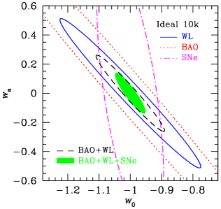
Figure 3.— Forecasts of 1$\sigma$ errors on the dark energy EOS parameters $w_{0}$ and $w_{\rm a}$ for the ideal 10k survey WL (solid line), BAOs (dotted line), SNe (dashed line), and the three combined (shaded area). We have included Planck priors in all the results. Although the CMB priors have a significant impact on the SN results and to a lesser degree on WL results and BAO results, they have a much smaller effect on the joint constraints of BAO+WL and BAO+WL+SNe.

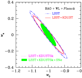
Figure 4.— Forecasts of 1$\sigma$ errors on the dark energy EOS parameters $w_{0}$ and $w_{\rm a}$ for LSST using BAO+WL (dash-dotted line), the combination of LSST and KDUST using BAO+WL (solid line, see Table 1), the combination of LSST and half of KDUST (labeled as KDUST5k) using BAO+WL (dotted line), and the combination of LSST and KDUST5k using BAO+WL+SNe (shaded area).

In summary, the parameter set includes 11 cosmological parameters and 170 nuisance parameters. The cosmological parameters are $w_{0}$, $w_{\rm a}$, the matter density $\omega_{\rm m}$, the baryon density $\omega_{\rm b}$, the angular size of the sound horizon at the last scattering surface $\theta_{\rm s}$, the curvature parameter $\Omega_{\rm k}$, the scalar spectral index $n_{\rm s}$, the running of the spectral index $\alpha_{\rm s}$, the primordial Helium fraction $Y_{\rm p}$, the election optical depth $\tau$, and the normalization of the primordial curvature power spectrum $\Delta_{\rm R}^{2}$. Note that $Y_{\rm p}$ and $\tau$ are solely constrained by the cosmic microwave background (CMB), which is introduced as priors. The nuisance parameters include 40 photo-z bias parameters, 40 photo-z rms parameters, 40 galaxy clustering bias parameters, 30 galaxy additive noise parameters, 10 shear additive noise parameters, and 10 parameters for shear calibration errors. We use multipoles $40\leq\ell\leq 2000$ for WL and $40\leq\ell\leq 3000$ for BAO. In addition, we require $\Delta_{\delta}^{2}(\ell/D_{A};z)<0.4$ for BAO to reduce the influence of nonlinear evolution. The lower cut in $\ell$ is to minimize the dependence of the forecasts on particular models of dark energy perturbation and the integrated Sachs–Wolfe effect, which affect only very large scales.

Figure 3 presents the forecasts of 1$\sigma$ error contours of the dark energy EOS parameters $w_{0}$ and $w_{\rm a}$ for the ideal 10k survey WL (solid line), BAO (dotted line), SNe (dot-dashed line), joint BAO and WL (dashed line), and the three combined (shaded area). Since different probes have different parameter degeneracy directions in the full parameter space, including both cosmological parameters and nuisance parameters (such as the photo-z bias and rms parameters), a joint analysis can reduce the error significantly. One example is that the BAO technique can determine the curvature parameter and the matter density far better than the SNe technique, whereas the latter needs strong priors on $\Omega_{\rm K}$ and $\omega_{\rm m}$ in order to place tight constraints on $w_{0}$ and $w_{\rm a}$ (Linder 2005; Knox et al. 2006b). Another example is that the WL technique is sensitive to the priors on the photo-z parameters, which can be calibrated by the BAO technique. By comparing the results in Figure 3 with the LSST BAO+WL result in Figure 4, one sees that the ideal 10,000 deg² ugrizyJH survey can place comparable constraints on the dark energy EOS parameters to the LSST survey.

We show the dark energy constraints from combinations of LSST with the KDUST 10,000 deg² survey and LSST with half of the KDUST survey (labeled as KDUST5k) in Figure 4. The KDUST5k survey could be carried out by a 2.5m KDUST pathfinder in 12 years. We assume that 5000 deg² high-resolution yJH imaging is enough to reach the systematic calibration floor, so the improvement to the LSST survey outside the KDUST survey area is kept the same for both proposals. Under this condition, the WL+BAO constraints on $w_{0}$ and $w_{a}$ from LSST+KDUST5k are nearly the same as those from LSST+KDUST; they improve the LSST-alone dark energy task force (DETF, Albrecht et al. 2006) figure of merit (FOM) by 30%. Adding SNAP-like SN data from KDUST as well can significantly increase the DETF FOM; the result is as good as LSST or LSST+KDUST joint BAO and WL constraints on $w_{0}$ and $w_{a}$ in the absence of systematics.

The current constraint on $\{w_{0},~{}w_{a}\}$ is (Zhao & Zhang 2010),

$$w_{0}=-0.90^{+0.11+0.23}_{-0.11-0.22},~{}w_{a}=-0.24^{+0.56+0.98}_{-0.55-1.2}.$$ (4)

derived from a joint Markov Chain Monte Carlo (MCMC) analysis of the recently released SNe “Constitution” sample (Hicken et al 2009), the WMAP five-year data (Komatsu et al 2009) , and the Sloan Digital Sky Survey (SDSS) Luminous Red Galaxy (LRG) sample (Tegmark et al 2006). In this analysis, the dark energy perturbation (DEP), which is important in the parameter estimation (Zhao et al. 2005; Fang, Hu & Lewis 2008), was consistently included based on the treatment developed in (Zhao et al. 2005). The central values indicate that the ‘quintom’ scenario (Feng, Wang & Zhang 2005) is mildly favored, namely, the EOS today $w(z)|_{z=0}=w_{0}>-1$, while EOS in the far past $w(z)|_{z=\infty}=w_{0}+w_{a}<-1$. This is consistent with the recent published result using the ‘Constitution’ SNe sample (Shafieloo, Sahni & Starobinsky 2009; Biswas & Wandelt 2009; Qi, Lu & Wang 2009; Wei 2009; Huang et al. 2009). The error bars in Equation 4 can be used to estimate the FOM of current data, and we find that KDUST+LSST can improve the current FOM by two orders of magnitude.

3.3. Principal Component Analysis on $w(z)$

To investigate the constraints on dark energy equation-of-state $w(z)$ from the surveys in a model-independent way, we follow (Huterer & Starkman 2002; Crittenden, Pogosian & Zhao 2009) and employ a Principle Component Analysis (PCA) approach.

We choose 40 uniform redshift bins, stretching to a maximum redshift of $z=3$, and allow the high redshift ($z>3$) equation of state to vary. To avoid $w(z)$ with infinite derivatives, each bin rises and falls following a hyperbolic tangent function with a typical transition width $dz$ of order 10% of the width of a bin. We choose a constant $w=-1.0$ as the fiducial model, which is consistent with all the present data. Since dark energy perturbations play a crucial role in the parameter estimation, we use a modified version of CAMB which allows us to calculate DEP for an arbitrary $w(z)$ consistently (Zhao et al. 2005).

For the PCA, we calculate the Fisher matrices based on four kinds of observables: supernovae, CMB anisotropies, galaxy number counts (GC) correlation functions and WL observations. We also include all the possible cross-correlations among these, including CMB$\times$galaxy and CMB$\times$WL, which are sensitive to the integrated Sachs-Wolfe effect, as well as galaxy-weak lensing correlations.

We first calculate the Fisher matrices for each of the observables, $F^{a}_{ij}$, where the indices $i,j$ run over the parameters of the theory, in our case the binned $w_{i}(z)$. We then find the normalized eigenvectors and eigenvalues of this matrix $\{e_{i}(z),\lambda_{i}\}$, and write

$$F=W^{T}\Lambda W,$$ (5)

where the rows of $W$ are the eigenvectors and $\Lambda$ is a diagonal matrix with elements $\lambda_{i}$. The Fisher matrix is an estimate of the inverse covariance matrix we expect the data to give us and the eigenvalues reflect how well the amplitude of each eigenvector can be measured. The true behavior of the equation of state can be expanded in the eigenvectors as

$$w(z)=w_{\rm fid}(z)+\sum_{i=1}^{N}\alpha_{i}e_{i}(z)$$ (6)

and the expected error in the recovered amplitudes is given by $\sigma(\alpha_{i})=\lambda_{i}^{-1/2}$.

For our forecasts, we assume three surveys: the ideal 10k survey, LSST and KDUST+LSST as listed in Table 1. We also combine the Planck survey for CMB and SNAP SNe. We assume a flat universe and marginalize over the intrinsic SN magnitude $M$ and the galaxy bias parameters.

In the upper panel of Figure 5, we show the spectra of eigenvalues $\sigma^{-2}(\alpha_{i})$ of the Fisher matrices for these three tomographic surveys, and in the lower panel, we show the ratio of the eigenvalues for LSST+KDUST to that for LSST. As we can see, the ideal 10k survey is competitive to LSST on the dark energy constraints, and adding KDUST to LSST can improve the constraints on the first few eigenmodes by as much as 85%. The first five best determined eigenvectors are shown in Figure 6. As we can see, the $N$th eigenmode has $N-1$ nodes in $z$, and the ‘sweet spot’ – the redshift where the uncertainty of $w(z)$ gets minimized – is at $z\sim 0.2$. This is consistent with the analysis done in (Huterer & Starkman 2002; Crittenden, Pogosian & Zhao 2009). We also find that adding KDUST to LSST makes the eigenmodes stretch to slightly higher $z$ because of the higher redshift reach with the addition of KDUST data.

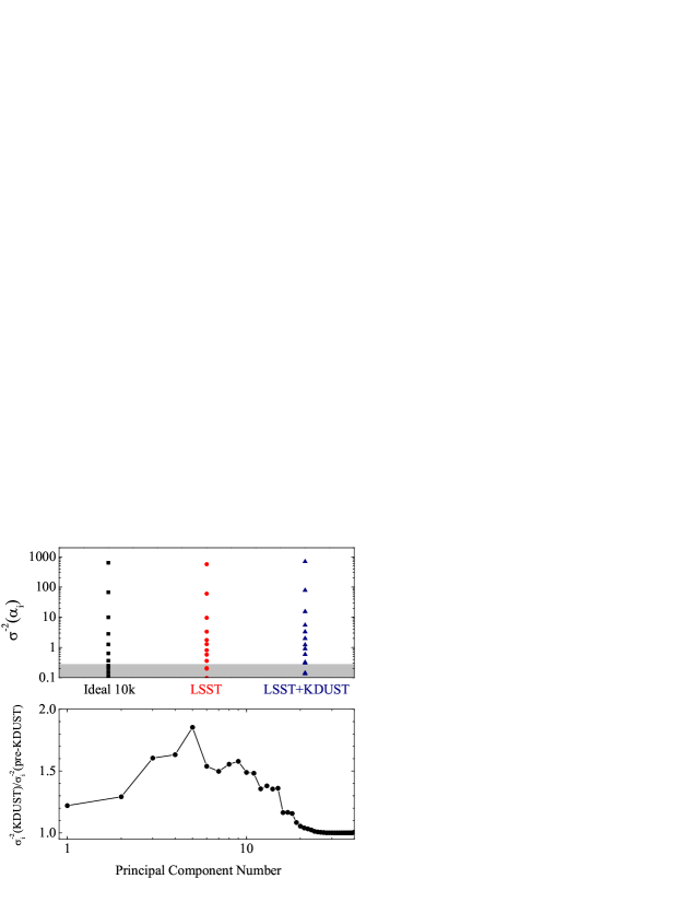
Figure 5.— Upper panel: The eigenvalues ($\sigma^{-2}(\alpha_{i})$) for the raw Fisher matrices (no priors assumed) for ideal 10k survey, LSST, and LSST+KDUST. The grey shaded region shows the diagonal prior of $\sigma_{\rm m}\geq 0.3$; Lower panel: The ratio of the eigenvalues ($\sigma^{-2}(\alpha_{i})$) for LSST+KDUST to that for LSST.

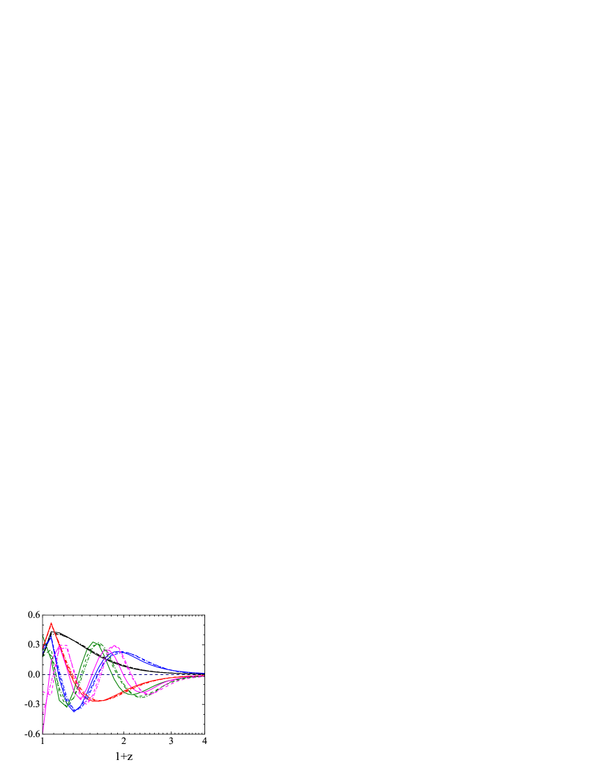
Figure 6.— The first five best determined eigenvectors for the ideal 10k survey (dashed lines), LSST (solid lines), and LSST+KDUST (dash-dotted lines). No priors have been assumed and the amplitudes are normalized to unity.

As stated in (Crittenden, Pogosian & Zhao 2009), all of the eigenvectors are informative, no matter how large the error bars are, if we have no prior knowledge of the possible $w(z)$ behaviors. However, even without a physical model for $w(z)$, we would still be surprised if $w(z)$ were much too positive ($w\gg 1/3$) or much too negative ($w\ll-1$). This motivates us to choose some theoretical priors to roughly separate the eigenmodes into those which are informative relative to the priors and those that are not. To apply the theoretical prior, we follow (Crittenden, Pogosian & Zhao 2009) to choose a correlation function describing fluctuations of $w(z)$ away from the fiducial model. This smoothness prior can filter out the high frequency modes, while the low frequency modes remain unaffected. Also, as long as there are sufficient bins compared to the correlation length, the prior largely wipes out dependence on the precise choice of binning.

As elaborated in (Crittenden, Pogosian & Zhao 2009), the deviations of the equation of state from its fiducial model can be encapsulated in a correlation function:

$$\xi_{w}(|z-z^{\prime}|)\equiv\left\langle(w(z)-w_{\rm fid}(z))(w(z^{\prime})-w_{\rm fid}(z^{\prime}))\right\rangle.$$ (7)

and the covariance matrix of the binned equation of state is then

$$\langle\delta w_{i}\delta w_{j}\rangle=\frac{1}{\Delta^{2}}\int_{z_{i}}^{z_{i}+\Delta}dz\int_{z_{j}}^{z_{j}+\Delta}dz^{\prime}\,\xi_{w}(|z-z^{\prime}|).$$ (8)

where the i^th bin is from $z_{i}$ to $z_{i}+\Delta$, and we assume that all bins have the same width $\Delta=z_{i+1}-z_{i}$. The variance of the mean equation of state over all the bins is,

$$\sigma_{\rm m}^{2}=\int_{0}^{z_{\rm max}}{dz}\int_{0}^{z_{\rm max}}{dz^{\prime}\over z_{\rm max}^{2}}\xi_{w}(z-z^{\prime}).$$ (9)

And we assume that $\xi_{w}(z)=\xi_{w}(0)/(1+(z/z_{c})^{2}).$ where $\xi_{w}(0)$ is the variance of $w$ at any given point and $z_{c}$ is the correlation length.

To apply the prior, we need to specify the correlation length $z_{c}$ and tune $\xi_{w}(0)$ so that the error in the mean, $\sigma_{\rm m}$ is in the range of $[0.2,0.5]$ in order to be consistent with the observational uncertainty. We tried correlation lengths in the range $0.1\leq z_{c}\leq 0.4$, where the upper limit was beginning to be strong enough to impact the observed modes for the SN. Then the resulting prior takes the form,

$${\cal{P}}_{\rm prior}\propto\exp{\left[-\frac{1}{2}({w}_{i}^{\rm true}-{w}_{i}^{\rm fid})C_{ij}^{-1}({w}_{j}^{\rm true}-{w}_{j}^{\rm fid})\right]}$$ (10)

where $C_{ij}\equiv\langle\delta w_{i}\delta w_{j}\rangle$. This prior naturally constrains the high frequency modes without over constraining the lower frequency modes that are typically probed by experiments.

Note that assuming no correlations among the bins is equivalent to using a delta function for the correlation prior, e.g. $\xi(z)=\xi_{0}\delta(z).$ In such a case, one finds $\langle\delta w_{i}\delta w_{j}\rangle=\xi_{0}\delta_{ij}/\Delta$ and the mean variance is $\sigma_{\rm m}^{2}=\xi_{0}/z_{\rm max}$. Thus, assuming a fixed total range, the bin variance should grow with the number of bins $\langle\delta w_{i}^{2}\rangle=\sigma_{\rm m}^{2}N_{\rm bins}$ to keep the mean variance unchanged.

In order to evaluate the value added by a given survey, we use the mean squared error (MSE) as a FOM. In the absence of any priors, this is expected to be

$${\rm MSE}={\rm Tr}\,F^{-1}.$$ (11)

Taking into account priors, $F$ in this expression is replaced by $C^{-1}+F$. The MSE arising from the prior alone is ${\rm MSE}={\rm Tr}~{}C$, and it is independent of the shape of the correlation function. Adding more experimental data reduces the MSE, and the amount by which the MSE is reduced can be seen as a measure of how informative the experiment is.

In Table 2, we vary $\xi_{w}(0)$ and $z_{c}$ while holding the prior constraint on the mean fixed, $\sigma_{\rm m}=0.3$. For the case of a diagonal prior, the MSE for the prior alone is given by $N_{\rm bins}\times\langle\delta w^{2}\rangle=N_{\rm bins}^{2}\sigma^{2}_{\rm m}=144.$ Adding the data, one could significantly improve the constraints on some of the eigenmodes, thus reduce the MSE. As the prior is diagonal, the new eigenmodes are also eigenmodes of the prior with the same eigenvalue, given by $N_{\rm bins}\sigma^{2}_{\rm m}=3.6$ (shaded region in the upper panels of Figure 5). The reduction of the MSE thus roughly tells us how many modes can be constrained compared to the prior. For example, adding LSST reduces the MSE from 144 to 112, meaning that there are $(144-112)/3.6\simeq 9$ modes can be constrained by LSST, and similarly, the ideal 10k survey is able to constrain 7 modes. With KDUST+LSST, one can actually constrain 10 eigenmodes. These numbers can also be counted in the upper panel of Figure 5 above the prior threshold shown in shade.

For a correlated prior, we can analogously put a lower bound on the number of modes constrained by data using the MSE shown in Table 2. For instance, for the case of $z_{c}=0.1$ and $z_{c}=0.4$, LSST combined with KDUST can at least constrain $(35-18.1)/3.6\simeq 4$ and $(11.5-3.7)/3.6\simeq 2$ modes, respectively. As we see, the number of new modes estimated in this way is reduced as the prior correlation length is increased. This is as expected – as $z_{c}$ increases, more high frequency modes will be filtered out by the smoothness prior.

Table 2The mean squared error for various priors and experiments.

	diagonal	$\,\,z_{c}=0.1\,\,$	$\,\,z_{c}=0.4$
no data	144.0	35.0	11.5
Ideal 10k	116.0 [7]	21.2	4.7
LSST	112.0 [9]	19.9	4.5
KDUST+LSST	108.3 [10]	18.1	3.7

4. Conclusion

Dome A offers a very competitive site for studying dark energy. Given the amount of resources required to build a large telescope and run a massive survey there, one must give the highest priority to programs that cannot be easily carried out elsewhere. Thus, a reasonable strategy is to focus on NIR imaging and collaborate with other surveys for optical data. Using LSST as an example, we show that a high-resolution 5000–10,000 deg² KDUST survey in yJH bands could improve LSST BAO+WL constraints on the dark energy EOS parameters $w_{0}$ and $w_{a}$ by reducing the photo-z and shear measurement systematics. A SNAP-like SN sample plus a large local and nearby SN sample from KDUST would further boost the DETF FOM by more than a factor of two.

In addition to forecasts for the $w_{0}$–$w_{a}$ parametrization, we also apply a PCA approach to investigate the constraints on the dark energy EOS $w(z)$ in a model-independent way. We find that regarding the number of the constrained eigenmodes of $w(z)$, an ideal 10,000 deg² ugrizyJH survey, combined with Planck, can constrain 7 eigenmodes, while KDUST+LSST can allow us to constrain 3 more modes.

We have not discussed dark energy probes such as strong lensing, cluster counting, and higher-order statistics of the same galaxy and shear data, which could further tighten the constraints on the dark energy EOS. Strong lensing constrains dark energy through the time delay effect as well as counting of strong lenses. It is also an excellent probe of dark matter halo structures and, hence, can be used to measure dark matter particle properties. With high-resolution imaging, one could extract more cosmological information from strong lensing observations. Therefore, Dome A could be particularly advantageous for strong lensing studies.

Dark energy forecasts depend crucially on the assumed properties of the survey data, including all the systematics. Dome A has many advantages over other ground sites and has an environment close to that in space. Hence, we use well-studied LSST and SNAP as references to make crude estimates of the data for this investigation. Further work and detailed modeling are needed to give a more realistic assessment of the Dome A site for studying dark energy.

References

- Abdalla et al. (2008) Abdalla, F.B., Amara, A., Capak, P., Cypriano, E.S., Lahav, O., & Rhodes, J. 2008, MNRAS, 387, 969
- Albrecht et al. (2006) Albrecht, A. et al.., ArXiv Astrophysics e-prints (2006), astro-ph/0609591.
- Ashley et al. (2010) Ashley et al., EAS Publications Series, Volume 40, 2010, pp.79-84
- Biswas & Wandelt (2009) Biswas, R. & Wandelt, B. D., arXiv:0903.2532 [astro-ph.CO].
- Blake & Glazebrook (2003) Blake, C., & Glazebrook, K. 2003, ApJ, 594, 665
- Bond & Efstathiou (1984) Bond J. R., & Efstathiou G., ApJ285, L45–L48 (1984).
- Chevallier & Polarski (2001) Chevallier M., & Polarski D., Int. J. Mod. Phys. D 10, 213 (2001).
- Cooray et al. (2001) Cooray, A., Hu, W., Huterer, D., & Joffre, M. 2001, ApJ, 557, L7
- Crittenden, Pogosian & Zhao (2009) Crittenden R. G., Pogosian L., & Zhao G. B., JCAP 0912,025 (2009).
- Dvali et al. (2000) Dvali G., Gabadadze G., & Porrati M., Phys. Lett. B 485, 208–214 (2000).
- Eisenstein et al. (1998) Eisenstein D. J., Hu W., & Tegmark M., ApJ504, L57 (1998).
- Fang, Hu & Lewis (2008) Fang W., Hu W., & Lewis A., Phys. Rev. D 78, 087303 (2008).
- Feng, Wang & Zhang (2005) Feng B., Wang X. L., & Zhang X. M., Phys. Lett. B 607, 35 (2005).
- Fossat et al. (2010) Fossat E. et al., arXiv:1003.3583 [astro-ph.IM]
- Hicken et al (2009) Hicken M.,et al., Astrophys. J. 700, 1097 (2009).
- Hu & Tegmark (1999) Hu, W., & Tegmark, M. 1999, ApJ, 514, L65
- Hu & Haiman (2003) Hu, W., & Haiman, Z. 2003, Phys. Rev. D, 68, 063004
- Hu & Jain (2004) Hu W., & Jain B., Phys. Rev. D70, 043009 (2004).
- Huang et al. (2009) Huang Q. G., Li M., Li X. D., & Wang S., Phys. Rev. D 80, 083515 (2009).
- Huterer (2002) Huterer, D. 2002, Phys. Rev. D, 65, 063001
- Huterer & Starkman (2002) Huterer D., & Starkman G., Phys. Rev. Lett. 90, 031301 (2003).
- Huterer et al. (2006) Huterer D., Takada M., Bernstein G., & Jain B., MNRAS366, 101–114 (2006).
- Jain et al. (2006) Jain, B., Jarvis, M., & Bernstein, G. 2006, Journal of Cosmology and Astro-Particle Physics, 2, 1
- Komatsu et al (2009) Komatsu E. et al. [WMAP Collaboration], Astrophys. J. Suppl. 180, 330 (2009).
- Kasliwal et al. (2008) Kasliwal, M. M., Massey, R., Ellis, R. S., Miyazaki, S., & Rhodes, J. 2008, ApJ, 684, 34
- Kim et al. (2010) Kim, A. et al. 2010, Astroparticle Physics, 33, 248
- Knox et al. (2005) Knox, L., Albrecht, A., & Song, Y.-S. 2005, in ASP Conf. Ser. 339: Observing Dark Energy, 107–+
- Knox et al. (2006a) Knox L., Song Y.-S., & Tyson J. A., Phys. Rev. D74, 023512 (2006a).
- Knox et al. (2006b) Knox L., Song Y.-S., & Zhan H., ApJ652, 857–863 (2006b), astro-ph/0605536.
- Linder (2003) Linder, E. V. 2003, Phys. Rev. D, 68, 083504
- Linder (2005) Linder E. V., Astroparticle Physics 24, 391–399 (2005).
- Linder (2004) Linder E. V., Phys. Rev. D70, 023511 (2004).
- LSST Science Collaborations (2009) LSST Science Collaborations: Paul A. Abell et al. 2009, ArXiv e-prints, 0912.0201
- Ma et al. (2006) Ma, Z., Hu, W., & Huterer, D. 2006, ApJ, 636, 21
- Massey et al. (2007) Massey, R. et al. 2007, MNRAS, 376, 13
- Paulin-Henriksson et al. (2008) Paulin-Henriksson, S., Amara, A., Voigt, L., Refregier, A., & Bridle, S. L. 2008, A&A, 484, 67
- Peebles & Yu (1970) Peebles P. J. E., & Yu J. T., ApJ162, 815 (1970).
- Perlmutter et al. (1999) Perlmutter S., et al., ApJ517, 565–586 (1999).
- Phillips (1993) Phillips M. M., ApJ413, L105–L108 (1993).
- Pogosian et al. (2005) Pogosian, L., Corasaniti, P. S., Stephan-Otto, C., Crittenden R., & Nichol R.,, Phys. Rev. D 72, 103519 (2005)
- Qi, Lu & Wang (2009) Qi S., Lu T., & Wang F. Y., arXiv:0904.2832 [astro-ph.CO].
- Refregier (2003) Refregier, A. 2003, ARA&A, 41, 645
- Riess et al. (1998) Riess A. G. et al., AJ116, 1009–1038 (1998).
- Saunders et al. (2009) Saunders, W. et al. 2009, PASP, 121, 976
- Schneider et al. (2006) Schneider, M., Knox, L., Zhan, H., & Connolly, A. 2006, ApJ, 651, 14
- Seo & Eisenstein (2003) Seo H., & Eisenstein D. J., ApJ598, 720–740 (2003).
- Shafieloo, Sahni & Starobinsky (2009) Shafieloo A., Sahni V., & Starobinsky A. A., arXiv:0903.5141 [astro-ph.CO].
- Spergel et al. (2007) Spergel D. N. et al., ApJS170, 377–408 (2007), arXiv:astro-ph/0603449.
- Takada & Jain (2004) Takada M., & Jain B., MNRAS348, 897–915 (2004).
- Tegmark (1997) Tegmark M., Phys. Rev. Lett. 79, 3806–3809 (1997).
- Tegmark et al (2006) Tegmark M. et al., Phys. Rev. D 74 123507 (2006).
- Tegmark et al. (2002) Tegmark, M. et al. 2002, ApJ, 571, 191
- Wei (2009) Wei H., arXiv:0906.0828 [astro-ph.CO].
- Wittman (2005) Wittman, D. 2005, ApJ, 632, L5
- Yang et al. (2009) Yang et al., Publications of the Astronomical Society of the Pacific, Volume 121, issue 876, pp.174-184
- Zhan (2006) Zhan H., JCAP, 8, 8 (2006), astro-ph/0605696.
- Zhan et al. (2009) Zhan, H., Knox, L., & Tyson, J. A. 2009, ApJ, 690, 923
- Zhang et al. (2009) Zhang, P., Pen, U., & Bernstein, G. 2009, ArXiv e-prints, 0910.4181
- Zhao, Huterer & Zhang (2007) Zhao G. B., Huterer D., & Zhang X., Phys. Rev. D 77, 121302 (2008).
- Zhao et al. (2009) Zhao G. B., Pogosian L., Silvestri A., & Zylberberg J., Phys. Rev. D 79, 083513 (2009)
- Zhao et al. (2005) Zhao G. B., Xia J. Q., Li M., Feng B. & Zhang X., Phys. Rev. D 72, 123515 (2005).
- Zhao & Zhang (2010) Zhao G. B., & Zhang X., Phys. Rev. D 81, 043518 (2010).
- Zou et al. (2010) Zou, H. et al. 2010, arXiv:1001.4951