Weighing the Universe with Photometric Redshift Surveys and the Impact on Dark Energy Forecasts

Abstract

With a wariness of Occam’s razor awakened by the discovery of cosmic acceleration, we abandon the usual assumption of zero mean curvature and ask how well it can be determined by planned surveys. We also explore the impact of uncertain mean curvature on forecasts for the performance of planned dark energy probes. We find that weak lensing and photometric baryon acoustic oscillation data, in combination with CMB data, can determine the mean curvature well enough that the residual uncertainty does not degrade constraints on dark energy. We also find that determinations of curvature are highly tolerant of photometric redshift errors.

1. Introduction

Due to indications from the CMB that the mean spatial curvature is close to zero, and the empirical successes of inflation, it has become quite common to assume that the mean curvature is exactly zero in analyses of current data (e.g. Spergel et al., 2003)) and in forecasting cosmological constraints to come from future surveys (e.g. Song & Knox, 2004)). Recently, however there has been renewed interest in the possibility of non-zero mean spatial curvature. For example, Linder (2005) explored the impact of dropping the flatness assumption on the ability of supernova + CMB data to determine dark energy parameters. Knox (2006) quantified how the combination of distance measurements into the dark energy dominated era, combined with CMB observations, could be used to determine the mean spatial curvature. Bernstein (2005) considered purely geometrical constraints on curvature to come from weak lensing (WL) and baryon acoustic oscillation (BAO) data. In this paper we extend Linder’s work to other cosmological probes (WL and BAO) and extend that of Knox (2006) by forecasting constraints on curvature to come from specific surveys rather than idealized measurements to single distances.

This renewed interest in mean curvature is due to several factors. First, the discovery of cosmic acceleration has made us wary of Occam’s razor, the idea that the simplest possible outcome is the most likely. Occam’s razor, before data convinced us otherwise, pointed toward a flat Universe with zero cosmological constant. Although zero mean spatial curvature is still consistent with the data, small departures are also still allowed. Given how Occam’s razor has misled us in the past, we trust the argument for simplicity less and lend more credence to the possibility of small, but non-zero, mean spatial curvature.

Second, recent theoretical work suggests that detectable amounts of mean spatial curvature from inflation may not be entirely improbable. Freivogel et al. (2006) estimate the probability distribution of $\Omega_{\rm tot}$ that follows from specific assumptions about the distribution of the shapes of potentials in the string-theory landscape. Taking $N=62$ as a lower bound on the number of e-foldings (in order to get $\Omega_{tot}>0.98$, their interpretation of the current lower bound) they find 10% of the probability in the range $62<N<64$ or roughly $0.02>1-\Omega_{\rm tot}>4\times 10^{-4}$. At face value this says that if we achieve the sensitivity to mean curvature possible with Planck and high-precision BAO measurements, as forecasted in Knox (2006), there will be a  10% chance of making a detection. Note, however, that possible volume factors in the measure, that could strongly favor Universes undergoing longer periods of inflation, were (knowingly) neglected. The importance of these measures is a controversial topic (e.g. Linde & Mezhlumian, 1995; Garriga et al., 1999).

Related to these two reasons is a third deriving from the importance for fundamental physics of a discovery that the dark energy is not a cosmological constant. The implications of such a discovery would be sufficiently dramatic that all the assumptions underlying it would need to be revisited. We risk making the following type of error: claiming detection of non-cosmological constant dark energy, when the data are actually explained by a cosmological constant plus curvature. Evidence for non-cosmological constant dark energy would stimulate the revisiting of many assumptions of the standard cosmological model, such as the adiabaticity of the primordial fluctuations (Trotta, 2003; Trotta & Durrer, 2004).

We are not declaring that dark energy conclusions reached by assuming $\Omega_{\rm K}=0$ are uninteresting. A result that informed us we need either non-$\Lambda$ dark energy or non-zero mean curvature would be frustratingly ambiguous, but nonetheless terribly interesting.

Here we quantify how well planned surveys can measure the mean spatial curvature as well as the impact of dropping the flatness assumption on the expected dark energy constraints. In section  2 we describe our modeling of the surveys considered, including systematic errors from, e.g., supernova mean absolute magnitude evolution and photometric redshift errors. In section  3 we show the constraints on mean curvature from these surveys individually and in combinations. In section  4 we do the same for dark energy. Finally, in Section  5 we discuss and conclude.

As an historical aside we note that our title alludes to an earlier paper “Weighing the Universe with the CMB” (Jungman et al., 1996) that pointed out the sensitivity of the location of the CMB acoustic peak to the mean curvature, and thus the mean density (in units of the critical density). Since then CMB observations have indeed been used to greatly improve the precision with which the mean curvature is known (Miller et al., 1999; Dodelson & Knox, 2000; de Bernardis et al., 2000) and most recently Spergel et al. (2006). Further improvements in precision require determinations of distances to redshifts much lower than that of the last-scattering surface (Eisenstein et al., 2005; Knox, 2006) made possible by the surveys we discuss here.

2. Surveys

The three probes we consider here are probes of the dark energy via the distance-redshift relation, $D(z)$. Weak lensing is also sensitive to dark energy via its influence on the growth of large-scale structure. We first emphasize their qualitative distinguishing characteristics before moving on to a description of the specific surveys we consider and how we model them.

Supernovae (SN) determine the shape of the distance-redshift curve, but not an overall amplitude. Planned space-based supernova surveys probe this relation out to $z\simeq 1.7$ (e.g. Aldering, 2005). Toward higher redshifts spectral features used to type the supernovae are at wavelengths to which the detectors are not sensitive. The detectors are transparent at these wavelengths by design, to reduce thermal noise. Although JWST will be capable of detecting supernovae at higher redshifts, one can expect greater evolutionary effects at these redshifts. Indeed, Riess & Livio (2006) recently pointed out that JWST could be used to study evolutionary effects at $z\simeq 2$ so that they can be better understood at lower redshifts. Also, gravitational lensing contributes to the luminosity dispersion and this contribution increases with redshift (Holz, 1998).

Baryon acoustic oscillations (BAO) also determine the shape of the $D(z)$ curve, by exploiting a standard ruler in the galaxy power spectrum. The length of this ruler, the sound horizon at the epoch of CMB last scattering, can be accurately determined from CMB observations, thus giving us the amplitude of the $D(z)$ relation as well. This technique can be used to redshifts of 3 and beyond.

Weak lensing (WL) observations constrain the $D(z)$ curve in a less direct manner. For forecasts of $D(z)$ and growth factor $g(z)$ reconstructions from WL data see Knox et al. (2005). For an excellent discussion of the origin of the $D(z)$ constraints from WL see Zhang et al. (2005). Like BAO, WL can be used to study $D(z)$ to redshifts of 3 and beyond. Unlike SN and BAO, the WL technique is sensitive to the growth of structure, which can also contribute significantly to the constraints on dark energy (Zhang et al., 2005).

The SN technique can achieve strong constraints on $D(z)$ with a sufficiently small number of sufficiently bright objects that a survey can be designed that allows for spectroscopic redshifts to be determined for all the objects. In contrast, weak lensing observations rely on the shape determinations of very large numbers of very faint galaxies, making spectroscopy prohibitively expensive. Instead, one must rely on photometrically-determined redshifts. The demands on control of systematic errors on these redshifts are quite stringent (Bernstein & Jain, 2004; Ma et al., 2006; Huterer & Cooray, 2005). If spectroscopy is used then the BAO technique requires fewer galaxies than are required by WL; interesting constraints are possible from ambitious, but achievable, spectroscopic surveys (e.g. Seo & Eisenstein, 2003). Here we only consider BAO surveys that forego spectroscopy and thus rely on photometric redshifts. We have previously argued that photometric BAO surveys also place stringent demands on the level of required systematic error control (Zhan & Knox, 2005). Although, if one gives up the radial information and uses tomographic galaxy angular power spectra, the demands can be greatly reduced (Zhan 2006, in preparation).

We allow the following cosmological parameters to vary in our forecasts: the dark energy equation-of-state parameters $w_{0}$ and $w_{a}$ as defined by $w(a)=w_{0}+w_{a}(1-a)$, the matter density $\omega_{\rm m}$, the baryon density $\omega_{\rm b}$, the angular size of the sound horizon at the last scattering surface $\theta_{\rm s}$, the equivalent matter fraction of curvature $\Omega_{\rm K}$, the optical depth to scattering by electrons in the reionized inter-galactic medium, $\tau$, the primordial helium mass fraction $Y_{\rm p}$, the spectral index $n_{\rm s}$ of the primordial scalar perturbation power spectrum, the running of the spectral index $\alpha$, and the normalization of the primordial curvature power spectrum $\Delta_{R}^{2}$ at $k=0.05\,\mbox{Mpc}^{-1}$. The fiducial model has $(w_{0},w_{a},\omega_{\rm m},\omega_{\rm b},\theta_{\rm s},\Omega_{\rm K},\tau,Y_{\rm p},n_{\rm s},\alpha,\Delta_{R}^{2})=(-1,0,0.127,0.0223,0.596\,\deg,0,0.09,0.24,0.951,0,2\times 10^{-9})$. This model is consistent with the 3-year WMAP data (Spergel et al., 2006) and has a reduced Hubble constant of $h=0.73$.

2.1. Supernovae

Our fiducial supernova data set has 3000 supernovae from a space-based survey distributed in redshift uniformly from $z=0.4$ to $z=1.7$, 700 supernovae from a ground-based survey distributed uniformly in redshift from $z=0.2$ to $z=0.7$ and 500 supernovae from a local sample distributed from $z=0.02$ to $z=0.1$. We model the supernova effective apparent magnitudes, after standardization (e.g., by exploitation of the Phillips relation (Phillips, 1993)), as

$$m_{i}=M+\alpha_{1}z_{i}+\alpha_{2}z_{i}^{2}+5\log_{10}(D_{L}(z_{i})/10{\rm pc})+n_{i}$$ (1)

where $M$ is the (unknown) absolute magnitude of a $z=0$ standardized supernova, the $z$ and $z^{2}$ terms allow for a drift in this mean due to evolution effects or other systematic errors and $n_{i}$ is from any random sources of scatter, either intrinsic to the supernovae or measurement noise.

We assume $\langle n_{i}n_{j}\rangle=\sigma^{2}\delta_{ij}$ with $\sigma=0.14$ and further that we are able to constrain the systematic error terms well enough to place Gaussian priors on their distributions with standard deviations $\sigma_{P}(\alpha_{1})=\sigma_{P}(\alpha_{2})=0.015$.

2.2. Weak Lensing

Our fiducial WL survey is modeled after LSST. We use the source-redshift distribution $n(z)=n_{0}z^{2}e^{-z/0.5}$ with $n_{0}$ chosen so the total source density is 50 galaxies per sq. arcmin. We assume the shape noise variance increases with redshift as $\gamma_{\rm rms}(z)=0.18+0.042z$. We take $40\leq\ell\leq 2000$ and a sky coverage of 20,000 square degrees.

We divide the galaxies into nine photometric redshift (photo-z) bins evenly spaced from $z_{\rm p}=0$ to $3.5$, where the subscript $p$ distinguishes photo-zs from true redshifts. Uncertainties in the error distribution of photo-zs are treated as in Ma et al. (2006). Specifically, we define an rms photo-z standard deviation $\sigma_{z}$ and a photo-z bias $\delta z$ at each of 35 redshift values evenly spaced over the range $z_{\rm p}=0$ to $3.5$. The photo-z bias and rms at an arbitrary redshift are linearly interpolated from the 70 parameters. This treatment of photo-z uncertainties is based on our expectation that photo-z calibrations through spectroscopy and other means (e.g. Schneider et al. 2006, in preparation; Newman 2006, in preparation) will be available, though challenging, at redshift intervals of width $\sim 0.1$.

We adopt a conservative estimate of the rms photo-z error of $\sigma_{z}=0.06(1+z)$ with $\delta z=0$. Smaller dispersions have been achieved for the CFHT Legacy Survey for a sample of galaxies with $i^{\prime}_{\rm AB}$ magnitudes less than 24 and $z\lesssim 2$(Ilbert et al., 2006) . We assume that through a calibration process we will know the photo-z bias parameters to within $\pm\sigma_{P}(\delta z_{i})$ which in the following ranges from an optimistic 0.001 to a pessimistic 0.01. The prior we assume for the rms parameter takes on a similar range. To reduce the dimensions of the parameter space we explore, we always set $\sigma_{P}(\sigma_{zi})=\sqrt{2}\sigma_{P}(\delta z_{i})$.

2.3. Baryon Acoustic Oscillations

Our BAO survey uses the same galaxies and photo-z parameters as the WL survey. We only include the angular power spectrum in our forecast, not the redshift-space power spectrum, because to extract information from the radial clustering one has to meet very stringent photo-z requirements (Zhan & Knox, 2005).

Unlike the WL shear power spectrum, the galaxy angular power spectrum has a narrow kernel, which is the radial galaxy distribution in the true-redshift space. Hence, one can use more photo-z bins for BAO until shot noise overwhelms the signal or the bin sizes are much smaller than the rms photo-z errors (Zhan, in preparation). For this work, we divide the galaxies into 30 photo-z bins from $z_{\rm p}=0.15$ to $3.5$ with bin size proportional to $1+z$.

To avoid contamination by nonlinearity, we exclude modes that have the dimensionless power spectrum $\Delta^{2}(k)>0.4$, e.g., $k_{\rm max}\sim 0.15\,h\,\mbox{Mpc}^{-1}$ or $\ell_{\rm max}=68$ at $z=0.15$. We then only use multipoles $40\leq\ell\leq 3000$ for BAO.

We treat the galaxy clustering bias in the same way as the photo-z parameters, i.e., we assign 35 bias parameters $b_{i}$ uniformly from $z=0$ to $3.5$ and linearly interpolate the values. The fiducial bias model is $b=1+0.84z$, and we apply a prior of 20% to each bias parameter.

We implement the method by Hu & Jain (2004) to combine BAO and WL. Note, however, that we do not use the halo model to calculate the galaxy bias, since we restrict our analysis to largely linear scales.

2.4. CMB and $H_{0}$

We calculate a Fisher matrix from the CMB data expected from Planck, following the treatment in (Kaplinghat et al., 2003). We also create a Fisher matrix for the HST Key Project Hubble constant determination (Freedman et al., 2001) by projecting a Hubble constant constraint of $\sigma_{\rm P}[\ln H_{0}]=0.11$ into our parameter space. We add both these Fisher matrices to all of the Fisher matrices calculated for the dark energy probes. Of course, when plotting combinations we are careful to only add these Fisher matrices in once to avoid double-counting the $H_{0}$ and CMB information.

2.5. Systematic Errors

The surveys we consider, if they are to achieve the errors we forecast below, will need to achieve exquisite control of systematic errors. Our data modeling includes photometric redshift errors and supernova evolution but not many other sources of systematic error. Even for these that we do include, our modeling may not be sufficiently general to adequately model the real world. We need more data to know for sure.

For further discussion of systematic errors from a space-based SN mission see Kim et al. (2004). For WL we have not included galaxy shape measurement systematics (see e.g. Huterer et al., 2006) and intrinsic alignments, most importantly alignments between source galaxies and shear (Hirata & Seljak, 2004; Mandelbaum et al., 2006). For further discussion of these effects, see the technical appendix of the impending report of the Dark Energy Task Force (DETF). Also note that recent work with archival Subaru data demonstrates that very low levels of spurious additive shear are achievable from the ground (Wittman, 2005). For BAO, perhaps the major concern is spatially varying photometric offsets. Controlling photometry offsets at the requisite levels was a significant challenge for the recent BAO analysis from SDSS photometric data (Padmanabhan et al., 2006). Spatially variable dust extinction must be controlled as well, as discussed in Zhan et al. (2006).

3. Curvature

Figure 1.— Redshift error priors vs. $\sigma(\Omega_{\rm K})$ for various data sets and combinations.

Results for curvature are shown in Fig. 1. The first striking feature is the robustness to the quality of the photometric redshifts. This behavior is in contrast to that of the dark energy constraints from weak lensing as calculated in Bernstein & Jain (2004); Ma et al. (2006); Huterer et al. (2006) and in the next section.

For the supernova curve this robustness is trivial; we assume a spectroscopic survey for the supernovae and hence the results, by design, are completely independent of the photometric redshift parameters. For WL and BAO the near lack of dependence has its origins in the critical role played by measurements of distances to redshifts in the matter-dominated era (Knox, 2006). The comoving angular-diameter distance varies very slowly with $z$ at $z\gtrsim 2$, and hence the tolerance to redshift errors is quite high.

The value of $\sigma(\Omega_{\rm K})$ achieved depends on which probe is used. Those that reach to larger redshifts (WL and BAO) are protected from the confusing effects of dark energy and thus do a better job of determining $\Omega_{\rm K}$. WL and BAO data sets, either individually or in combination, can be used to determine $\Omega_{\rm K}$ at about the $10^{-3}$ level, consistent with the much more model-independent estimates in Knox (2006).

In addition to the shorter redshift reach, another important difference of the SN probe is the lack of strong normalization of $D(z)$. This can be remedied by a better measurement of the Hubble constant. Improving the Hubble constant prior to 1% reduces the supernova $\sigma(\Omega_{\rm K})$ to 0.004.

These forecasts for curvature are correct if the dark energy is parameterized by $w_{0}$, $w_{a}$ and $w_{0}+1\simeq w_{a}\simeq 0$. If the dark energy density is more important at higher redshifts than in our fiducial model, then the constraints will weaken somewhat.

If the history of the dark energy equation-of-state parameter is not well-approximated by our assumed form, and has a density higher at $z\gtrsim 3$ than its current value, then we risk significant systematic errors in our determination of $\Omega_{\rm K}$. We can partially guard against this error by verifying that $w_{0}$ and $w_{a}$ can be adjusted to give a good fit to the data. The worry remains though that unexpectedly high dark energy density at $3<z<1100$ could mimic a small negative curvature.

How much model dependence will obscure our determination of the curvature depends on how the experimental program plays out. One of the most interesting possible results is that $K$ is determined to be greater than zero ($\Omega_{\rm K}<0$) with high confidence. Such a result would be difficult to reconcile with inflation because short inflation scenarios solve the horizon problem by bubble nucleation which leads to $K>0$. A determination that $K>0$ would be challenging to the whole string theory landscape paradigm. Further, it would be robust to the systematic error described above, since unexpectedly high dark energy density, if unaccounted for, would mean the true value of $K$ is even larger.

Bernstein (2005) pointed out that gravitational lensing’s sensitivity to the source-lens angular-diameter distance means that the curvature could be determined in a manner independent of assumptions about $H(z)$. Bernstein’s effect contributes to the curvature constraints we forecast, but at a highly subdominant level. Were we to allow more freedom in the possible time variations of the dark energy density Bernstein’s effect would become important. Its independence of Einstein’s equations is an interesting virtue.

4. Dark Energy

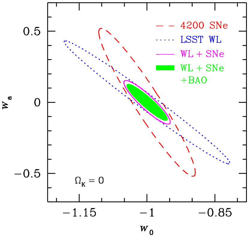
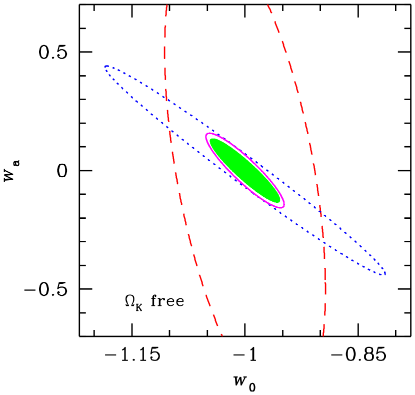
Figure 2.— Left panel: 1, 68% confidencce error contours of $w_{0}$ and $w_{a}$ assuming a flat universe. The contours are shown for 4200 SNe (dashed line), LSST WL (dotted line), the combination WL + SN (solid line), and the combination WL + SN + BAO (shaded area). All results include Planck and $H_{0}$ priors and assume $\sigma_{\rm P}(\delta z)=\sigma_{\rm P}(\sigma_{z})/\sqrt{2}=0.003$. Right panel: the same as the left panel but with $\Omega_{\rm K}$ treated as a free parameter.

The SN, WL, and BAO constraints on $w_{0}$ and $w_{a}$ are given in Figure 2 with (left panel) and without (right panel) assuming a flat universe. The SN constraint (dashed lines) on $w_{a}$ is very sensitive to curvature (as shown by Linder, 2005), whereas WL (dotted lines), being able to determine the curvature parameter $\Omega_{\rm K}$ to $\sim 0.001$ (see Figure 1), is not. Hence their combination (solid lines) is only slightly affected by adding $\Omega_{\rm K}$ as a free parameter.

The degeneracy between $\Omega_{\rm K}$ and $w(a)$ given SN data can be understood as follows. The SN data (with no CMB or $H_{0}$ data added) are only sensitive to $\Omega_{m}$, $\Omega_{\rm K}$ and $w(a)$. Including the constraint from the CMB on the distance to last scattering can be thought of as pinning down one combination of $\Omega_{m}$ and $\Omega_{K}$. The remaining degree of freedom has some degeneracy with $w(a)$ and is what is responsible for degrading the $w(a)$ constraints. Including an $\Omega_{m}$ prior would provide the one extra constraint necessary to remove the degeneracy. As Linder (2005) showed, the results with a prior $\sigma(\Omega_{m})=0.01$ are very similar to the results with curvature fixed. Similar improvements would come from a strong Hubble constant prior since, combined with Planck’s determination of $\Omega_{m}h^{2}$ to better than 1%, this can be translated into a determination of $\Omega_{m}$. The importance of $H_{0}$ for dark energy probes has been stressed by Hu (2005).

We now turn to the dependence of our forecasted dark energy constraints on photometric redshift errors. We show our results in Figure 3. Specifically, we plot $\sigma(w_{p})\times\sigma(w_{a})$ as we change the priors on the mean redshift of each redshift bin and the rms of the scatter in each redshift bin. Hu & Jain (2003) introduced the variable $w_{p}=w(a_{p})$ where $a_{p}$ is the scale factor at which $w(a)$ is determined with the smallest uncertainty, assuming that $w(a)=w_{0}+(1-a)w_{a}$. From this definition it also follows that the errors on $w_{p}$ and $w_{a}$ are uncorrelated with each other. The product $\sigma(w_{p})\times\sigma(w_{a})$ is proportional to the area of the $w_{0}$, $w_{a}$ 95% confidence ellipse. The inverse of this product is proportional to the figure of merit used by the DETF, recently discussed by Martin & Albrecht (2006) and Linder (2006).

Just as in Figure 1 the SN alone case is a horizontal line because the photo-z parameters have nothing to do with the SN data. We also see the dependence of $\sigma(w_{p})\times\sigma(w_{a})$ for WL on the photometric redshift parameters. For these forecasts we have marginalized over all of our other parameters, including curvature. With curvature fixed the SN alone case would improve from $\sigma(w_{p})\times\sigma(w_{a})=0.04$ to 0.004.

The BAO alone results are worse than WL alone. To understand why we also plot results for BAO in the limit of perfect prior knowledge of the bias parameters. In this limit the galaxy survey is also sensitive to growth so we label the dashed curve as BAO+g. This (unrealistic) case performs better than WL. This is as we expect since the galaxy power spectra give us finer spatial and temporal sampling of the dark matter power spectra than we get from weak lensing with its broad kernels. Likewise, we artificially remove all growth information from WL by pretending that the gravitational potentials are sourced by some unknown bias factors times the dark matter density, factors that we then marginalize over. We parameterize this b(z) in the same manner as we do with BAO. We see in the dot-dashed curve labeled WL-g that the WL results are worse than BAO if we are unable to predict the growth rate from our (non-bias) model parameters.

An interesting feature of the BAO result is its near-independence of photo-z parameters. Since the effect of photo-z uncertainties is more localized in redshift space for galaxy angular power spectra, BAO data allow for useful constraints on the photo-z parameters and therefore the dark energy constraints are less sensitive to photo-z priors (Zhan 2006, in preparation). By combining BAO and WL, one can achieve dark energy constraints that are robust to the dominant uncertainties of either probes: the galaxy bias for BAO and photo-z distribution for WL.

Note that the experiment-combining procedure used for the DETF report assumes that systematic error parameters for each experiment are independent. Taking the photo-z parameters to be the same for WL and BAO is an important difference and makes our BAO + WL combination significantly more powerful than in the DETF report. To take advantage of this synergy with real data, the analysis will either have to be done so that the galaxies used for their correlation properties and those used for their shape properties are weighted in the same manner, or the differences in the populations used for WL and BAO will have to be modeled.

SN can measure relative distances more accurately at low redshift than at high redshift. In contrast, the smaller volumes available at low redshift make WL and BAO distance and growth constraints weaker toward lower redshifts. This complementarity leads to remarkable reductions of the product $\sigma(w_{p})\times\sigma(w_{a})$ from combinations of SN with BAO or WL, as shown in Fig. 3. The complementarity is reflected in the orientations of the error ellipses of WL and SN in Fig. 2 as well. Furthermore, WL and/or BAO provide a normalization of the $D(z)$ curve, and a strong constraint on curvature as discussed in the previous section. Given the curvature constraints from WL/BAO, the SN $w_{0}$–$w_{a}$ error ellipse is nearly the same as that for a flat Universe. Hence, the combination SN+WL does not change appreciably with the curvature prior.

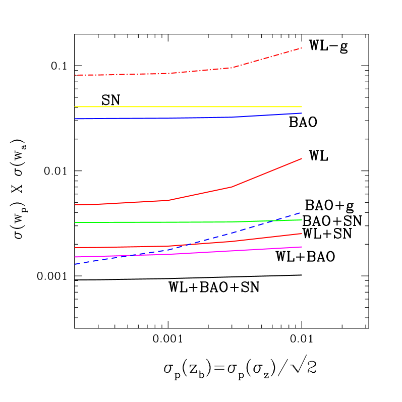
Figure 3.— Redshift error priors vs. the dark energy equation-of-state parameter error product $\sigma(w_{p})\times\sigma(w_{a})$ for various data sets and combinations. See text for explanations of BAO+g and WL-g.

5. Conclusions

Precision measurements of the mean curvature are interesting in their own right and also important for reaching conclusions about dark energy, due to the dark energy-curvature degeneracy. We found that the WL and BAO datasets, as we modeled them, would be capable of constraining $\Omega_{\rm K}$ at the $10^{-3}$ level. This tight constraint is highly robust to photometric redshift errors, much more so than is the case for the dark energy parameters, especially for WL. Further, the tight constraint essentially breaks the dark energy-curvature degeneracy.

There are many challenges that must be met so that real surveys can achieve our forecasted parameter constraints. We have addressed one which has been given much attention recently: photometric redshift errors. We find that, given our (70-parameter) photometric redshift error model, and conservative prior information on the parameters of this model, the galaxy correlations serve to control the parameters of the model well enough that the combined WL + BAO constraints on curvature and dark energy are very strong.

References

- Aldering (2005) Aldering, G. 2005, New Astronomy Review, 49, 46
- Bernstein (2005) Bernstein, G. 2005, ArXiv Astrophysics e-prints
- Bernstein & Jain (2004) Bernstein, G. & Jain, B. 2004, ApJ, 600, 17
- de Bernardis et al. (2000) de Bernardis, P., Ade, P. A. R., Bock, J. J., Bond, J. R., Borrill, J., Boscaleri, A., Coble, K., Crill, B. P., De Gasperis, G., Farese, P. C., Ferreira, P. G., Ganga, K., Giacometti, M., Hivon, E., Hristov, V. V., Iacoangeli, A., Jaffe, A. H., Lange, A. E., Martinis, L., Masi, S., Mason, P. V., Mauskopf, P. D., Melchiorri, A., Miglio, L., Montroy, T., Netterfield, C. B., Pascale, E., Piacentini, F., Pogosyan, D., Prunet, S., Rao, S., Romeo, G., Ruhl, J. E., Scaramuzzi, F., Sforna, D., & Vittorio, N. 2000, Nature, 404, 955
- Dodelson & Knox (2000) Dodelson, S. & Knox, L. 2000, Physical Review Letters, 84, 3523
- Eisenstein et al. (2005) Eisenstein, D. J., Zehavi, I., Hogg, D. W., Scoccimarro, R., Blanton, M. R., Nichol, R. C., Scranton, R., Seo, H.-J., Tegmark, M., Zheng, Z., Anderson, S. F., Annis, J., Bahcall, N., Brinkmann, J., Burles, S., Castander, F. J., Connolly, A., Csabai, I., Doi, M., Fukugita, M., Frieman, J. A., Glazebrook, K., Gunn, J. E., Hendry, J. S., Hennessy, G., Ivezić, Z., Kent, S., Knapp, G. R., Lin, H., Loh, Y.-S., Lupton, R. H., Margon, B., McKay, T. A., Meiksin, A., Munn, J. A., Pope, A., Richmond, M. W., Schlegel, D., Schneider, D. P., Shimasaku, K., Stoughton, C., Strauss, M. A., SubbaRao, M., Szalay, A. S., Szapudi, I., Tucker, D. L., Yanny, B., & York, D. G. 2005, ApJ, 633, 560
- Freedman et al. (2001) Freedman, W. L., Madore, B. F., Gibson, B. K., Ferrarese, L., Kelson, D. D., Sakai, S., Mould, J. R., Kennicutt, R. C., Ford, H. C., Graham, J. A., Huchra, J. P., Hughes, S. M. G., Illingworth, G. D., Macri, L. M., & Stetson, P. B. 2001, ApJ, 553, 47
- Freivogel et al. (2006) Freivogel, B., Kleban, M., Rodríguez Martínez, M., & Susskind, L. 2006, Journal of High Energy Physics, 3, 39
- Garriga et al. (1999) Garriga, J., Tanaka, T., & Vilenkin, A. 1999, Phys. Rev. D, 60, 023501
- Hirata & Seljak (2004) Hirata, C. M. & Seljak, U. 2004, Phys. Rev. D, 70, 063526
- Holz (1998) Holz, D. E. 1998, ApJ, 506, L1
- Hu (2005) Hu, W. 2005, in ASP Conf. Ser. 339: Observing Dark Energy, ed. S. C. Wolff & T. R. Lauer, 215–+
- Hu & Jain (2003) Hu, W. & Jain, B. 2003, ArXiv Astrophysics e-prints
- Hu & Jain (2004) —. 2004, Phys. Rev. D, 70, 043009
- Huterer & Cooray (2005) Huterer, D. & Cooray, A. 2005, Phys. Rev. D, 71, 023506
- Huterer et al. (2006) Huterer, D., Takada, M., Bernstein, G., & Jain, B. 2006, MNRAS, 366, 101
- Ilbert et al. (2006) Ilbert, O., Arnouts, S., McCracken, H. J., Bolzonella, M., Bertin, E., Le Fevre, O., Mellier, Y., Zamorani, G., Pello, R., Iovino, A., Tresse, L., Bottini, D., Garilli, B., Le Brun, V., Maccagni, D., Picat, J. P., Scaramella, R., Scodeggio, M., Vettolani, G., Zanichelli, A., Adami, C., Bardelli, S., Cappi, A., Charlot, S., Ciliegi, P., Contini, T., Cucciati, O., Foucaud, S., Franzetti, P., Gavignaud, I., Guzzo, L., Marano, B., Marinoni, C., Mazure, A., Meneux, B., Merighi, R., Paltani, S., Pollo, A., Pozzetti, L., Radovich, M., Zucca, E., Bondi, M., Bongiorno, A., Busarello, G., De La Torre, S., Gregorini, L., Lamareille, F., Mathez, G., Merluzzi, P., Ripepi, V., Rizzo, D., & Vergani, D. 2006, ArXiv Astrophysics e-prints
- Jungman et al. (1996) Jungman, G., Kamionkowski, M., Kosowsky, A., & Spergel, D. N. 1996, Physical Review Letters, 76, 1007
- Kaplinghat et al. (2003) Kaplinghat, M., Knox, L., & Song, Y. 2003, ArXiv Astrophysics e-prints, 3344
- Kim et al. (2004) Kim, A. G., Linder, E. V., Miquel, R., & Mostek, N. 2004, MNRAS, 347, 909
- Knox (2006) Knox, L. 2006, Phys. Rev. D, 73, 023503
- Knox et al. (2005) Knox, L., Song, Y. ., & Tyson, J. A. 2005, ArXiv Astrophysics e-prints
- Linde & Mezhlumian (1995) Linde, A. & Mezhlumian, A. 1995, Phys. Rev. D, 52, 6789
- Linder (2005) Linder, E. V. 2005, Astroparticle Physics, 24, 391
- Linder (2006) —. 2006, ArXiv Astrophysics e-prints
- Ma et al. (2006) Ma, Z., Hu, W., & Huterer, D. 2006, ApJ, 636, 21
- Mandelbaum et al. (2006) Mandelbaum, R., Hirata, C. M., Ishak, M., Seljak, U., & Brinkmann, J. 2006, MNRAS, 367, 611
- Martin & Albrecht (2006) Martin, D. & Albrecht, A. 2006, ArXiv Astrophysics e-prints
- Miller et al. (1999) Miller, A. D., Caldwell, R., Devlin, M. J., Dorwart, W. B., Herbig, T., Nolta, M. R., Page, L. A., Puchalla, J., Torbet, E., & Tran, H. T. 1999, ApJ, 524, L1
- Padmanabhan et al. (2006) Padmanabhan, N., Schlegel, D. J., Seljak, U., Makarov, A., Bahcall, N. A., Blanton, M. R., Brinkmann, J., Eisenstein, D. J., Finkbeiner, D. P., Gunn, J. E., Hogg, D. W., Ivezic, Z., Knapp, G. R., Loveday, J., Lupton, R. H., Nichol, R. C., Schneider, D. P., Strauss, M. A., Tegmark, M., & York, D. G. 2006, ArXiv Astrophysics e-prints
- Phillips (1993) Phillips, M. M. 1993, ApJ, 413, L105
- Riess & Livio (2006) Riess, A. G. & Livio, M. 2006, ArXiv Astrophysics e-prints
- Seo & Eisenstein (2003) Seo, H. & Eisenstein, D. J. 2003, ApJ, 598, 720
- Song & Knox (2004) Song, Y. & Knox, L. 2004, Phys. Rev. D, 70, 063510
- Spergel et al. (2006) Spergel, D. N., Bean, R., Dore’, O., Nolta, M. R., Bennett, C. L., Hinshaw, G., Jarosik, N., Komatsu, E., Page, L., Peiris, H. V., Verde, L., Barnes, C., Halpern, M., Hill, R. S., Kogut, A., Limon, M., Meyer, S. S., Odegard, N., Tucker, G. S., Weiland, J. L., Wollack, E., & Wright, E. L. 2006, ArXiv Astrophysics e-prints
- Spergel et al. (2003) Spergel, D. N., Verde, L., Peiris, H. V., Komatsu, E., Nolta, M. R., Bennett, C. L., Halpern, M., Hinshaw, G., Jarosik, N., Kogut, A., Limon, M., Meyer, S. S., Page, L., Tucker, G. S., Weiland, J. L., Wollack, E., & Wright, E. L. 2003, ApJS, 148, 175
- Trotta (2003) Trotta, R. 2003, New Astronomy Review, 47, 769
- Trotta & Durrer (2004) Trotta, R. & Durrer, R. 2004, ArXiv Astrophysics e-prints
- Wittman (2005) Wittman, D. 2005, ApJ, 632, L5
- Zhan & Knox (2005) Zhan, H. & Knox, L. 2005, ArXiv Astrophysics e-prints
- Zhan et al. (2006) Zhan, H., Knox, L., Tyson, J. A., & Margoniner, V. 2006, ApJ, 640, 8
- Zhang et al. (2005) Zhang, J., Hui, L., & Stebbins, A. 2005, ApJ, 635, 806