Perspectives of High Energy Neutrino Astronomy

Abstract

This work discusses the perspectives to observe fluxes of high energy astrophysical neutrinos with the planned km³ telescopes. On the basis of the observations of GeV and TeV $\gamma$–rays, and of ultra high energy cosmic rays, it is possible to construct well motivated predictions that indicate that the discovery of such fluxes is probable. However the range of these predictions is broad, and the very important opening of the “neutrino window” on the high energy universe is not guaranteed with the current design of the detectors. The problem of enlarging the detector acceptance using the same (water/ice Cherenkov) or alternative (acoustic/radio) techniques is therefore of central importance.

1 Introduction

The fundamental significance of the opening of the new “window” of high energy $\nu$ astronomy for the observation of the universe is beyond discussion. Neutrinos have properties that are profoundly different from those of photons, and observations with this new “messenger” will allow us to develop a deeper understanding of known astrophysical objects, and also likely lead to the discovery of new unexpected classes of sources, in the same way as the opening of each new window in photon wavelength has lead to remarkably interesting discoveries.

If there are few doubts that in the future neutrino astronomy will mature into an essential field of observational astrophysics, it is less clear how long and difficult the history of this development will be, and in particular what will be the scientific significance of the results of the planned km³ telescopes. These telescopes are “discovery” instruments and only a posteriori, when their data analysis is completed, we will be able to appreciate their scientific importance. It is however interesting to attempt an estimate, based on our present knowledge, of the expected event rates and number of detectable sources.

As a warning, it can be amusing to recall that when (in june 1962) Bruno Rossi, Riccardo Giacconi and their colleagues flew the first $X$–ray telescope [1, 2] opening the X–ray photon window to observations, the most promising $X$–ray source was the sun, followed by the moon (that could scatter the solar wind). It is now known that the moon surface does indeed emit X–rays, but in fact it appears as a dark shadow in the $X$–ray sky, because it eclipses the emission of the ensemble of Active Galactic Nuclei (AGN) that can now be detected with a density of $\sim 7000$ per square degree [3]. So the $X$–ray sky was very generous to the observers, and embarassed the theorists who had worked on a priori predictions.

The lesson here is that predictions about the unknown are difficult. One should expect the unexpected, and it is often wise to take (calculated) scientific risks. We all hope that history will repeat itself, and that also the $\nu$ sky will be generous to the brave scientists who, with great effort, are constructing the new telescopes.

On the other hand, we are in the position to make some rather well motivated predictions about the intensity of the astrophysical $\nu$ sources, because high energy $\nu$ production is intimately related to $\gamma$–ray emission and cosmic ray (c.r.) production, and the observations of cosmic rays and high energy (GeV and TeV range) photons do give us very important guidance for the prediction of the neutrino fluxes.

This review will concentrate only on high energy astrophysics. There are other important scientific topics about km³ telescopes that will not be covered here. A subject of comparable importance is “indirect” search for cosmological Dark Matter via the observations of high energy $\nu$ produced at the center of the sun and the earth by the annihilation of DM particles [4]. The km³ telescopes can also be used to look for different “New Physics” effects such as the existence of Large Extra dimensions [5]. The instruments also have the potential to perform interesting interdisciplinary studies.

2 Components of the Neutrino Flux

The observable neutrino flux can be schematically written as the sum of several components:

$$\phi_{\nu_{\alpha}}(E,\Omega) = \phi_{\rm atm}^{\rm standard}(E,\Omega)+\phi_{\rm atm}^{\rm prompt}(E,\Omega)$$

$$+ \phi_{\rm Galactic}(E,\Omega)+\phi_{\rm Extra~{}Gal}(E,\Omega)$$

$$+ \sum_{\rm Galactic}\phi_{j}(E)~{}\delta[\Omega-\Omega_{j}]$$

$$+ \sum_{\rm Extra~{}Gal}\phi_{k}(E)~{}\delta[\Omega-\Omega_{k}]$$

The first two components describe atmospheric neutrinos that are generated in cosmic ray showers in the Earth’s atmosphere. They are an important foreground to the more interesting observations of the astrophysical components. Atmospheric $\nu$’s can be split into two components, the first “standard” one is due to the decay of charged pions and kaons, while the second one is due to the weak decays of short lived (hence “prompt”) particles containing heavy quarks, with charmed particles accounting for essentially all of the flux. The prompt contribution is expected to be dominant in the atmospheric neutrino fluxes at high energy. This component has not yet been identified, and its prediction is significantly more difficult than the standard flux, because of our poor knowledge of the dynamics of charmed particles production in hadronic interactions.

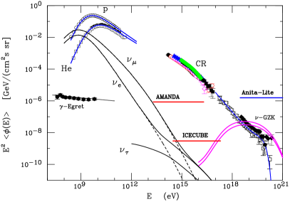
Figure 1: Neutrino fluxes. The solid lines labeled $\nu_{e}$, $\nu_{\mu}$ and $\nu_{\tau}$ show the angle averaged fluxes of atmospheric neutrinos and anti–neutrinos as a function of energy. The associated dashed lines are the fluxes neglecting the “prompt” contribution of charmed hadrons. The lines labeled $\nu$–GZK describes GZK neutrinos [6]. The points (and fitted lines) describe CR direct and indirect measurements. The horizontal lines labeled Amanda and Icecube are the current limit and the predicted sensitivity of km³ $\nu$ telescopes for an isotropic $\nu$ flux. The line labeled Anita–Lite is the limit on the $\nu$ flux obtained with radio methods [7]. The isotropic $\gamma$–ray flux measured by Egret [8] is also shown.

Figure 1 shows the angle averaged atmospheric $\nu$ fluxes [9] with an estimate of the “prompt” component [10] that “overtakes” the standard one at $E_{\nu}\sim 10$ TeV for $\nu_{e}$ and $\sim 100$ TeV for $\nu_{\mu}$.

The next two components of the neutrino fluxes are “diffuse” fluxes coming from $\nu$ production in interstellar space in our own Galaxy, and in intergalactic space. The diffuse Galactic emission is due to the interaction of cosmic rays (confined inside the Milky Way by the galactic magnetic fields) with the gas present in interstellar space. The angular distribution of this emission is expected to be concentrated in the galactic plane, very likely with a distribution similar to the one observed for GeV photons by EGRET [11]. The extragalactic diffuse emission is dominated by the decay of pions created in $p\gamma$ interactions by Ultra High Energy protons ($E_{p}\buildrel>\over{{}_{\sim}}6\times 10^{19}$ eV) interacting with the 2.7K cosmic radiation. These “GZK” neutrinos are present only at very high energy (with the flux peaking at $E_{\nu}\sim 10^{18}$ eV).

Together with the diffuse fluxes one expects the contribution of an ensemble of point–like (or quasi–point like) sources of galactic and extragalactic origin. Neutrinos travel along straight lines and allow the imaging of these sources. It is expected that most of the extragalactic sources will not be resolved, and therefore the ensemble of the extragalactic point sources (with the exception of the closest and brightest sources) will appear as a diffuse, isotropic flux that can in principle be separated from the atmospheric $\nu$ foreground because of a different energy spectrum, and flavor composition.

3 Neutrinos, Photons and Cosmic Rays

In the standard mechanism for the production of high energy $\nu$ in astrophysical sources a population of relativistic hadrons (that is cosmic rays) interacts with a target (gas or radiation fields) creating weakly decaying particles (mostly $\pi^{\pm}$, and Kaons) that produce $\nu$ in their decay. The energy spectrum of the produced neutrinos obviously reflects the spectrum of the parent cosmic rays. A well known consequence of the approximate Feynman scaling of the hadronic interaction inclusive cross sections is the fact that if the parent c.r. have a power law spectrum of form $\phi_{\rm cr}\simeq K_{\rm cr}\;E^{-\alpha}$, and their interaction probability is energy independent the $\nu$ spectrum, to a good approximation, is also a power law of the same slope.

The current favored models for 1st order Fermi acceleration of charged hadrons near astrophysical shocks predict a generated spectrum with a slope $\alpha\simeq 2$. This expectation is in fact confirmed by the observations of young SNR by HESS, and leads the expectations that astrophysical $\nu$ sources are also likely to have power law spectra with slope close to 2. Such a slope is also predicted in Gamma Rays Bursts models [20] where relativistic hadrons interact with a power law photon field. It is important to note that the high energy cutoff of the parent c.r. distribution is reflected in a much more gradual steepening of the $\nu$ spectrum for $E_{\nu}\buildrel>\over{{}_{\sim}}0.01~{}E_{p,{\rm max}}$.

The hadronic interactions that are the sources of astrophysical neutrinos also create a large number of $\pi^{\circ}$ and $\eta$ particles that decay in a $\gamma\gamma$ mode generating high energy $\gamma$–rays. In general, it is possible that these photons are absorbed inside the source, and the energy associate with them can emerge at lower frequency, however for a transparent source the relation between the photon and neutrino fluxes is remarkably robust. For a power law c.r. spectrum, the $\gamma$–rays are also created with a power law spectrum of the same slope. The approximately constant $\nu/\gamma$ ratio is shown in fig. 2 as a function of the slope $\alpha$.

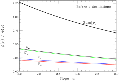
Figure 2: Ratio $\phi_{\nu}/\phi_{\gamma}$ between the neutrino and photon fluxes at $E\sim 3$ TeV, for a power law c.r. population of slope $\alpha$ and p/n ratio of 10% interacting with a low density gas target. Photon absorption is neglected. The calculation uses the Sibyll [12] hadronic interaction model. The thick line sums over all neutrino type. The $\nu$ flavor is calculated at the source before the inclusion of oscillations.

The $\nu/\gamma$ ratio is approximately constant in energy when $E$ is much smaller than the c.r. energy cutoff, and depends only weakly on the hadronic interaction model.

At the source, the relative importance of the different $\nu$ types is:

$$\{\nu_{e},\overline{\nu}_{e},\nu_{\mu},\overline{\nu}_{\mu},\nu_{\tau},\overline{\nu}_{\tau}\}~{}\simeq~{}\{1+\epsilon,1-\epsilon,2,2,0,0\}$$

where $\epsilon\sim 0.1$ depends on the slope of the spectrum, the relative importance of protons and heavy nuclei in the c.r. parent population, and the nature of the c.r. target (gas or radiation field). The ratio $\nu_{\mu}/\nu_{e}\simeq 2$ at the source is a well known consequence of the fact that the chain decay of a charged pion: $\pi^{+}\to\mu^{+}+\nu_{\mu}$ followed by $\mu^{+}\to e^{+}+\nu_{e}+\overline{\nu}_{\mu}$ generates two $\nu$ of $\mu$–flavor and one of $e$–type. The presence of a $\nu_{\mu}$ and an $\overline{\nu}_{\mu}$ in the final state insures that the ratio $\nu_{\mu}/\overline{\nu}_{\mu}\simeq 1$, while the ratio $\nu_{e}/\overline{\nu}_{e}$ is controled by the relative importance of $\pi^{+}$ over $\pi^{-}$ production that is not symmetric for a $p$ rich c.r. population.

4 Neutrino Oscillations

Measurements of solar and atmospheric neutrinos have recently established the existence of neutrino oscillations, a quantum–mechanical phenomenon that is a consequence of the non–identity of the $\nu$ flavor {$\nu_{e}$, $\nu_{\mu}$, $\nu_{\tau}$} and mass {$\nu_{1}$, $\nu_{2}$, $\nu_{3}$} eigenstates. A $\nu$ created with energy $E$ and flavor $\alpha$ can be detected after a distance $L$ with a different flavor $\beta$ with a probability that depends periodically on the ratio $L/E$. This probability oscillates according to three frequencies that are proportional to the difference between the $\nu$ squared masses $\Delta m^{2}_{jk}$, and different amplitudes related to the mixing matrix $U_{\alpha j}$ that relates the flavor and mass eigenstates. The shortest (longest) oscillation length, corresponding to the largest (smallest) $|\Delta m^{2}|$) can be written as:

$$\lambda_{12} = (4\pi\,E_{\nu})/|\Delta m^{2}_{12}|\simeq 3.1\times 10^{12}~{}E_{\rm TeV}~{}~{}{\rm cm},$$

$$\lambda_{23} = (4\pi\,E_{\nu})/|\Delta m^{2}_{23}|\simeq 0.99\times 10^{11}~{}E_{\rm TeV}~{}~{}{\rm cm}.$$

These lengths are long with respect to the Earth’s radius ($R_{\oplus}\simeq 6.371\times 10^{8}$ cm), but are very short with respect to the typical size of astrophysical sources. Therefore oscillations are negligible for atmospheric $\nu$ above $E_{\nu}\simeq 1$ TeV, but can be safely averaged for (essentially all) astrophysical neutrinos. After space averaging, the oscillation probability matrix can be written as:

$$\langle P(\nu_{\alpha}\to\nu_{\beta})\rangle = \langle P(\overline{\nu}_{\alpha}\to\overline{\nu}_{\beta})\rangle=\sum_{j}|U_{\alpha j}|^{2}\,|U_{\beta j}|^{2}$$ (1)

$$\simeq \pmatrix{0.6&0.2&0.2\cr 0.2&0.4&0.4\cr 0.2&0.4&0.4}$$

where we have used the best fit choice for the mixing parameters ($\theta_{23}=45^{\circ}$, $\theta_{12}\simeq 32.3^{\circ}$, $\theta_{13}=0$). The most important consequence of (1) is a robust prediction, valid for essentially all astrophysical sources, for the flavor composition of the observable $\nu$ signal:

$$\{\nu_{e}+\overline{\nu}_{e},\nu_{\mu}+\overline{\nu}_{\mu},\nu_{\tau}+\overline{\nu}_{\tau}\}=\{1,1,1\}$$

5 The Gamma–ray sky

The TeV energy range (the highest avaliable) for photons is the most interesting one for neutrino astronomy, because the $\nu$ signal for the future telescopes is expected to be dominated by neutrinos of one (or a few) order(s) of magnitude higher energy. Recently the new Cherenkov $\gamma$–ray telescopes have obtained remarkable results, and the catalogue of high energy gamma ray sources has dramatically increased. Of particular importance has been the scan of the galactic plane performed by the HESS telescope [13, 14], because for the first time a crucially important region of the sky has been observed with an approximately uniform sensitivity with TeV photons.

The three brightest galactic TeV sources detected by the HESS telescope have integrated fluxes above 1 TeV (in units of $10^{-11}$ (cm² s)^-1) of approximately 2.1 (CRAB Nebula), 2.0 (RX J1713.7–3946) and 1.9 (Vela Junior)

The fundamental problem in the interpretation of the $\gamma$–ray sources is the fact that it is not known if the observed photons have hadronic ($\pi^{\circ}$ decay) or leptonic (inverse Compton scattering of relativistic electrons on radiation fields) origin. If the leptonic mechanism is acting, the hadronic component is poorly (or not at all) constrained, and the $\nu$ emission can be much smaller than the $\gamma$–ray flux. For the hadronic mechanism, the $\nu$ flux is at least as large as the photon flux, and higher if the $\gamma$–rays in the source are absorbed (see sec. 3).

The $\gamma$–ray TeV sources, belong to several different classes. The Crab is a Pulsar Wind Nebula, powered by the spin down by the central neutron star. The emission from these objects is commonly attributed to leptonic processes, and in particular the Crab is well described by the Self Synchrotron Comptons model (SSC). The next two brightest sources [15, 16, 17] are young SuperNova Remnants (SNR), and there are good reasons to believe that the photon emission from these objects is of hadronic origin. The $\gamma$ spectra are power law with a slope $\alpha\simeq 2.0$–2.2 which is consistent with the expectation of the spectra of hadrons accelerated with 1st order Fermi mechanism by the SN blast wave. The extrapolation from the photon to the neutrino flux is then robust, the main uncertainty being the possible presence of a high energy cutoff in the spectrum.

Other TeV sources that are very promising for $\nu$ astronomy are the Galactic Center [18] with a measured flux $\sim 0.2$ (same units: $10^{-11}$ (cm² s)^-1) and the micro–Quasar LS5039 [19], the weakest observed TeV source with a flux $\sim 0.12$. These sources are not particularly bright in TeV $\gamma$–rays, but there are reasons to believe that they could have significant internal absorption for photons, and therefore have strong $\nu$ emission.

In general, under the hypothesis of (i) hadronic emission and (ii) negligible $\gamma$ absorption (that correspond to $\phi_{\nu}\simeq\phi_{\gamma}$), even we assume that the $\gamma$ and $\nu$ spectra extends as a power law up to 100 TeV or more, the HESS sources are just at (or below) the level of sensitivity of the new $\nu$ telescopes as will be discussed in the next section.

For extra–galactic sources the constraints from TeV photon observations are less stringent because very high energy photons are severely absorbed over extra–galactic distances due to $\gamma\gamma\to e^{+}e^{-}$ interactions on the infrared photons (from redshifted starlight) that fill intergalactic space. Active Galactic Nuclei (AGN) are strongly variables emitters of high energy radiation. The EGRET detector on the CGRO satellite has detected over 90 AGN of the Blazar class with $E_{\gamma}\geq 100$ MeV [31]. The brightest AGN sources in the present TeV $\gamma$–ray catalogue, are the nearby ($z\simeq 0.03$) AGN’s Mkn 421 and 501 that are strongly variable on all the time scales considered from few minutes to years. Their average flux can be, during some periods of time, several times the Crab. The extrapolation to the $\nu$ flux has significant uncertainties because the origin (hadronic or leptonic) of the detected $\gamma$–rays is not established.

Leading candidates as sources of high energy neutrinos are also Gamma Ray Bursts (GRB) [20, 21, 22, 23]. It is possible that individual GRB emits neutrino fluences that are sufficiently high to give detectable rates in the neutrino telescopes.

6 Point Source Sensitivity

The most promising technique for the detection of neutrino point sources is the detection of $\nu$–induced muons ($\mu\uparrow$). These particles are produced in the charged current interactions of $\nu_{\mu}$ and $\overline{\nu}_{\mu}$ in the matter below the detector. To illustrate this important point we can consider a “reference” $\nu$ point source with an unbroken power law spectrum of slope $\alpha=2.2$, and an absolute normalization (summing over all $\nu$ types) $\Phi_{\nu}(\geq 1~{}{\rm TeV})=10^{-11}$ (cm² s)^-1. The reference source flux corresponds to approximately one half the flux of the two brightest SNR detected by HESS. The event rates from the reference source of $\nu$ interactions with vertex in the detector volume, and for $\nu$–induced muons are shown in fig. 3,

Figure 3: Event rates from a $\nu$ point source. The source has spectrum $\phi_{\nu}=K\;E_{\nu}^{-\alpha}$ with slope $2.2$ and normalization $\phi_{\nu}(>1~{}{\rm TeV})=10^{-11}$ (cm² s)^-1 equaly divided among 6 $\nu$ types. The thin lines describe the rate of $\nu$–interactions in the detector volume for $e$, $\mu$ and $\tau$ like CC interactions. The thick lines are fluxes of $\nu$–induced muons with 1 GeV and 1 TeV threshold.

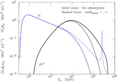
Figure 4: Event rates for $e$–like CC interactions (thin lines) and $\nu$–induced muons with a 1 GeV threshold (thick lines). The source is the same as in fig. 3). The solid (dashed) curve are for no (maximum) absorption in the Earth.

The event rates for $e$, $\mu$ and $\tau$ like $\nu$ interactions are: 10.3, 9.6 and 2.9 events/(km³ yr) (assuming a water filled volume), while the $\nu$–induced muon flux is $\phi_{\mu\uparrow}\simeq 5.6$ (km² yr)^-1. The signal depends on the zenith angle of the source, because of $\nu$ absorption in the Earth as shown in fig. 4. The rate of $e$–like events has a small contribution from the “Glashow resonance” (the process $\overline{\nu}_{e}+e^{-}\to W^{-}$), visible as a peak at $E_{\nu}\simeq m_{W}^{2}/(2m_{e})\sim 6\times 10^{6}$ GeV. Neglecting the Earth absorption the resonance contributes a small rate $\simeq 0.07$ (km³ yr)^-1 to the source signal, however this contribution quickly disappears when the source drops much below the horizon, because of absorption in the Earth.

The $\mu\uparrow$ rate is much easier to measure and to disentangle from the atmospheric $\nu$ foreground. A crucial advantage is that the detected muon allows a high precision reconstruction of the $\nu$ direction, because the angle $\theta_{\mu\nu}$ is small.

In general the relation between the neutrino and the $\nu$–induced muon fluxes is of order:

$$\Phi_{\mu\uparrow}\simeq(1\div 5)\left[{\phi_{\nu}(\geq 1~{}{\rm TeV})\over 10^{-11}~{}({\rm cm}^{2}\,{\rm s})^{-1}}\right]~{}({\rm km}^{2}\;{\rm yr})^{-1}$$ (2)

The exact relation (shown in fig. 5)

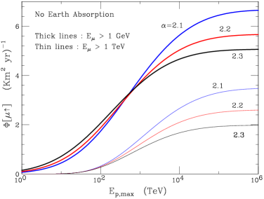
Figure 5: Flux of $\nu$–induced muons, calculated for a $\nu$ point source with a power law spectrum of slope $\alpha$, plotted as a function of the high energy cutoff of the parent proton spectrum. The thick (thin) lines are calculated for a threshold $E_{\mu{\rm min}}=1$ GeV (1 TeV). The absolute normalization is chosen so that in the absence of cutoff the total $\nu$ flux above 1 TeV has a flux $\Phi_{\nu}=10^{-11}$ (cm² s)^-1.

depends on (i) the slope of the $\nu$ spectrum, (ii) the presence of a high energy cutoff, (iii) the threshold energy used for $\mu$ detection and (iv) (more weakly) on the zenith angle of the source (because of absorption effects).

The peak of the “response” curve for the $\nu$–induced muons (see fig. 3) is at $E_{\nu}\simeq 10$ TeV (20 TeV for a threshold of 1 TeV for the muons), with a total width extending approximately two orders of magnitude. In other words the planned $\nu$ telescopes should be understood mostly as telescopes for $\simeq 10$–100 TeV neutrino sources. This energy range is reasonably well “connected” to the observations of the atmospheric Cherenkov $\gamma$-ray observations that cover the 0.1–10 TeV range in $E_{\gamma}$, and the $\nu$ sources observable in the planned km³ telescopes are likely to be appear as bright objects for TeV $\gamma$–ray instruments.

Because of the background of atmospheric muons, the $\nu$–induced $\mu$’s are only detectable when the source is below the horizon. This reduces the sky coverage of a telescope as illustrated in fig. 6, that gives the time averaged signal obtained by two detectors, placed at the south–pole and in the Mediterranean sea, when the reference source we are discussing is placed at different celestial declinations. For a south pole detector the source remains at a fixed zenith angle $\cos\theta_{\rm zenith}=-\sin\delta$, and the declination dependence of the rate is only caused by difference in $\nu$ absorption in the Earth for different zenith angles. The other curves includes the effect of the raising and setting of the source below the horizon.

Some of the most promising galactic sources are only visible for a neutrino telescope in the northern Hemisphere since the Galactic Center is at declination $\delta\simeq-29^{\circ}$. The interesting source RX J1713.7–3946 is at $\delta=-39^{\circ}$, Vela Junior at $\delta\simeq-46^{\circ}$.

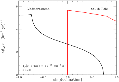
Figure 6: Average flux of up–going muons from a $\nu$ point source of fixed luminosity, plotted as a function of declination for two $\nu$ telescopes placed at the south pole (thick line) and in the mediterranean sea (thin line). The flux is considered detectable only when the source is below the horizon. The effects of the (variable) absorption in the Earth is taken into account.

6.1 Background Estimates

Since the prediction of the signal size for from the (expected) brightest $\nu$ sources is of only few events per year, it is clearly essential to reduce all sources of background to a very small level. This is a possible but remarkably difficult task.

The background problem is illustrated in fig. 7 that shows the energy spectrum of the muon signal from our “reference” point source, comparing it with the spectrum of the atmospheric $\nu$ foreground integrated in a small cone of semi–angle 0.3^∘. The crucial point is that the energy spectrum from astrophysical sources is harder than the atmospheric $\nu$ one, with a median energy of approximately 1 TeV, an order of magnitude higher. It is for this reason that for the detection of astrophysical neutrinos it is planned to use an “offline” threshold of $E_{\mu}\buildrel>\over{{}_{\sim}}1$ TeV. The atmospheric background above this threshold is small but still potentially dangerous, it depends on the zenith angle and is maximum (minimum) for the horizontal (vertical) direction at the level of 4 (1) $\mu$/(km² yr).

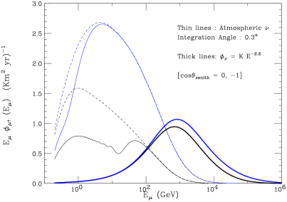
Figure 7: Energy Spectra of $\nu$–induced muons. The thin lines are the atmospheric $\nu$ background integrated in a cone of semi–angle $0.3^{\circ}$ (dashed lines do not consider oscillations). The thick lines are for a point source ($\alpha=2.2$, $\phi_{\nu}(>1~{}{\rm TeV})=10^{-11}$ (cm² s)^-1. The high (low) line is for horizontal (vertical) muons.

The angular window for the integration of the muon signal is determined by three factors: (i) the angular shape of the source, (ii) the intrinsic angle $\theta_{\mu\nu}$, and (iii) the angular resolution of the instrument. The source dimension can be important for the galactic sources, in fact the TeV $\gamma$–ray sources have a finite size, in particular the SNR RX J1713.7–3946 has a radius $\sim 1^{\circ}$, and Vela Junior is twice as large. The detailed morphology of these sources measured by the HESS telescope indicates that most of the emission is coming from only some parts of the shell (presumably where the gas density is higher), and the detection of $\nu$ emission from these sources could require the careful selection of the angular region of the $\gamma$–ray signal.

The distribution of the $\theta_{\mu\nu}$ angle defines the minimum angular dimension of a perfect point source signal. This is shown in fig. 8 that plots the semi–angle of the cone that contains 50, 75 or 90% of such a signal (for a $\alpha=2.2$ spectrum) as a function of the muon energy. The size the muon signal shrinks with increasing energy $\propto(E_{\mu})^{-1/2}$. This is easily understood noting that the dominant contribution to $\theta_{\mu\nu}$ is the muon–neutrino scattering angle at the $\nu$–interaction point:

$$\cos\theta_{\mu\nu}=1-\frac{m_{N}\,x}{E_{\mu,0}}~{}\left(1-\frac{E_{\mu,0}}{E_{\nu}}\right)$$ (3)

($E_{\mu,0}$ is the muon energy at the interaction point), and expanding for small angle one finds $\theta_{\mu\nu}\sim\sqrt{m_{N}\,x/(2\,E_{\mu,0})}$.

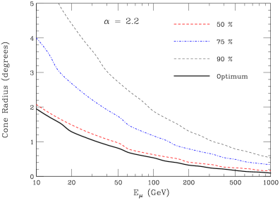
Figure 8: Angular distribution of the upgoing muon flux induced by a $\nu$ power law flux of slope $\alpha=2.2$. The curves give the semi–angle angle of the cone that (for a fixed value of $E_{\mu}$) contains 50%, 75% and 90% of the signal. The thick line gives the cone that maximize the $S/\sqrt{B}$.

The 50% containement cone angle shrinks to $\theta_{50\%}\simeq 0.15^{\circ}$ for $E_{\mu}=1$ TeV that is probably smaller than the experimental resolution.

Qualitatively the experimental strategy for the maximization of the point–source sensitivity is clear: (i) selection of high energy $E_{\mu}\buildrel>\over{{}_{\sim}}1$ TeV muons, and (ii) selection of the narrowest angular window compatible with the experimental resolution and the signal angular size. These cuts will reduce the total signal by at least a factor of 2. The optimization of the cuts for signal extraction is a non–trivial problem, that we cannot discuss here. In principle one would like to maximize the quantity $S/\sqrt{B}$ (where $S$ and $B$ are respectively the signal and background event numbers). For the angular window (where $B\propto\theta$) this problem has a well defined solution that is shown in fig. 8, that corresponds to the choice of a window that contains approximately 50% of the signal. This is the numerically obtained generalization of the well known fact that for a gaussian angular resolution of width $\sigma_{\theta}$, $S/\sqrt{B}$ is maximized choosing the angular window $\theta\leq 1.585\,\sigma_{\theta}$ that contains a fraction 0.715 of the signal. For the energy cut, the quantity $S/\sqrt{B}$ grows monotonically when the threshold energy is increased, and therefore the optimum is determined by the condition that the background approaches zero.

6.2 Sensitivity and Sources

The conclusion of this discussion on the point–source sensitivity is that after careful work for background reduction, the minimum $\nu$ flux (above 1 TeV) detectable as a point source for the km³ telescopes is of order (or larger than) $\Phi_{\nu}\sim 10^{-11}$ (cm² s)^-1, that is approximately the $\nu$ flux of the reference source considered above. This is tantalizingly (and frustratingly) close to the flux predicted from the extrapolation (performed under the assumption of a transparent source) of the brightest sources in the TeV $\gamma$–ray catalogue.

The remarkable recent results of HESS and MAGIC on galactic sources are certainly very exciting for the $\nu$ telescope builders, because they show the richness of the “high energy” sky, but they are also sobering, because they lead to a prediction of the scale of the brightest galactic $\nu$ sources, that is just at the limit of the sensitivity of the planned instruments. As discussed previously, strong $\nu$ sources could lack a bright $\gamma$–ray counterparts because of internal photon absorption, or because they are at extra–galactic distances.

The considerations outlined in this section can be immediately applied to a burst–like transient sources like GRB’s. In the presence of a photon “trigger” that allows a time coincidence, the background problem disappears and the detectability of one burst is only defined by the signal size. A burst with an $\nu$ energy fluence $F_{\nu}\simeq 2\times 10^{-4}$ erg/cm² per decade of energy (in the 10–100 TeV range) will produce an average of one $\nu$–induced muon in a km³ telescope.

7 Extragalactic Neutrino Sources

The flux from the ensemble of all extragalactic sources, with the exception of a few sources will appear as an unresolved isotropic flux, characterized by its energy spectrum $\phi(E)$. The identification of this unresolved component can rely on three signatures: (i) an energy spectrum harder that the atmospheric flux, (ii) an isotropic angular distribution, and (iii) approximately equal fluxes for all 6 neutrino types. This last point is a consequence of space averaged flavor oscillations.

The flux of prompt (charm decay) atmospheric neutrinos is also approximately isotropic in the energy range considered, and is characterized by equal fluxes of $\nu_{e}$ and $\nu_{\mu}$, with however a significant smaller flux of $\nu_{\tau}$ (that are only produced in the decay of $D_{s}^{\pm}$). The disentangling of the astrophysical and an prompt–atmospheric fluxes is therefore not trivial, and depends on a good determination of the neutrino energy spectrum, together with a convincing model for charmed particle production in hadronic interactions. A model independent method for the identification of the astrophysical flux requires the separate measurement of the fluxes of all three neutrino flavors, including the $\nu_{\tau}$. The flux of prompt atmospheric $\nu_{\mu}$ is also accompanied by an approximately equal flux of $\mu^{\mp}$ (the differences at the level of 10% are due to the very well understood differences in the spectra produced in weak decays). The down–going muon flux is in principle measurable, determining the prompt component experimentally and eliminating a potentially dangerous background. This measurement is therefore important and efforts should be made to perform it.

7.1 Energetics of Extra–galactic neutrinos

The most transparent way to discuss the $\nu$ extragalactic flux is to consider its energetics. The observable $\nu$ flux $\phi(E)$ is clearly related to a number density $n(E)=(4\pi/c)\,\phi(E)$ and to an energy density $\rho(E)=E\,n(E)$, that fill uniformly the universe. The $\nu$ energy density at the present epoch has been generated by a power source acting during the history of the universe. Integrating over all $E_{\nu}$, the relation between the power injection density $\mathcal{L}(t)$ and the $\nu$ energy density at the present epoch is given by:

$$\rho_{\nu} = \int_{0}^{t_{0}}\;dt~{}{\mathcal{L}(t)\over[1+z(t)]}~{}=~{}\int_{0}^{\infty}\;dz~{}\left|{dt\over dz}\right|~{}{\mathcal{L}(z)\over(1+z)}$$ (4)

$$= \int_{0}^{\infty}\;dz~{}{\mathcal{L}(z)\over H(z)\;(1+z)^{2}}~{}=~{}{\mathcal{L}_{0}\over H_{0}}~{}\xi$$

where $t_{0}$ is the age of the unverse, $\mathcal{L}_{0}$ and $H_{0}$ are the $\nu$ power density and the Hubble constant at the present epoch, and $\xi$ is the adimensional quantity:

$$\xi=\int_{0}^{\infty}\,dz~{}\left[\frac{H_{0}}{H(z)}\right]~{}\left[\frac{\mathcal{L}(z)}{\mathcal{L}_{0}}\right]\;(1+z)^{-2}~{}~{}.$$ (5)

that depends on the cosmological parameters, and more crucially on the cosmic history of the neutrino injection. The quantity $\mathcal{L}_{0}\,\xi$ can be understood as the effective “average power density” operating during the Hubble time $(H_{0})^{-1}$, and depends on the cosmological parameters, and more strongly on the cosmological history of the injection. For a Einstein–De Sitter universe ($\Omega_{\rm m}=1$, $\Omega_{\Lambda}=0$) with no evolution for the sources one has $\xi=0.4$, for the “concordance model” cosmology ($\Omega_{\rm m}=0.3$, $\Omega_{\Lambda}=0.7$) this becomes $\xi=0.53$. For the same concordance model cosmology, if it is assumed that the cosmic time dependence of the neutrino injection is similar to the one fitted to the star–formation history [25, 26], one obtains $\xi({\rm SFR})\simeq 3.0$, for a time dependence equal to the one fitted to the AGN luminosity evolution [27] one finds $\xi({\rm AGN})\simeq 2.2$.

If we consider the power and energy density not bolometric, but only integrated above the threshold energy $E_{\rm min}$, the redshift effects depend on the shape of the injection spectrum. For a power law of slope $\alpha$ independent from cosmic time, one has still a relation of form:

$$\rho_{\nu}(E_{\rm min})=\frac{\mathcal{L}_{0}(E_{\rm min})}{H_{0}}~{}\xi_{\alpha}$$ (6)

very similar to (4), with:

$$\xi_{\alpha}=\int_{0}^{\infty}\,dz~{}\left[\frac{H_{0}}{H(z)}\right]~{}\left[\frac{\mathcal{L}(z)}{\mathcal{L}_{0}}\right]\;(1+z)^{-\alpha}$$ (7)

For $\alpha=2$ one has $\xi_{2}=\xi$. The energy density (6) corresponds to the $\nu$ isotropic differential flux:

$$\phi_{\nu}(E) = K_{\nu}~{}E^{-\alpha}$$ (8)

$$= \left(\frac{\mathcal{L}_{0}(E_{\rm min})\,E_{\rm min}^{\alpha-2}\,\xi_{\alpha}\,k_{\alpha}}{4\pi\,H_{0}}\right)~{}E^{-\alpha}$$

where $k_{\alpha}$ is the kinematic adimensional factor:

$$k_{\alpha}\simeq(\alpha-2)/[1-(E_{\rm min}/E_{\rm max})^{\alpha-2}]^{-1}$$ (9)

with $E_{\rm max}$ the high energy cutoff of the spectrum. The limit of $k_{\alpha}$ when $\alpha\to 2$ is: $k_{\alpha}=\left[\log(E_{\rm max}/E_{\rm min})\right]^{-1}$. One can use equation (8) to relate the observed diffuse $\nu$ flux to the (time and space) averaged power density of the neutrino sources:

$$(K_{\nu}\;E_{\rm min}^{2-\alpha})=\frac{\mathcal{L}_{0}(E_{\rm min})~{}\xi_{\alpha}~{}k_{\alpha}}{4\pi\;H_{0}}$$ (10)

The case $\alpha=2$ corresponds to an equal power emitted per energy decade, and numerically:

$$K_{\nu}\simeq 3.7\times 10^{-11}~{}\left[\frac{(\mathcal{L}_{0}\,\xi)_{\rm decade}}{L_{\odot}/{\rm Mpc}^{3}}\right]~{}\frac{\rm GeV}{{\rm cm}~{}{\rm s}~{}{\rm sr}}$$ (11)

($L_{\odot}$ is the solar luminosity). The current limit on the existence of a diffuse, isotropic $\nu$ flux of slope $\alpha\simeq 2$ from the AMANDA and Baikal detectors corresponds to $K_{\nu}\buildrel<\over{{}_{\sim}}8\times 10^{-7}$ GeV/(cm² s sr)^-1, while the sensitivity of the future km³ telescopes is estimated (in the same units) of order $K_{\nu}\sim 3\times 10^{-9}$. This implies that the average power density for the creation of high energy neutrinos is:

$$(\mathcal{L}_{0}\xi)\buildrel<\over{{}_{\sim}}2.4\times 10^{4}~{}\left(L_{\odot}~{}{\rm Mpc}^{-3}\right)~{}{\rm decade}^{-1}$$ (12)

the future km³ telescopes will detect the extragalactic flux if it has been generated with an “average” power density $(\mathcal{L}_{0}\,\xi)\buildrel>\over{{}_{\sim}}80$ (same units).

7.2 Possible Sources of Power

To evaluate the astrophysical significance of the current limits on the diffuse $\nu$ flux and of the expected sensitivity of the km³ telescopes, one can consider the energetics of the most plausible sources of high energy neutrinos, namely the death of massive stars and the activity around Super Massive Black Holes at the center of galaxies.

7.2.1 The Death of Stars

The bolometric average power density associated with stellar light has been estimated by Hauser and Dwek [28] as:

$$(\mathcal{L}\,\xi_{\rm star})^{\rm bol}=(0.36\div 1.23)\times 10^{9}\left(L_{\odot}~{}{\rm Mpc}^{-3}\right)$$ (13)

this is also in good agreement with the estimate of Fukugita and Peebles [26] for the B–band optical luminosity of stars. This power implies that the total mass density gone into the star formation [26] is:

$$\rho_{\rm star}\simeq 5.9\times 10^{8}~{}\left({M_{\odot}~{}{\rm Mpc}^{-3}}\right)$$ (14)

(that implies $\Omega_{\rm star}=0.0043\simeq 0.09\;\Omega_{\rm baryon}$). Most of this power has of course little to do with cosmic rays and high energy $\nu$ production, however c.r. acceleration has been associated with the final stages of the massive stars life. A well established mechanism is acceleration in the spherical blast waves of SuperNova explosions, a more speculative one is acceleration in relativistic jets that are emitted in all or a subclass of the SN, and that is the phenomenon behind the (long duration) Gamma Ray Bursts. The current estimate of the rate of gravitational collapse supernova rate obtained averaging over different surveys [26] is:

$$R_{\rm SN}^{\rm observed}\simeq 7.6^{+6.4}_{-2.0}\times 10^{-4}~{}({\rm Mpc}^{3}~{}{\rm yr})^{-1}$$ (15)

This is reasonably consistent with the the estimate of the power emitted by stars, if one assumes that all stars with $M>8~{}M_{\odot}$ end their history with a gravitational collapse. Fukugita and Peebles estimate ($\psi(0)$ is the SFR at thre present epoch):

$$R_{\rm SN} = \psi(0)~{}{\int_{8}^{100}~{}dM~{}{dN\over dM}\over\int_{0.08}^{100}~{}dM~{}M~{}{dN\over dM}}$$ (16)

$$\simeq 7.9^{+2.4}_{-3.9}\times 10^{-4}~{}({\rm Mpc}^{3}~{}{\rm yr})^{-1}$$

Assuming that the average kinetic energy released in a SN explosion is of order $\langle E_{\rm kin}\rangle_{SN}\simeq 1.6\times 10^{51}~{}{\rm erg}$ this implies an average power density:

$$\left(\mathcal{L}\;\xi\right)_{{\rm SN},{\rm kin}}\simeq 4.2\times 10^{6}~{}\left(L_{\odot}~{}{\rm Mpc}^{-3}\right)$$ (17)

It is commonly believed that a fraction of order $\sim 10$% of this kinetic energy is converted into relativistic hadrons. One can see that if on average a fraction of order 1% is converted in neutrinos, this could result in $(\mathcal{L}_{0}\,\xi)_{\nu}\sim 10^{3}~{}\left(L_{\odot}~{}{\rm Mpc}^{-3}\right)$, that could give a a detectable signal from the ensemble of ordinary galaxies.

7.2.2 Active Galactic Nuclei

Active Galactic Nuclei have often been suggested as a source of Ultra High energy Cosmic Rays, and at the same time of high energy neutrinos. Estimates of the present epoch power density from AGN in the [2,10 KeV] $X$–ray band are of order

$$\mathcal{L}_{0,{\rm AGN}}^{[2,10\,{\rm KeV}]}\simeq 2.0\times 10^{5}~{}\left(L_{\odot}~{}{\rm Mpc}^{-3}\right)$$ (18)

with a cosmic evolution [27] characterized by $\xi\sim 2.2$. Ueda [27] also estimates the relation between this energy band and the bolometric luminosity is: $L_{\rm bol}\simeq 30~{}L_{X}^{[2,10\,{\rm KeV}]}.$ and therefore the total power associated with AGN is

$$\left(\mathcal{L}\,\xi\right)_{\rm AGN}^{\rm bol}\simeq 10^{7}~{}\left(L_{\odot}~{}{\rm Mpc}^{-3}\right)$$ (19)

of order $\sim 1$% of the power associated with star light. It is remarkable that this AGN luminosity is well matched to the average mass density in Super Massive Black Holes, that is estimated [29, 30]:

$$\rho_{\bullet}=4.6^{+1.9}_{-1.4}\times 10^{5}~{}M_{\odot}~{}{\rm Mpc}^{-3}$$ (20)

When a mass $m$ falls into a Black Hole (BH) of mass $M_{\bullet}$ the BH mass is increased by an amount: $\Delta M_{\bullet}=(1-\varepsilon)\,m$ while the energy $\varepsilon\,m$ is radiated away in different forms. The total accreted mass can therefore be related to the amount of radiated energy, if one knows the radiation efficiency $\varepsilon$:

$$M_{\bullet}={(1-\varepsilon)\over\varepsilon}~{}E_{\rm radiated}$$ (21)

and therefore

$$\rho_{\bullet}=(\mathcal{L}\,\xi)_{\rm AGN}~{}H_{0}^{-1}\frac{1-\varepsilon}{\varepsilon}$$ (22)

The estimates (19) and (20) are consistent for an efficiency $\varepsilon\simeq 0.1$. Assuming radiated energy is the kinetic energy accumulated in the fall down to a radius $r$ that is $f$ times the BH Schwarzschild radius $R_{S}=2G\,M_{\bullet}$:

$$\varepsilon={E_{\rm radiated}\over m}\simeq{G\,M_{\bullet}\over f\,R_{S}}={1\over 2\,f}$$ (23)

this corresponds to $f\sim 5$.

The ensemble of AGN has sufficient power to generate a diffuse $\nu$ flux at the level of the existing limit.

7.3 Gamma Ray Bounds

A very important guide for the expected flux of extragalactic $\nu$ is the diffuse $\gamma$–ray flux measured above 100 MeV measured by the EGRET instrument [8] that can be described (integral flux above a minimum energy $E_{\gamma}$ in GeV) as:

$$\Phi_{\gamma}(E_{\gamma})\simeq 1.42\times 10^{-6}E_{\gamma}^{-1.1}({\rm cm}^{2}\,{\rm s}\,{\rm sr})^{-1}$$ (24)

(for a critical view of this interpretation see [32]). This corresponds to the energy density in the decade between $E_{\gamma}$ and $10\,E_{\gamma}$ (with $E_{\gamma}$ in GeV): $\rho_{\gamma}(E_{\gamma})\simeq 1.35\times 10^{-6}~{}E_{\rm min}^{-0.1}\,{\rm eV}~{}{\rm cm}^{-3}$ and to the average power density per decade:

$$\left(\mathcal{L}\;\xi\right)_{\gamma}\simeq 3.7\times 10^{4}~{}{E_{\gamma}}^{-0.1}~{}\left(L_{\odot}~{}{\rm Mpc}^{-3}\right)$$ (25)

This diffuse $\gamma$–ray has been attributed [33] to the emission of unresolved Blazars. The sum of the measured fluxes (for $E_{\gamma}>100$ MeV) for all identified EGRET blazars [31] amounts to: $\sum_{{\rm Blazars}}\phi_{j}\simeq 0.33~{}({\rm m}^{2}\,{\rm s})^{-1}$ This has to be compared with the diffuse flux (24) that can be re-expressed as: $4\pi\;\Phi_{\gamma}(100~{}{\rm MeV})\simeq 2.62~{}({\rm m}^{2}\,{\rm s})^{-1}$. Other authors [34] arrive to the interesting conclusion that unresolved blazars can account for at most 25% of the diffuse flux, and that there must be additional sources of GeV photons.

Most models for the Blazar emission favor leptonic mechanism, with the photons emitted by the Inverse Compton scattering of relativistic electrons with radiation fields present in the jet, however it is possible that hadrons account for a significant fraction (or even most) of the $\gamma$–ray flux, and therefore that the $\nu$ flux is of comparable intensity to the $\gamma$ flux. The test of the “Egret level” for the diffuse $\nu$ flux is one of the most important goals for the neutrino telescopes already in operation.

7.4 Cosmic Rays Bounds

Waxman and Bahcall [35] have suggested the existence of an upper bound for the diffuse flux of extra–galactic neutrinos that is valid if the $\nu$ sources are transparent for cosmic rays, based on the observed flux of ultra high energy cosmic rays. The logic (and the limits) of the WB bound are simple to grasp. Neutrinos are produced by cosmic ray interactions, and it is very likely (and certainly economic) to assume that the c.r. and $\nu$ sources are the same, and that the injection rates for the two type of particles are related. The condition of “transparency” for the source means that a c.r. has a probability $P_{\rm int}\buildrel<\over{{}_{\sim}}0.5$ of interacting in its way out of the source. The transparency condition obviously sets an upper bound on the $\nu$ flux, that can be estimated from a knowledge of the cosmic ray extragalactic spectrum, calculating for each observed c.r. the spectrum of neutrinos produced in the shower generated by the interaction of one particle of the same mass and energy, and integrating over the c.r. spectrum. If the c.r. spectrum is a power law of form $\phi_{\rm c.r.}(E)=K\;E^{-\alpha}$, the “upper bound” $\nu$ flux obtained saturating the transparency condition (for a c.r. flux dominated by protons) is: $\phi_{\nu}=(K\,Z_{p\to\nu})\;E^{-\alpha}$ with $Z_{p\to\nu}\sim 0.25$

The WB upper bound (shown in fig. 9) has been the object of several criticisms see for example [36]. There are two problems with it. The first one is conceptual: the condition of transparency is plausible but is not physically necessary. The c.r. sources can be very transparent, for example in SNR’s the interaction probability of the hadrons accelerated by the blast wave, is small ($\ll 1\%$) (with a value that depends on the density of the local ISM), but “thick sources” are possible, and have in fact been advocated for a long time, the best example is acceleration in the vicinity of the horizon of a SMBH. The search for “thick” neutrino sources is after all one of the important motivations for $\nu$ astronomy.

The second problem is only quantitative. In order to estimate the bound one has to know the spectrum of extra–galactic cosmic rays. This flux is “hidden” behind the foreground of galactic cosmic rays, that have a density enhanced by magnetic confinement effects.

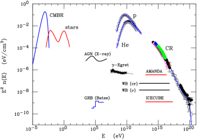
Figure 9: Different contributions to the average energy density in the universe. Different lines describe the contributions of the 2.7^∘ K CMBR radiation, starlight (with reprocession by dust), the X-ray diffuse flux (attributable to AGN, the Egret ($E_{\gamma}\geq 100$ MeV) diffuse flux, and the GRB contribution from the BATSE data. The detected cosmic ray energy density (points) is enhanced by magnetic confinement in our galaxy and is not cosmological, except (possibly) at the highest energy. The lines labeled WB(cr) and WB($\nu$) are the extragalactic c.r. and upper bound $\nu$ fluxes estimated in [35]. The line labeled Amanda is the current limit on an isotropic extragalactic $\nu$ flux, and the line labeled ICECUBE is the predicted sensitivity on km³ telescopes.

The separation of the galactic and extragalactic component of the c.r. is a central unsolved problem for cosmic ray science. The extragalactic c.r. is dominant and therefore visible only at the very highest energies, perhaps only above the “ankle” (at $E_{\rm ankle}\simeq 10^{19}$ eV) as assumed in [35]. More recently it has been argued [37] that extra–galactic $p$ dominate the c.r. flux for $E_{0}\buildrel>\over{{}_{\sim}}10^{18}$ eV. Waxman and Bahcall have fitted the c.r. flux above the ankle with an a $E^{-2}$ injection spectrum (correcting for energy degradation in the CMBR) and extrapolated the flux with the same form to lower energy. The power needed to generate this c.r. density was $\mathcal{L}_{\rm cr}\simeq 1900~{}L_{\odot}/$(Mpc³ decade). The extrapolation of the c.r. flux (that is clearly model dependent) and the corresponding $\nu$ upper bound are shown in fig. 9, where they can be compared to the sensitivity of the $\nu$ telescopes.

Because of the uncertainties in the fitting of the c.r. extragalactic component and its extrapolation to low energy (and the possible loophole of the existence of thick souces) the WB estimate cannot really be considered an true upper bound of the $\nu$ flux. However the “WB $\nu$–flux” is important as reasonable (and indeed in many senses optimistic) estimate of the order of magnitude of the true flux. The existence of cosmic rays with energy as large as $E_{0}\sim 10^{20}$ eV is the best motivation for neutrino astronomy, since these particles must be accelerated to relativistic energies somewhere in the universe, and unavoidably some c.r. will interact with target near (or in) the source producing neutrinos.

7.5 Resolved and Unresolved Fluxes

An interesting question is the relation between the intensity of the total extragalactic $\nu$ contribution, and the potential to identify extra–galactic point sources. This clearly depends on the luminosity function and cosmological evolution of the sources. Assuming for simplicity that all sources have energy spectra of the same shape, and in particular power spectra with slope $\alpha$, then each source can be fully described by its distance and its $\nu$ luminosity $L$ (above a fixed energy threshold $E_{\rm min}$). The ensemble of all extra–galactic sources is then described by the function $n(L,z)\,dL$ that gives the number of sources with luminosity in the interval between $L$ and $L+dL$ contained in a unit of comoving volume at the epoch corresponding to redshift $z$. The power density due to the ensemble of all sources is given by:

$$\mathcal{L}(z)=\int dL~{}L~{}n(L,z)$$ (26)

It is is possible (and in fact very likely) that most high energy neutrino sources are not be isotropic. This case is however contained in our discussion if the luminosity $L$ is understood as an orientation dependent “isotropic luminosity”: $L\equiv(4\pi)\,(dL_{\rm true}/d\Omega)$. For a random distribution of the viewing angles it is easy to show that

$$\int dL~{}L~{}n(L,z)=\int dL_{\rm true}~{}L_{\rm true}~{}n(L_{\rm true},z)$$ (27)

The $\nu$ flux (above the threshold energy $E_{\rm min}$) received from a source described by $L$ and $z$ is:

$$\Phi_{\rm point}(L,z)=\frac{L}{4\pi\;E_{\rm min}}~{}\frac{k_{\alpha}}{(\alpha-1)}~{}\frac{(1+z)^{2-\alpha}}{d_{L}(z)^{2}}$$ (28)

where $d_{L}(z)$ is the luminosity distance and $k_{\alpha}$ is the adimensional factor given in (9).

If $\Phi_{\rm min}$ is the sensitivity of a neutrino telescope, that is the minimum flux for the detection of a point source, then a source of luminosity $L$ can be detected only if is closer than a maximum distance corresponding to redshift $z_{h}(L)$. Inspecting equation (28) it is simple to see that $z_{h}$ is a function of the adimensional ratio $x=\sqrt{L/L^{*}}$ where:

$$L^{*}=4\pi\,E_{\rm min}\,\Phi_{\rm min}~{}(\alpha-1)/(H_{0}^{2}\;k_{\alpha})$$ (29)

is the order of magnitude of the luminosity of a source that gives the minimum detectable flux when placed at $z\sim 1$. The explicit solution for $z_{h}(x)$ depends on the cosmological parameters ($\Omega_{\rm m}$, $\Omega_{\Lambda}$) and on the spectral slope $\alpha$. A general closed form analytic solution for $z_{h}(x)$ does not exist, but it can be easily obtained numerically. The solution for the concordance model cosmology is shown in fig. 10.

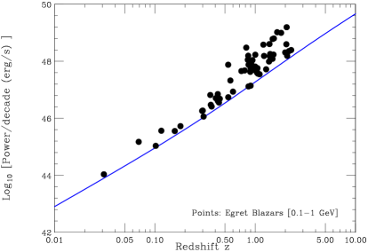
Figure 10: Redshift horizon $z_{h}(L)$ calculated for the cosmology $\Omega_{\rm m}=0.3$, $\Omega_{\Lambda}=0.7$, and sources with power law spectra of slope $\alpha=2$, assuming the a minimum detectable flux $\Phi_{\nu}(\geq 1~{}{\rm TeV}=10^{-11}$ (cm²s)^-1. The points corresponds to the EGRET blazars [31] with the luminosity measured in the 0.1–10 GeV range.

It is also easy and useful to write $z_{h}$ as a power law expansion in $x$:

$$z_{h}=x+\frac{1}{4}\left[2(1-\Omega_{\Lambda})+\Omega_{\rm m}-2\alpha\right]\,x^{2}+\ldots$$ (30)

The leading term of this expansion is simply $x$ independently from the cosmological parameters and the slope $\alpha$. This clearly reflects the fact that for small redshift $z$ one probes only the near universe, where and when redshift effects and cosmological evolution are negligible, and the flux simply scales as the inverse square of the distance.

The total flux from all (resolved and unresolved) sources can be obtained integrating over $L$ and $z$:

$$\Phi_{\rm tot}=\frac{1}{4\pi}\int dL\int_{0}^{\infty}dz\;v(z)\,n(L,z)\;\Phi_{\rm point}(L,z)$$ (31)

where $v(z)$ is the comoving volume contained between redshift $z$ and $z+dz$:

$$v(z)=4\pi\;~{}\frac{d_{L}^{2}(z)}{(1+z)^{2}\;{H}(z)}\simeq\frac{4\pi}{H_{0}^{2}}\,z^{2}\,(1+\ldots)$$ (32)

Substituting the definitions (28) and (32), integrating in $L$ and using (26) the total flux corresponds exactly to the result (8). The resolved (unresolved) flux can be obtained changing the limits of integration in redshift to the interval $z\in[0,z_{h}(L)]$ ($z\in[z_{h}(L),\infty]$). The total number of detectable sources is obtained integrating the source density in the comoving volume contained inside the horizon:

$$N_{\rm s}=\int dL~{}\int_{0}^{z_{h}(L)}dz~{}v(z)~{}n(L,z)$$ (33)

A model for $n(L,z)$ to describe the luminosity distribution and cosmic evolution of the sources allows to predict the fraction of the extra–galactic associated with the resolved flux, and the corresponding number of sources. Here there is no space for a full discussion, but it may be instructive to consider a simple toy model where all sources have identical luminosity (that is $n(L,z)=n\;\delta[L-\overline{L}(z)]$). In this model, is the (unique) luminosity $L$ of the sources at the present epoch is not too large, (that is for $L\buildrel<\over{{}_{\sim}}L^{*}$ with $L^{*}$ given in (29)), for a fixed total flux for the ensemble of sources, the number of objects that can be resolved is (for $\alpha\simeq 2$):

$$N_{\rm s} ~{}\simeq~{} \frac{\sqrt{4\pi}}{3}\,\frac{1}{\xi~{}\log(10)}\;\frac{H_{0}}{c}\frac{K_{\nu}\,\sqrt{L_{\rm decade}}}{(\Phi_{\rm min}~{}E_{\rm min})^{3/2}}$$ (34)

$$~{}\simeq~{} 10~{}\left(K_{-9}\right)\,\left(\Phi^{\rm min}_{-11}\right)^{-\frac{3}{2}}\,\left(L_{45}\right)^{\frac{1}{2}}\,\frac{2.5}{\xi}$$

where $K_{\nu}$ is the coefficient of the diffuse $\nu$ flux ($K_{-9}$ is in units $10^{-9}$ GeV/(cm² s sr)), $L_{\rm dec}$ is the power of an individual source per energy decade ($L_{45}$ is in units of $10^{45}$ erg/s), and $\Phi_{\rm min}$ is the minum flux above energy $E_{\rm min}=1$ TeV for source identification ($\Phi_{-11}$ is in units $10^{-11}$ (cm²s)^-1). It is easy to understand the scaling laws. When the luminosity of the source increases the radius of the source horizon (for $L$ not too large) grows $\propto\sqrt{L/\Phi_{\rm min}}$ and the corresponding volume grows as $V\propto(L/\Phi_{\rm min})^{3/2}$, while (for a fixed total flux) the number density of the sources is $n\propto K_{\nu}\,L^{-1}$, therefore the number of detectable sources is: $N_{\rm s}\propto n\,V\propto K_{\nu}\;L^{1/2}\;\Phi_{\rm min}^{-3/2}$.

Similarly, the ratio of the resolved to the total $\nu$ flux can be estimated as:

$$\frac{\phi_{\rm resolved}}{\phi_{\rm total}} \simeq \frac{1}{4\pi}~{}\frac{1}{\xi~{}\log(10)}~{}\frac{H_{0}^{2}}{c^{2}}~{}\frac{L_{\rm dec}}{\Phi_{\rm min}~{}E_{\rm min}}$$ (35)

$$\simeq 0.005~{}~{}\left(\Phi^{\rm min}_{-11}\right)^{-1}~{}\left(L_{45}\right)\,\frac{2.5}{\xi}$$ (36)

The scaling $\propto L/\Phi_{\rm min}$ also easily follows from the assumption of an euclidean near universe.

The bottom line of this discussion, is that it is very likely that the ensemble of all extra–galactic sources will give its largest contribution as an unresolved , isotropic contribution, with only a small fraction of this total flux resolved in the contribution of few individual point sources. The number of the detectable extra–galactic point sources will obviously grow linearly with total extra–galactic flux, but also depends crucially on the luminosity function and cosmological evolution of the $\nu$ sources. If a reasonable fraction of the individual sources are sufficiently powerful ($L\buildrel>\over{{}_{\sim}}10^{45}$ erg/s), an interesting number of objects can be detected as point sources. Emission for blazars is a speculative but very exciting possibility (see fig. 10).

8 GZK neutrinos

For lack of space we cannot discuss here the neutrinos of “GZK” origin and other speculative sources [38]. This field is of great interest, and is in many ways complementary to the science that can be performed with km³ telescopes. GZK neutrinos (see fig.1) have energy typically in the 10¹⁸–10²⁰ eV, and the predicted fluxes are so small that km³ detectors can only be very marginal, and larger detector masses and new detection methods are in order. Several interesting ideas are being developed (for a review see [39]), these include acoustic [40], radio [41] and Air Shower [42, 43] detection.

The GZK neutrinos are a guaranteed source, and their measurement carry important information on the maximum energy and cosmic history of the ultra high energy cosmic rays. Perhaps the most promising detection technique uses radio detectors on balloons. An 18.4 days test flight of the ANITA experiment [7] (see fig. 1) has obtained the best limits on the diffuse flux of neutrinos at very high energy.

As photon astronomy is articulated in different fields according to the range of wavelength observed, for neutrino astronomy one can already see the formation of (at least) two different subfields: the “km³ neutrino Science” that aims at the study of $\nu$ in the 10¹²–10¹⁶ eV energy range, and “Ultra High Energy neutrino Science” that studies $\nu$ above 10¹⁸ eV, with the detection of GZK neutrinos as the primary goal.

9 Conclusions and Outlook

The potential of the km³ telescopes to open the extraordinarily interesting new window of high energy neutrino astronomy is good. The closest thing to a guaranteed $\nu$ source are the young SNR observed by HESS in TeV photons. The expected $\nu$ fluxes from these sources are probably above the sensitivity of a km³ telescopes in the northern hemisphere. Other promising galactic $\nu$ sources are the Galactic Center and $\mu$Quasars. Blazars and GRB’s are also intensely discussed as extragalactic $\nu$ sources. The combined $\nu$ emission of all extragalactic sources should also be detectable as a diffuse flux distinguishable from the atmospheric $\nu$ foreground. Because of the important astrophysical uncertainties, the clear observations of astrophysical neutrinos in the km³ telescopes is however not fully guaranteed.

There are currently plans to build two different instruments of comparable performances (based on the water Cherenkov technique in water and ice) in the northern and southern hemisphere. Such instruments allow a complete coverage of the celestial sphere. This is a very important scientific goal, if the detector sensitivity is sufficient to perform interesting observations. If the deployment of one detector anticipates the second one, it is necessary to be prepared to modify the design of the second one, on the basis of the lessons received. This is particularly important if the first observations give no (or marginal) evidence for astrophysical neutrinos, indicating the need of an enlarged acceptance.

A personal “guess” about the most likely outcome for the operation of the km³ telescopes, is that they will play for neutrino astronomy a role similar to what the first $X$–ray rocket of Rossi and Giacconi[1, 2] played for $X$–ray astronomy in 1962. That first glimpse of the X–ray sky revealed one single point source, the AGN Sco-X1 (that a the moment was in a high state of activity), and obtained evidence for an isotropic $X$–ray light glow of the sky. Detectors of higher sensitivity (a factor 10⁴ improvement in 40 years) soon started to observe a large number of sources belonging to different classes.

Even in the most optimistic scenario, the planned km³ telescopes will just “scratch the surface” of the rich science that the neutrino messenger will carry. To explore this field it will be obviously necessary to develop higher acceptance detectors, and it is not too soon to think in this direction.

Acknowledgments. I’m very grateful to Emilio Migneco, Piera Sapienza, Paolo Piattelli and the colleagues from Catania for the organization of a very fruitful workshop. I have benefited from conversations with many colleagues. Special thanks to Tonino Capone and Felix Aharonian.

References

- [1] R.Giacconi, Nobel prize lecture (2002).
- [2] R. Giacconi, H Gursky, F.R. Paolini & B. Rossi, Phys. Rev. Lett. 9, 439 (1962).
- [3] W.N.Brandt & G.Hasinger, Ann. Rev. Astron. Astrophys. 43, 827 (2005). [astro-ph/0501058].
- [4] G. Bertone, D. Hooper and J. Silk, Phys. Rept. 405, 279 (2005) [hep-ph/0404175].
- [5] F. Halzen, astro-ph/0602132.
- [6] R. Engel, D. Seckel and T. Stanev, Phys. Rev. D 64, 093010 (2001) [astro-ph/0101216].
- [7] ANITA Collaboration, Phys.Rev.Lett. 2006 [astro-ph/0512265].
- [8] EGRET Collaboration, Ap.J. 494, 523 (1998) [astro-ph/9709257].
- [9] G. D. Barr, T. K. Gaisser, P. Lipari, S. Robbins and T. Stanev, Phys. Rev. D 70, 023006 (2004)
- [10] P.Lipari in preparation.
- [11] S. D. Hunter et al. [EGRET Collaboration], Astrophys. J. 481, 205 (1997)
- [12] R. S. Fletcher, T. K. Gaisser, P. Lipari and T. Stanev, Phys. Rev. D 50, 5710 (1994).
- [13] HESS Collaboration, Science 307, 1938 (2005) [astro-ph/0504380].
- [14] HESS Collaboration, Astrophys. J. 636, 777 (2006) [astro-ph/0510397].
- [15] HESS Collaboration, A&A 437, L7 (2005) [astro-ph/0505380].
- [16] HESS Collaboration, Nature 432, 75 (2004).
- [17] HESS Collaboration, [astro-ph/0511678].
- [18] HESS Collaboration, Astron. Astrophys. 425, L13 (2004) [astro-ph/0408145].
- [19] HESS Collaboration, Science 309, 746 (2005) [astro-ph/0508298].
- [20] E. Waxman and J. N. Bahcall, Phys. Rev. Lett. 78, 2292 (1997) [astro-ph/9701231].
- [21] T. Piran, Rev. Mod. Phys. 76, 1143 (2004) [astro-ph/0405503].
- [22] B. Zhang and P. Meszaros, Int. J. Mod. Phys. A 19, 2385 (2004) [astro-ph/0311321].
- [23] A. Dar and A. De Rujula, Phys. Rept. 405, 203 (2004) [astro-ph/0308248].
- [24] M. L. Costantini and F. Vissani, Astropart. Phys. 23, 477 (2005) [astro-ph/0411761].
- [25] A. Heavens, B. Panter, R. Jimenez and J. Dunlop, Nature 428, 625 (2004) [astro-ph/0403293].
- [26] M. Fukugita and P. J. E. Peebles, Astrophys. J. 616, 643 (2004) [astro-ph/0406095].
- [27] Y. Ueda et al., Prog.Th.Phys.Supp 155, 209 (2004).
- [28] M. G. Hauser and E. Dwek, Ann.Rev.Astr.Astrophys. 39, 249 (2001). astro-ph/0105539.
- [29] A. Marconi, G. Risaliti, R. Gilli, L. K. Hunt, R. Maiolino and M. Salvati, MNRAS 351 , 169 (2004) [astro-ph/0409542].
- [30] L. Ferrarese & H.C. Ford, Space Science Reviews (2004) [astro-ph/0411247]
- [31] EGRET Collaboration, Ap.J. 440, 525 (1995).
- [32] A. W. Strong, I. V. Moskalenko and O. Reimer, astro-ph/0506359.
- [33] F. W. Stecker and M. H. Salamon, Space Sci. Rev. 75, 341 (1996) [astro-ph/9501064].
- [34] R. Mukherjee and J. Chiang, Astropart. Phys. 11, 213 (1999) [astro-ph/9902003].
- [35] E. Waxman and J. N. Bahcall, Phys. Rev. D 59, 023002 (1999) [hep-ph/9807282].
- [36] K. Mannheim, R. J. Protheroe and J. P. Rachen, Phys. Rev. D 63, 023003 (2001) [astro-ph/9812398].
- [37] V. Berezinsky, A. Z. Gazizov and S. I. Grigorieva, Phys. Lett. B 612, 147 (2005) [astro-ph/0502550].
- [38] D. V. Semikoz and G. Sigl, JCAP 0404, 003 (2004).
- [39] J.Learned, Nucl. Phys. Proc. Suppl. 118 (2003) 405.
- [40] D. Saltzberg, astro-ph/0501364.
- [41] H. Falcke, P. Gorham and R. J. Protheroe, New Astron. Rev. 48, 1487 (2004) [astro-ph/0409229].
- [42] A. Letessier-Selvon, Nucl. Phys. Proc. Suppl. 118, 399 (2003) [astro-ph/0208526].
- [43] Euso Collaboration, Nuovo Cim. 24C (2001) 445.