Coefficients of bosonized dimer operators in spin-$\frac{\boldsymbol{1}}{\boldsymbol{2}}$ XXZ chains and their applications

Abstract

Comparing numerically evaluated excitation gaps of dimerized spin-$\frac{1}{2}$ XXZ chains with the gap formula for the low-energy effective sine-Gordon theory, we determine coefficients $d_{xy}$ and $d_{z}$ of bosonized dimerization operators in spin-$\frac{1}{2}$ XXZ chains, which are defined as $(-1)^{j}(S_{j}^{x}S_{j+1}^{x}+S_{j}^{y}S_{j+1}^{y})=d_{xy}\sin(\sqrt{4\pi}\phi(x))+\cdots$ and $(-1)^{j}S_{j}^{z}S_{j+1}^{z}=d_{z}\sin(\sqrt{4\pi}\phi(x))+\cdots$. We also calculate the coefficients of both spin and dimer operators for the spin-$\frac{1}{2}$ Heisenberg antiferromagnetic chain with a nearest-neighbor coupling $J$ and a next-nearest-neighbor coupling $J_{2}=0.2411J$. As applications of these coefficients, we present ground-state phase diagrams of dimerized spin chains in a magnetic field and antiferromagnetic spin ladders with a four-spin interaction. The optical conductivity and electric polarization of one-dimensional Mott insulators with Peierls instability are also evaluated quantitatively.

I Introduction

Quantum magnets in one dimension are a basic class of many-body systems in condensed matter and statistical physics (see e.g., Refs. Giamarchi, ; Affleck, ). They have offered various kinds of topics in both experimental and theoretical studies for a long time. In particular, the spin-$\frac{1}{2}$ XXZ chain is a simple though realistic system in this field. The Hamiltonian is defined by

$${\cal H}^{\rm XXZ}=J\sum_{j}(S_{j}^{x}S_{j+1}^{x}+S_{j}^{y}S_{j+1}^{y}+\Delta_{z}S_{j}^{z}S_{j+1}^{z}),$$ (1)

where $S_{j}^{\alpha}$ is $\alpha$-component of a spin-$\frac{1}{2}$ operator on $j$-th site, $J>0$ is the exchange coupling constant, and $\Delta_{z}$ is the anisotropy parameter. This model is exactly solved by integrability methods, Korepin ; Takahashi and the ground-state phase diagram has been completed. Three phases appear depending on $\Delta_{z}$; the antiferromagnetic (AF) phase with a Néel order $\langle S_{j}^{z}\rangle=-\langle S_{j+1}^{z}\rangle$ ($\Delta_{z}>1$), the critical Tomonaga-Luttinger liquid (TLL) phase ($-1<\Delta_{z}\leq 1$), and the fully polarized phase with $\langle S_{j}^{z}\rangle=1/2$ ($\Delta_{z}\leq-1$). In and around the TLL phase, the low-energy and long-distance properties can be understood via effective field theory techniques such as bosonization and conformal field theory (CFT). Giamarchi ; Affleck ; Tsvelik ; Gogolin ; Francesco These theoretical results nicely explain experiments of several quasi one-dimensional (1D) magnets. The deep knowledge of this model is also useful for analyzing plentiful related magnetic systems, such as spin-$\frac{1}{2}$ chains with some perturbations (e.g. external fields, Alcaraz95 additional magnetic anisotropies, Oshikawa97 ; Affleck99 ; Essler98 ; Kuzmenko09 dimerization Haldane82 ; Papenbrock03 ; Orignac04 ), coupled spin chains, Shelton96 ; Kim2000 spatially anisotropic 2D or 3D spin systems, Starykh04 ; Balents07 ; Starykh07 etc.

A recent direction of studying spin chains is to establish solid correspondences between the model (1) and its effective theory. For example, Lukyanov and his collaborators Lukyanov97 ; Lukyanov99 ; Lukyanov03 have analytically predicted coefficients of bosonized spin operators in the TLL phase. Hikihara and Furusaki Hikihara98 ; Hikihara04 have also determined them numerically in the same chains with and without a uniform Zeeman term. Using these results, one can now calculate amplitudes of spin correlation functions as well as their critical exponents. Furthermore, effects of perturbations on an XXZ chain can also be calculated with high accuracy. It therefore becomes possible to quantitatively compare theoretical and experimental results in quasi 1D magnets. The purpose of the present study is to attach a new relationship between the spin-$\frac{1}{2}$ XXZ chain and its bosonized effective theory. Namely, we numerically evaluate coefficients of bosonized dimer operators in the TLL phase of the XXZ chain. Dimer operators $(-1)^{j}S_{j}^{\alpha}S_{j+1}^{\alpha}$, as well as spin operators, are fundamental degrees of freedom in spin-$\frac{1}{2}$ AF chains. In fact, the leading terms of both bosonized spin and dimer operators have the same scaling dimension $1/2$ at the $SU(2)$-symmetric AF point $\Delta_{z}=1$ (see Sec. II).

In Refs. Hikihara98, ; Hikihara04, , Hikihara and Furusaki have used density-matrix renormalization-group (DMRG) method in an efficient manner in order to accurately evaluate coefficients of spin operators of an XXZ chain in a magnetic field. Instead of such a direct powerful method, we utilize the relationship between a dimerized XXZ chain and its effective sine-Gordon theory Essler98 ; Essler04 to determine the coefficients of dimer operators (defined in Sec. II), i.e., excitation gaps in dimerized spin chains are evaluated by numerical diagonalization method and are compared with the gap formula of the effective sine-Gordon theory. In other words, we derive the information on uniform spin-$\frac{1}{2}$ XXZ chains from dimerized (deformed) chains. Moreover, we also determine the coefficients of both spin and dimer operators for the spin-$\frac{1}{2}$ Heisenberg (i.e., XXX) AF chain with an additional next-nearest-neighbor (NNN) coupling $J_{2}=0.2411J$ in the similar strategy. As seen in Sec. III.4, evaluated coefficients are more reliable for the $J$-$J_{2}$ model, since the marginal terms vanish in its effective theory.

The plan of this paper is as follows. In Sec. II, we shortly summarize the bosonization of XXZ spin chains. Both the XXZ chain with dimerization and the chain in a staggered magnetic field are mapped to a sine-Gordon model. We also consider the AF Heisenberg chain with NNN coupling $J_{2}=0.2411J$. In Sec. III, we explain how to obtain the coefficients of dimer and spin operators by using numerical diagonalization method. The evaluated coefficients are listed in Tables 1 and 2 and Fig. 4. These are the main results of this paper. For comparison, the same dimer coefficients are also calculated by using the formula of the ground-state energy of the sine-Gordon model. We find that the coefficients fixed by the gap formula are more reliable. We apply these coefficients to several systems and physical quantities related to an XXZ chain (dimerized spin chains under a magnetic field, spin ladders with a four-spin exchange and optical response of dimerized 1D Mott insulators) in Sec. IV. Finally our results are summarized in Sec. V.

II Dimerized chain and sine-Gordon model

In this section, we explain the relationship between a dimerized XXZ chain and the corresponding sine-Gordon theory in the easy-plane region $-1<\Delta_{z}\leq 1$. XXZ chains in a staggered field and the AF Heisenberg chain with NNN coupling $J_{2}=0.2411J$ are also discussed. The coefficients of dimer operators are defined in Eq. (7).

II.1 Bosonization of spin-$\frac{1}{2}$ XXZ chain

We first review the effective theory for undimerized spin chain (1). According to the standard strategy, XXZ Hamiltonian (1) is bosonized as

$${\cal H}_{\rm eff}^{\rm XXZ}=\int{\rm d}x\Big{\{}\frac{v}{2}[K^{-1}(\partial_{x}\phi)^{2}+K(\partial_{x}\theta)^{2}]$$

$$-v\frac{\lambda}{2\pi}\cos\big{(}\sqrt{16\pi}\phi\big{)}+\cdots\Big{\}},$$ (2)

in the TLL phase. Here, $\phi(x)$ and $\theta(x)$ are dual scalar fields, which satisfy the commutation relation,

$$[\phi(x),\theta(x^{\prime})]=-{\rm i}\vartheta_{\rm step}(x-x^{\prime}),$$ (3)

with $x=ja$ ($a$ is the lattice spacing). As we see in Eq. (6), $\cos(\sqrt{16\pi}\phi)$ is irrelevant in $-1<\Delta_{z}<1$, and becomes marginal at the $SU(2)$-symmetric AF Heisenberg point $\Delta_{z}=1$. The coupling constant $\lambda$ has been determined exactly. Lukyanov98 ; Lukyanov03 Two quantities $K$ and $v$ denote the TLL parameter and spinon velocity, respectively, which can be exactly evaluated from Bethe ansatz: Giamarchi ; Cabra98

$$K= \frac{\pi}{2(\pi-\cos^{-1}\Delta_{z})}=\frac{1}{4\pi R^{2}}=\frac{1}{2\eta},$$ (4a)

$$v= Ja\frac{\pi\sqrt{1-\Delta_{z}^{2}}}{2\cos^{-1}\Delta_{z}}=Ja\frac{\sin(\pi\eta)}{2(1-\eta)}.$$ (4b)

Here we have introduced new parameters $\eta$ and $R$. The former is the critical exponent of two-point spin correlation functions and used in the discussion below. The latter is called the compactification radius. It fixes the periodicity of fields $\phi$ and $\theta$ as $\phi/\sqrt{K}\sim\phi/\sqrt{K}+2\pi R$ and $\sqrt{K}\theta\sim\sqrt{K}\theta+1/R$. Using the scalar fields $\phi$ and $\theta$, we can obtain the bosonized representation of spin operators:

$$S_{j}^{z}\approx \frac{a}{\sqrt{\pi}}\partial_{x}\phi+(-1)^{j}a_{1}\cos(\sqrt{4\pi}\phi)+\cdots,$$ (5a)

$$S_{j}^{+}\approx {\rm e}^{{\rm i}\sqrt{\pi}\theta}\left[b_{0}(-1)^{j}+b_{1}\cos(\sqrt{4\pi}\phi)+\cdots\right],$$ (5b)

where $a_{n}$ and $b_{n}$ are non-universal constants, and some of them with small $n$ have been determined accurately in Refs. Lukyanov97, ; Lukyanov99, ; Lukyanov03, ; Hikihara98, ; Hikihara04, . In this formalism, vertex operators are normalized as Lukyanov97 ; Lukyanov99 ; Lukyanov03

$$\langle{\rm e}^{{\rm i}q\phi(x)}{\rm e}^{-{\rm i}q\phi(x^{\prime})}\rangle=\left(\frac{a}{|x-x^{\prime}|}\right)^{\frac{Kq^{2}}{2\pi}}{\rm at}\;|x-x^{\prime}|\gg a.$$ (6)

This means that the operator ${\rm e}^{{\rm i}q\phi(x)}$ has scaling dimension $Kq^{2}/(4\pi)$.

In addition to the spin operators, the bosonized forms of the dimer operators are known to be Giamarchi ; Affleck ; Tsvelik ; Gogolin

$$(-1)^{j}(S_{j}^{x}S_{j+1}^{x}+S_{j}^{y}S_{j+1}^{y})\approx d_{xy}\sin(\sqrt{4\pi}\phi)+\cdots,$$ (7a)

$$(-1)^{j}S_{j}^{z}S_{j+1}^{z}\approx d_{z}\sin(\sqrt{4\pi}\phi)+\cdots.$$ (7b)

In contrast to the spin operators, the coefficients $d_{xy}$ and $d_{z}$ have never been evaluated so far. To determine them is the subject of this paper. It seems to be possible to calculate $d_{xy,z}$ by utilizing Eq. (5) and operator-product-expansion (OPE) technique, Gogolin ; Tsvelik ; Francesco but it requires the correct values of all the factors $a_{n}$ and $b_{n}$. Hikihara04 Therefore, we should interpret that the dimer coefficients $d_{xy,z}$ are independent of spin coefficients $a_{n}$ and $b_{n}$.

II.2 Bosonization of dimerized spin chain

Next, let us consider a bond-alternating XXZ chain whose Hamiltonian is given as

$${\cal H}^{{\rm XXZ}\mathchar 45\relax\delta}= J\sum_{j}\left[(1+(-1)^{j}\delta_{xy})(S_{j}^{x}S_{j+1}^{x}+S_{j}^{y}S_{j+1}^{y})\right.$$

$$\left.+(\Delta_{z}+(-1)^{j}\delta_{z})S_{j}^{z}S_{j+1}^{z}\right].$$ (8)

In the weak dimerization regime of $|\delta_{xy,z}|\ll 1$, the bosonization is applicable and the dimerization terms can be treated perturbatively. From the formula (7), the effective Hamiltonian of Eq. (8) is

$${\cal H}_{\rm eff}^{{\rm XXZ}\mathchar 45\relax\delta} =\int{\rm d}x\Big{\{}\frac{v}{2}[K^{-1}(\partial_{x}\phi)^{2}+K(\partial_{x}\theta)^{2}]$$

$$+\frac{J}{a}(\delta_{xy}d_{xy}+\delta_{z}d_{z})\sin(\sqrt{4\pi}\phi)+\cdots\Big{\}}.$$ (9)

Here, we have neglected all of the irrelevant terms including $\cos(\sqrt{16\pi}\phi)$. This is nothing but an integrable sine-Gordon model (see e.g., Refs. Essler98, ; Essler04, and references therein). The $\sin(\sqrt{4\pi}\phi)$ term has a scaling dimension $K$, and is relevant when $K<2$, i.e., $-0.7071<\Delta_{z}\leq 1$. In this case, an excitation gap opens and a dimerization $\langle S_{j}^{\alpha}S_{j+1}^{\alpha}-S_{j+1}^{\alpha}S_{j+2}^{\alpha}\rangle\neq 0$ occurs. The excitation spectrum of the sine-Gordon model has been known, Essler98 ; Essler04 and three types of elementary particles appear; a soliton, the corresponding antisoliton, and bound states of the soliton and the antisoliton (called breathers). The soliton and antisoliton have the same mass gap $E_{S}$. There exist $[4\eta-1]$ breathers, in which $[A]$ stands for the integer part of $A$. The mass of soliton and $n$-th breather $E_{B_{n}}$ are related as follows.

$$E_{B_{n}}=2E_{S}\sin\left(\frac{n\pi}{2(4\eta-1)}\right),\quad n=1,\cdots,[4\eta-1].$$ (10)

The breather mass in units of the soliton mass is shown in Fig. 1 as a function of $\Delta_{z}$. Note that there is no breather in the ferromagnetic side $\Delta_{z}<0$, and the lightest breather with mass $E_{B_{1}}$ is always heavier than the soliton in the present easy-plane regime. Following Refs. Zamolodchikov95, ; Lukyanov97, , the soliton mass is also analytically represented as

$$\frac{E_{S}}{J}= \frac{v}{Ja}\frac{2}{\sqrt{\pi}}\frac{\Gamma\left(\frac{1}{8\eta-2}\right)}{\Gamma\left(\frac{2}{4-1/\eta}\right)}$$

$$\times\left[\frac{Ja}{v}\frac{\pi(\delta_{xy}d_{xy}+\delta_{z}d_{z})}{2}\frac{\Gamma\left(\frac{4-1/\eta}{4}\right)}{\Gamma\left(\frac{1}{4\eta}\right)}\right]^{\frac{2}{4-1/\eta}}.$$ (11)

In addition, the difference between the ground-state energy ${\cal E}_{\rm free}$ of the free-boson theory (2) with $\lambda=0$ per site and that of the sine-Gordon theory (9), ${\cal E}_{\rm SG}$, has been predicted as Zamolodchikov95 ; Lukyanov97

$$\frac{\Delta{\cal E}_{\rm GS}}{J}=\frac{{\cal E}_{\rm free}-{\cal E}_{\rm SG}}{J}=\frac{1}{4}\frac{v}{Ja}\left(\frac{Ja}{v}\frac{E_{S}}{J}\right)^{2}\tan\left(\frac{\pi}{2}\frac{1}{4\eta-1}\right).$$ (12)

However, we should note that the above formula is invalid for the ferromagnetic side $\Delta_{z}\leq 0$ ($\eta\leq 1/2$) since it diverges at the XY point $\Delta_{z}=0$ ($\eta=1/2$).

A similar sine-Gordon model also emerges in spin-$\frac{1}{2}$ XXZ chains in a staggered field,

$${\cal H}^{\rm stag}={\cal H}^{\rm XXZ}+\sum_{j}(-1)^{j}h_{\rm s}S_{j}^{z}.$$ (13)

The staggered field $h_{\rm s}$ induces a relevant perturbation $\cos(\sqrt{4\pi}\phi)$. Therefore, the resultant effective Hamiltonian is

$${\cal H}_{\rm eff}^{\rm stag}={\cal H}_{\rm eff}^{\rm XXZ}+\int{\rm d}x\frac{h_{\rm s}}{a}a_{1}\cos(\sqrt{4\pi}\phi).$$ (14)

If we redefine the scalar field $\phi$ as $\phi+\sqrt{\pi}/4$, the form of Eq. (14) becomes equivalent to that of Eq. (9). Thus, the soliton gap of the model (14) is equal to Eq. (11) with the replacement of $\delta_{xy}d_{xy}+\delta_{z}d_{z}\to h_{\rm s}a_{1}/J$. Namely the soliton gap of the model (14) is given by

$$\frac{E_{S}}{J}= \frac{v}{Ja}\frac{2}{\sqrt{\pi}}\frac{\Gamma\left(\frac{1}{8\eta-2}\right)}{\Gamma\left(\frac{2}{4-1/\eta}\right)}$$

$$\times\left[\frac{Ja}{v}\frac{\pi(h_{\rm s}a_{1})}{2J}\frac{\Gamma\left(\frac{4-1/\eta}{4}\right)}{\Gamma\left(\frac{1}{4\eta}\right)}\right]^{\frac{2}{4-1/\eta}}.$$ (15)

This type of staggered-field induced gaps has been observed in some quasi 1D magnets with an alternating gyromagnetic tensor or Dzyaloshinskii-Moriya interaction such as Cu benzoate. Oshikawa97 ; Affleck99 ; Essler98 ; Kuzmenko09 ; Dender97

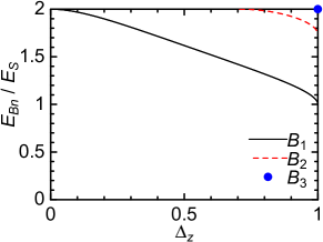
Figure 1: (Color online) Ratio of the $n$-th breather mass $E_{B_{n}}$ to the soliton mass $E_{S}$ as a function of the XXZ anisotropy $\Delta_{z}$ in the sine-Gordon model (9) or (14).

Masses of the soliton, antisoliton and breathers are related to the excitation gaps of the original lattice systems, Eqs. (8) and (13). The soliton and antisoliton correspond to the lowest excitations which change the $z$ component of total spin $S^{z}_{\rm tot}=\sum_{j}S_{j}^{z}$ by $\pm 1$. On the other hand, the lightest breather is regarded as the lowest excitation with $\Delta S^{z}_{\rm tot}=0$. At the $SU(2)$-symmetric AF point $\Delta_{z}=1$, there are three breathers. The soliton, antisoliton and lightest breather are degenerate and form the spin-1 triplet excitations (so-called magnons). The second lightest breather is interpreted as the singlet excitation with $\Delta S_{\rm tot}=0$. In the ferromagnetic regime $\Delta_{z}<0$, where any breather disappears, the lowest soliton-antisoliton scattering state would correspond to the excitation gap in the sector of $\Delta S_{\rm tot}^{z}=0$.

II.3 ${\boldsymbol{J}}$-${\boldsymbol{J}}_{\boldsymbol{2}}$ antiferromagnetic spin chain

In the previous two subsections, we have completely neglected effects of irrelevant perturbations in the low-energy effective theory. However, as already noted, the $\lambda$ term becomes nearly marginal when the anisotropy $\Delta_{z}$ approaches unity. In this case, the $\lambda$ term is expected to affect several physical quantities. Actually, such effects have been studied in both the models (8) [Ref. Orignac04, ] and (13) [Refs. Oshikawa97, ; Affleck99, ].

It is known Haldane82 that a small AF NNN coupling $J_{2}$ decreases the value of $\lambda$ in the $SU(2)$-symmetric AF Heisenberg chain. Okamoto and Nomura Okamoto92 have shown that the marginal interaction vanishes, i.e., $\lambda\to 0$ in the following model:

$${\cal H}^{\rm nnn}=\sum_{j}(J\boldsymbol{S}_{j}\cdot\boldsymbol{S}_{j+1}+J_{2}\boldsymbol{S}_{j}\cdot\boldsymbol{S}_{j+2}),$$ (16)

with $J_{2}=0.2411J$. On the $J_{2}/J$ axis, this model is located at the Kosterlitz-Thouless transition point between the TLL and a spontaneously dimerized phase. From this fact, if we replace ${\cal H}^{\rm XXX}$ with ${\cal H}^{\rm nnn}$ in the $SU(2)$-symmetric models (8) and (13), namely, if we consider the following models:

$$\tilde{\cal H}^{{\rm XXX}\mathchar 45\relax\delta}= {\cal H}^{\rm nnn}+\sum_{j}(-1)^{j}\delta J\boldsymbol{S}_{j}\cdot\boldsymbol{S}_{j+1},$$ (17a)

$$\tilde{\cal H}^{\rm stag}= {\cal H}^{\rm nnn}+\sum_{j}(-1)^{j}h_{\rm s}S_{j}^{z},$$ (17b)

then their effective theories are much closer to a pure sine-Gordon model. In other words, the predictions from the sine-Gordon model, such as Eqs. (11) and (15), become more reliable.

III Coefficients of Dimer and Spin Operators

From the discussions in Sec. II, one can readily find a way of extracting the values of $d_{xy,z}$ and $a_{1}$ in Eqs. (7) and (5) as follows. We first calculate some low-energy levels in $S_{\rm tot}^{z}=\pm 1$ and $S_{\rm tot}^{z}=0$ sectors of the models (8), (13) and (17) by means of numerical diagonalization method. Since all the Hamiltonians (8), (13) and (17) commute with $S^{z}_{\rm tot}=\sum_{j}S_{j}^{z}$, the numerical diagonalization can be performed in the Hilbert subspace with each fixed $S^{z}_{\rm tot}$. In order to extrapolate gaps to the thermodynamic limit with reasonable accuracy, we use appropriate finite-size scaling methods Cardy84 ; Cardy86 ; Cardy86b ; Shanks55 for spin chains under periodic boundary condition (total number of sites $L=8$, 10, $\cdots$, 28, 30). Secondly, the coefficients $d_{xy,z}$ and $a_{1}$ of the spin-$\frac{1}{2}$ XXZ chain and the $J$-$J_{2}$ chain are determined via the comparison between the sine-Gordon gap formula (11) and numerically evaluated spin gaps for various values of $\delta_{xy,z}$ and $h_{\rm s}$. In this procedure, (as already mentioned) the energy difference between the lowest (i.e., ground-state) and the second lowest levels of the $S_{\rm tot}^{z}=0$ sector (gap with $\Delta S_{\rm tot}^{z}=0$) and that between the ground-state level and the lowest level of the $S_{\rm tot}^{z}=\pm 1$ sector (gap with $\Delta S_{\rm tot}^{z}=\pm 1$) are respectively interpreted as the breather (or soliton-antisoliton scattering state) and soliton masses in the sine-Gordon scheme.

III.1 TLL phase and Numerical diagonalization

In this subsection, we focus on the TLL phase of uniform spin-$\frac{1}{2}$ XXZ chains (1) and test the reliability of our numerical diagonalization. The low-energy properties are described by Eq. (2), which is a free boson theory (i.e., CFT with central charge $c=1$) with some irrelevant perturbations. Generally, the finite-size scaling formula for the excitation spectrum in any CFT has been proved Cardy84 ; Cardy86 to be

$$\Delta E_{\cal O}\equiv E_{\cal O}-E_{0}=\frac{2\pi v}{La}[{\cal O}]+\cdots.$$ (18)

Here $E_{0}$ and $E_{\cal O}$ are respectively the ground-state energy and the energy of an excited state generating from a primary field ${\cal O}$ in the given CFT. Remaining quantities $[{\cal O}]$, $v$, and $La$ are the scaling dimension of the operator ${\cal O}$, the excitation velocity and the system length, respectively. In the case of the spin chain (1), the bosonization formula (5) indicates that $E_{e^{\pm i\sqrt{\pi}\theta}}$ and $E_{e^{\pm i\sqrt{4\pi}\phi}}$ correspond to the excitation energies in the $S_{\rm tot}^{z}=\pm 1$ and $S_{\rm tot}^{z}=0$ sectors, respectively. The irrelevant perturbations can also contribute to the finite-size correction to excitation energies. From the $U(1)$ and translational symmetries of the XXZ chain (1), one can show that the finite-size gap $\Delta E_{\Delta S_{\rm tot}^{z}=\pm 1}$ has no significant modification from the perturbations, while the correction to $\Delta E_{\Delta S_{\rm tot}^{z}=0}$ is proportional to $L^{1-[{\rm e}^{{\rm i}2\sqrt{4\pi}\phi}]}$. Therefore, the following finite-size scaling formulas are predicted:

$$\Delta E_{\Delta S_{\rm tot}^{z}=\pm 1}\approx\frac{2\pi v}{La}\frac{1}{4K}+\cdots,$$ (19a)

$$\Delta E_{\Delta S_{\rm tot}^{z}=0}\approx\frac{2\pi v}{La}K+c_{0}L^{1-4K}+\cdots,$$ (19b)

with $c_{0}$ being a non-universal constant. Here we have used $[{\rm e}^{{\rm i}n\sqrt{\pi}\theta}]=n^{2}/(4K)$ and $[{\rm e}^{{\rm i}n\sqrt{4\pi}\phi}]=n^{2}K$. At the $SU(2)$-symmetric AF point $\Delta_{z}=1$, $\Delta E_{\Delta S_{\rm tot}^{z}=\pm 1}=\Delta E_{\Delta S_{\rm tot}^{z}=0}\equiv\Delta E_{\rm su2}$ holds and the marginal $\lambda$ term modifies the scaling form of the spin gap. The marginal term is known to yield a logarithmic correction as follows: Cardy86b

$$\Delta E_{\rm su2}\approx\frac{2\pi v}{La}\left(\frac{1}{2}+\frac{c_{1}}{\ln L}+\frac{c_{2}}{(\ln L)^{2}}+\cdots\right).$$ (20)

Here $c_{1,2}$ are non-universal constants.

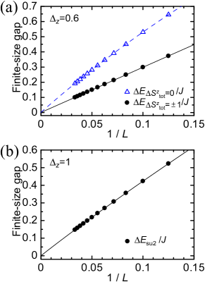
Figure 2: (Color online) (a) Numerically evaluated gaps with $\Delta S^{z}_{\rm tot}=\pm 1$ (circles) and $\Delta S^{z}_{\rm tot}=0$ (triangles) for XXZ chains with $\Delta_{z}=0.6$ and finite length $L$. The solid curve $8.019\times 10^{-4}+2.977/L$ (dashed curve $1.312\times 10^{-3}+5.982/L-4.764/L^{1.8376}$) is determined by fitting the circles (triangles). (b) Gaps of finite-size Heisenberg chains with $\Delta_{z}=1$. The solid curve is $\Delta E_{\rm su2}/J=2.173\times 10^{-4}+4.965/L-2.203/(L\ln L)+1.200/(L(\ln L)^{2})$.

As an example, numerically evaluated gaps with $\Delta S^{z}_{\rm tot}=\pm 1$ and $\Delta S^{z}_{\rm tot}=0$ in the case of $\Delta_{z}=0.6$ are respectively represented as circles and triangles in Fig. 2(a). Circles are nicely fitted by the solid curve $\Delta E_{\Delta S_{\rm tot}^{z}=\pm 1}/J=8.019\times 10^{-4}+2.977/L$. This result is consistent with the fact that an easy-plane anisotropic XXZ model is gapless in the thermodynamic limit and that the exact coefficient of the $1/L$ term is $2\pi v/(4JK)=3$ at $\Delta_{z}=0.6$. Similarly, triangles can be fitted by $\Delta E_{\Delta S_{\rm tot}^{z}=0}/J=1.312\times 10^{-3}+5.982/L-4.764/L^{1.8376}$ where $1.8376=1-4K$. The factor 5.982 of the $1/L$ term is very close to $2\pi vK/(Ja)=6.040$. The spin gap at $SU(2)$-symmetric point is also represented in Fig. 2(b). Following the formula (20), we can correctly determine the fitting curve $\Delta E_{\rm su2}/J=2.173\times 10^{-4}+4.965/L-2.203/(L\ln L)+1.200/(L(\ln L)^{2})$, in which the factor of the second term is nearly equal to $\pi v/(Ja)=4.935$. These results support the reliability of our numerical diagonalization. We note that a more precise finite-size scaling analysis for AF Heisenberg model has been performed in Ref. Nomura93, .

III.2 Dimer coefficients of XY model

Next, let us move onto the evaluation of excitation gaps in dimerized XXZ chains. In this case, since the system is not critical, the above finite-size scaling based on CFT cannot be applied. Instead, we utilize Aitken-Shanks method Shanks55 to extrapolate our numerical data to the values in the thermodynamic limit.

In this subsection, we consider a special dimerized XY chain with $\Delta_{z}=\delta_{z}=0$. It is mapped to a solvable free fermion system through Jordan-Wigner transformation. Therefore, our numerically determined coefficients in Eq. (7) can be compared with the exact value. The lowest energy gap with $\Delta S_{\rm tot}^{z}=\pm 1$, which corresponds to the soliton mass $E_{S}$, is exactly evaluated as

$$\Delta E_{\Delta S_{\rm tot}^{z}=\pm 1}/J=\delta_{xy}.$$ (21)

Comparing Eq. (21) with Eq. (11), we obtain the exact coefficient

$$d_{xy}=1/\pi=0.3183$$ (22)

at the XY case $\Delta_{z}=\delta_{z}=0$. The exact solution also tells us that the excitation gap with $\Delta S_{\rm tot}^{z}=0$ is

$$\Delta E_{\Delta S_{\rm tot}^{z}=0}/J=2\delta_{xy}.$$ (23)

This is consistent with the sine-Gordon prediction that any breather disappears and the relation $E_{B_{1}}=2E_{S}$ holds just at the XY point $\Delta_{z}=0$.

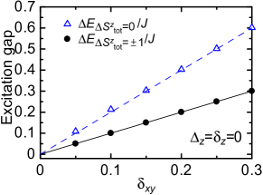
Figure 3: (Color online) Numerically evaluated gaps $\Delta E_{\Delta S_{\rm tot}^{z}=\pm 1}$ (circles) and $\Delta E_{\Delta S_{\rm tot}^{z}=0}$ (triangles) in dimerized XY models with $\Delta_{z}=\delta_{z}=0$. Solid and dashed lines are the exact results determined via Jordan-Wigner transformation. These lines respectively correspond to the soliton and breather masses in the framework of sine-Gordon theory.

Figure 3 shows the comparison between the energy gap calculated by numerical diagonalization with Aitken-Shanks process and Eq. (21) [or Eq. (23)]. Except for $\Delta E_{\Delta S_{\rm tot}^{z}=0}$ in the weak dimerized regime $\delta_{xy}\lesssim 0.1$, numerically calculated gaps coincide well with the exact value. We have found that when $\delta_{xy,z}$ becomes smaller, the precision of Aitken-Shanks method is decreased due to a large size dependence of gaps.

III.3 Dimer coefficients of XXZ model

Table 1: Dimer coefficients ($d_{xy}$ and $d_{z}$), TLL parameter $K$, compactification radius $R$, spinon velocity $v$ of spin-$\frac{1}{2}$ XXZ chain. Dimerization-induced gaps are also listed in the final column. The final line is the result for the $J$-$J_{2}$ chain (16). The same data of $d_{xy,z}$ are also shown in Fig. 4.

$\Delta_{z}$	$d_{xy}$	$d_{z}$	$K$	$R$	$v/(Ja)$	soliton gap $E_{S}/J$
$1$	0.228 (0.204)	0.110 (0.097)	0.5	0.3989($=1/\sqrt{2\pi}$)	1.571($=\pi/2$)	$3.535(\delta_{xy}d_{xy}+\delta_{z}d_{z})^{0.6667}$
$0.9$	0.278 (0.261)	0.141 (0.131)	0.5838	0.3692	1.518	$3.268(\delta_{xy}d_{xy}+\delta_{z}d_{z})^{0.7061}$
$0.8$	0.297 (0.284)	0.154 (0.146)	0.6288	0.3557	1.465	$3.147(\delta_{xy}d_{xy}+\delta_{z}d_{z})^{0.7293}$
$0.7$	0.309 (0.299)	0.165 (0.159)	0.6695	0.3448	1.410	$3.057(\delta_{xy}d_{xy}+\delta_{z}d_{z})^{0.7516}$
$0.6$	0.318 (0.310)	0.174 (0.169)	0.7094	0.3349	1.355	$2.986(\delta_{xy}d_{xy}+\delta_{z}d_{z})^{0.7748}$
$0.5$	0.324 (0.318)	0.182 (0.177)	0.75	0.3257	1.299	$2.934(\delta_{xy}d_{xy}+\delta_{z}d_{z})^{0.8}$
$0.4$	0.327 (0.323)	0.188 (0.185)	0.7924	0.3169	1.242	$2.902(\delta_{xy}d_{xy}+\delta_{z}d_{z})^{0.8281}$
$0.3$	0.328 (0.325)	0.193 (0.191)	0.8375	0.3082	1.184	$2.893(\delta_{xy}d_{xy}+\delta_{z}d_{z})^{0.8602}$
$0.2$	0.328 (0.325)	0.197 (0.196)	0.8864	0.2996	1.124	$2.918(\delta_{xy}d_{xy}+\delta_{z}d_{z})^{0.8980}$
$0.1$	0.324 (0.323)	0.200 (0.200)	0.9401	0.2910	1.063	$2.991(\delta_{xy}d_{xy}+\delta_{z}d_{z})^{0.9434}$
$0$	0.318 (0.318)	0.202 (0.203)	1	0.2821($=1/\sqrt{4\pi}$)	1	$3.141(\delta_{xy}d_{xy}+\delta_{z}d_{z})$
$-0.1$	0.309 (0.311)	0.202 (0.204)	1.068	0.2730	0.9353	$3.431(\delta_{xy}d_{xy}+\delta_{z}d_{z})^{1.073}$
$-0.2$	0.297 (0.302)	0.200 (0.204)	1.147	0.2634	0.8685	$4.008(\delta_{xy}d_{xy}+\delta_{z}d_{z})^{1.172}$
$-0.3$	0.278 (0.289)	0.194 (0.203)	1.241	0.2533	0.7990	$5.308(\delta_{xy}d_{xy}+\delta_{z}d_{z})^{1.317}$
$-0.4$	0.252 (0.273)	0.184 (0.199)	1.355	0.2423	0.7263	$9.214(\delta_{xy}d_{xy}+\delta_{z}d_{z})^{1.550}$
$-0.5$	0.213 (0.248)	0.163 (0.191)	1.5	0.2303	0.6495	$33.25(\delta_{xy}d_{xy}+\delta_{z}d_{z})^{2}$
$J$-$J_{2}$ model	0.364 (0.361)	0.188 (0.182)	0.5	0.3989	1.174	$3.208(\delta_{xy}d_{xy}+\delta_{z}d_{z})^{0.6667}$

In the easy-plane region $-1<\Delta_{z}<1$, any generic analytical way of determining the coefficients in Eq. (7) has never been known except for the above special point $\Delta_{z}=\delta_{z}=0$. To obtain $d_{xy}$ (respectively $d_{z}$), we numerically calculate excitation gaps at the points $\delta_{xy}$ $(\delta_{z})=0.05$, 0.1, $\cdots$, 0.3 with fixing $\delta_{z}(\delta_{xy})=0$. Although both $\Delta E_{\Delta S_{\rm tot}^{z}=0}$ and $\Delta E_{\Delta S_{\rm tot}^{z}=\pm 1}$ are applicable to determine $d_{xy,z}$ in principle, we use only the latter gap since it more smoothly converges to its thermodynamic-limit value via Aitken-Shanks process, compared to the former. In fact, Eq. (19) suggests that $\Delta E_{\Delta S_{\rm tot}^{z}=0}$ is subject to effects of irrelevant perturbations and therefore contains complicated finite-size corrections. Coefficients $d_{xy}$ ($d_{z}$) can be determined for each $\delta_{xy}$ ($\delta_{z}$) from Eq. (11). Since the field theory result (11) is generally more reliable as the perturbation $\delta_{xy,z}$ is smaller, we should compare Eq. (11) with excitation gaps determined at sufficiently small values of $\delta_{xy,z}$. However, the extrapolation to thermodynamic limit by Aitken-Shanks method is less precise in such a small dimerization region mainly due to large finite-size effects. Papenbrock03 ; Orignac04 Therefore, we adopt coefficients $d_{xy,z}$ extracted from the gaps at relatively large dimerization $\delta_{xy(z)}=0.1$ and $0.3$, and they are listed in Table 1: the values outside [inside] parentheses are the data for $\delta_{xy(z)}=0.3$ [0.1]. The anisotropy dependence of the same data $d_{xy,z}$ is depicted in Fig. 4. The data in Table 1 and Fig. 4 are the main result of this paper. The difference between $d_{xy(z)}$ outside and inside the parentheses in Table 1 could be interpreted as the ”strength” of irrelevant perturbations neglected in the effective sine-Gordon theory or the ”error” of our numerical strategy. The neglected operators must bring a renormalization of coefficients $d_{xy,z}$, and the ”error” would become larger as the system approaches the Heisenberg point since (as already mentioned) the $\lambda$ term becomes marginal at the point.

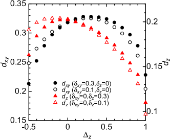
Figure 4: (Color online) XXZ-anisotropy ($\Delta_{z}$) dependence of dimer coefficients $d_{xy}$ and $d_{z}$. Filled [Open] circles represent $d_{xy}$ determined from dimerization gap at $(\delta_{xy},\delta_{z})=(0.3,0)$ [$=(0.1,0)$]. Similarly, filled [open] triangles show $d_{z}$ determined from dimerization gap at $(\delta_{xy},\delta_{z})=(0,0.3)$ [$=(0,0.1)$].

We here discuss the validity of the numerically determined $d_{xy,z}$ in Table 1 and Fig. 4. Table 1 shows that in the wide range $-0.3\lesssim\Delta_{z}\lesssim 0.9$, the difference (error) between $d_{xy,z}$ outside and inside the parentheses is less than 8 $\%$. As expected, one finds that the error gradually increases when the anisotropy $\Delta_{z}$ approaches unity. Similarly, the error is large in the deeply ferromagnetic regime $\Delta_{z}\lesssim-0.3$. This is naturally understood from the fact that as $\Delta_{z}$ is negatively increased, the dimerization term $\sin(\sqrt{4\pi}\phi)$ becomes less relevant and effects of other irrelevant terms is relatively strong. Indeed, for $\Delta_{z}<-0.7071$ ($K>2$), the dimerization does not yield any spin gap and our method of determining $d_{xy,z}$ cannot be used. Furthermore, it is worth noting that the spin gap is convex downward as a function of dimerization $\delta_{xy,z}$ in the ferromagnetic side $\Delta_{z}<0$, and the accuracy of the fitting therefore depreciates.

In addition to coefficients $d_{xy,z}$, let us examine dimerization gaps and the quality of fitting by Eq. (11). Excitation gaps for $\Delta_{z}=0.6$ are shown in Fig. 5 as an example. Remarkably, both soliton-gap curves (11) with the values $d_{xy,z}$ outside and inside the parentheses in Table 1 fit the numerical data $\Delta E_{\Delta S_{\rm tot}^{z}=\pm 1}$ in the broad region $0\leq\delta_{xy(z)}\leq 0.3$ with reasonable accuracy. The former solid curve is slightly better that the latter. The breather gaps $\Delta E_{\Delta S_{\rm tot}^{z}=0}$ and corresponding fitting curves are also shown in Fig. 5. This breather curve is determined by combining the solid curve (11) and the soliton-breather relation (10). It slightly deviates from numerical data, especially, in a relatively large dimerization regime $0.15\lesssim\delta_{xy(z)}$. As mentioned above, this deviation would be attributed to irrelevant perturbations. The breather-soliton mass ratio $E_{B_{1}}/E_{S}$ [see Eq. (10)] in the sine-Gordon model (9) and the numerically evaluated $\Delta E_{\Delta S_{\rm tot}^{z}=0}/\Delta E_{\Delta S_{\rm tot}^{z}=\pm 1}$ are shown in Fig. 6. These two values are in good agreement with each other in the wide parameter region $-0.5<\Delta_{z}<1$, although their difference becomes slightly larger in the region $0.5\lesssim\Delta_{z}\lesssim 1$, which includes the point $\Delta_{z}=0.6$ in Fig. 5. Gaps $\Delta E_{\Delta S_{\rm tot}^{z}=\pm 1}$ for dimerized XXZ chains with several values of both $\delta_{xy}$ and $\delta_{z}$ are plotted in Fig. 7. It shows that the numerical data are quantitatively fitted by the single gap formula (11). All of the results in Figs. 5-7 indicates that a simple sine-Gordon model (9) can describe the low-energy physics of the dimerized spin chain (8) with reasonable accuracy in the wide easy-plane regime. This also supports the validity of our numerical approach for fixing the coefficients $d_{xy,z}$.

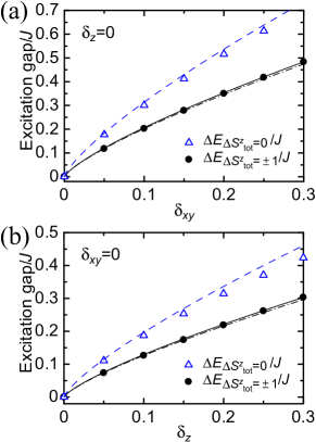
Figure 5: (Color online) Excitation gaps $\Delta E_{\Delta S_{\rm tot}^{z}=\pm 1}$ (circles) and $\Delta E_{\Delta S_{\rm tot}^{z}=0}$ (triangles) of the dimerized XXZ model (8) with $\Delta_{z}=0.6$. Solid and dashed-dotted curves are fitted by the gap formula (11) with coefficients outside and inside parentheses in Table 1, respectively. The dashed curve represents the lightest breather mass which is fixed by combining the solid soliton curve and Eq. (10).

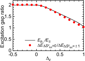
Figure 6: (Color online) Ratio between two numerically evaluated gaps $\Delta E_{\Delta S_{\rm tot}^{z}=0}/\Delta E_{\Delta S_{\rm tot}^{z}=\pm 1}$ (circles) in the dimerized chain (8) with $\delta_{xy}=0.3$ and $\delta_{z}=0$. Solid curve is the soliton-breather mass ratio $E_{B_{1}}/E_{S}$ in the effective sine-Gordon theory (9). Note that in the ferromagnetic side $\Delta_{z}<0$, there is no breather and $E_{B_{1}}$ is replaced with the mass gap of soliton-antisoliton scattering states $2E_{S}$, namely, $E_{B_{1}}/E_{S}\to 2E_{S}/E_{S}=2$.

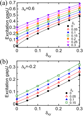
Figure 7: (Color online) Numerically evaluated gaps $\Delta E_{\Delta S_{\rm tot}^{z}=\pm 1}$ of dimerized XXZ chains with several values of both parameters $\delta_{xy}$ and $\delta_{z}$ at $\Delta_{z}=0.6$ and $-0.2$. Solid curves are Eq. (11) with $d_{xy}$ and $d_{z}$ in Table 1. In the ferromagnetic case $\Delta_{z}=-0.2$, the analytical curve successfully fits the numerical data for a wide weakly-dimerized regime $\delta_{xy,z}\ll 1$, while the deviation occurs for the strongly-dimerized one.

III.4 Dimer coefficients of SU(2)-symmetric models

At the $SU(2)$-symmetric AF point, the $\lambda$ term in the effective Hamiltonian (2) becomes marginal and induces logarithmic corrections to several physical quantities. Such a logarithmic fashion often makes the accuracy of numerical methods decrease. Instead of numerical approaches, using the asymptotic form of the spin correlation function Affleck98 and OPE technique, Gogolin ; Tsvelik Orignac Orignac04 has predicted

$$d_{xy}=2d_{z}=\frac{2}{\pi^{2}}\left(\frac{\pi}{2}\right)^{1/4}=0.2269$$ (24)

at the $SU(2)$-symmetric point. Substituting Eq. (24) into Eq. (11), the spin gap in a $SU(2)$-symmetric AF chain with dimerization $\delta_{xy}=\delta_{z}\equiv\delta$ (${\cal H}^{{\rm XXX}\mathchar 45\relax\delta}$) is determined as

$$\Delta E_{\rm su2}/J=1.723\delta^{2/3}.$$ (25)

The marginal term however produces a correction to this result. It has been shown in Ref. Orignac04, that the spin gap in the model ${\cal H}^{{\rm XXX}\mathchar 45\relax\delta}$ is more nicely fitted with

$$\Delta E_{\rm su2}/J=\frac{1.723\delta^{2/3}}{\left(1+0.147\ln\Big{|}\frac{0.1616}{\delta}\Big{|}\right)^{1/2}},$$ (26)

from the renormalization-group argument. As can be seen from Eq. (26), the logarithmic correction is not significantly large for the spin gap. We may therefore apply the way based on the sine-Gordon model in Sec. III.3 even for the present AF Heisenberg model. The resultant data are listed in the first line of Table 1. Evaluated coefficients $d_{xy}=0.228$ (0.204) and $d_{z}=0.110$ (0.097) are fairly close to the results of Eq. (24). This suggests that the effect of the marginal operator on the spin gap is really small. We should also note that $d_{xy}=2d_{z}$ is approximately realized, which is required from the $SU(2)$ symmetry. The numerically calculated spin gap $\Delta E_{\rm su2}$, Eq. (26), and the curve of the gap formula (11) are shown in Fig. 8(a). It is found that even the curve without any logarithmic correction can fit the numerical data within semi-quantitative level. At least, parameters $d_{xy,z}$ at the $SU(2)$-symmetric point can be regarded as effective coupling constants when we naively approximate a dimerized Heisenberg chain as a simple sine-Gordon model.

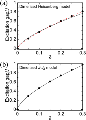
Figure 8: (Color online) Spin gaps (circles) of (a) the Heisenberg model with dimerization $\delta_{xy}=\delta_{z}=\delta$ and (b) the dimerized $J$-$J_{2}$ model (17a). Both solid curves in panels (a) and (b) are determined from the gap formula (11). The dashed curve in panel (a) represents Eq. (26).

As discussed in Sec. II.3, logarithmic corrections vanish in the $J$-$J_{2}$ model (16) due to the absence of the marginal operator. As expected, Fig. 8(b) shows that the spin gap $\Delta E_{\rm su2}$ is accurately fitted by the sine-Gordon gap formula (11) in the wide range $0\leq\delta\leq 0.3$. Therefore, the coefficients $d_{xy,z}$ of the $J$-$J_{2}$ model (the final line of Table 1) are highly reliable. Remarkably, the difference between the values outside and inside the parentheses is much smaller than that of the Heisenberg model (the first and last line of Table 1). Here, to determine $d_{xy,z}$ of the $J$-$J_{2}$ model, we have used its spinon velocity $v=1.174Ja$, which has been evaluated in Ref. Okamoto97, .

III.5 Coefficients of spin operator

In this subsection, we discuss the spin-operator coefficient $a_{1}$ in Eq. (5). Although $a_{1}$ for the easy-plane XXZ model has been evaluated analytically Lukyanov97 ; Lukyanov99 ; Lukyanov03 and numerically, Hikihara98 ; Hikihara04 those for the $SU(2)$-symmetric Heisenberg chain and the $J$-$J_{2}$ model have never been studied. The existent data also help us to check the validity of our method. From the bosonization formula (5), the $z$-component spin correlation function has the following asymptotic form:

$$\langle S_{j}^{z}S_{j^{\prime}}^{z}\rangle=-\frac{1}{4\pi^{2}\eta|j-j^{\prime}|^{2}}+\frac{A_{1}^{z}(-1)^{j-j^{\prime}}}{|j-j^{\prime}|^{1/\eta}}+\cdots,$$ (27)

in the easy-plane TLL phase. The amplitude $A_{1}^{z}$ is related to $a_{1}$ as

$$A_{1}^{z}=a_{1}^{2}/2.$$ (28)

Lukyanov and his collaborators Lukyanov97 ; Lukyanov99 have predicted

$$A_{1}^{z}=\frac{2}{\pi^{2}}\left[\frac{\Gamma(\frac{\eta}{2-2\eta})}{2\sqrt{\pi}\Gamma(\frac{1}{2-2\eta})}\right]^{1/\eta}$$

$$\times\exp\left[\int_{0}^{\infty}\frac{{\rm d}t}{t}\left(\frac{\sinh[(2\eta-1)t]}{\sinh(\eta t)\cosh[(1-\eta)t]}-\frac{2\eta-1}{\eta}{\rm e}^{-2t}\right)\right].$$ (29)

The same amplitude has been calculated by using DMRG in Refs. Hikihara98, ; Hikihara04, .

Table 2: Spin-operator coefficients $a_{1}$ of spin-$\frac{1}{2}$ XXZ chain and the $J$-$J_{2}$ chain. Values in column (A), (B), and (C) correspond to the analytical prediction from Refs. Lukyanov97, ; Lukyanov99, ; Lukyanov03, , the result by DMRG in Refs. Hikihara98, ; Hikihara04, , and ours, respectively.

$\Delta_{z}$	$a_{1}$ (A)	$a_{1}$ (B)	$a_{1}$ (C)	$\eta$	$v/(Ja)$	soliton gap $E_{S}/J$
1			0.4724 (0.4325)	1	1.571	$3.535(a_{1}h_{\rm s}/J)^{0.6667}$
0.9	0.7049	0.64	0.5327 (0.4830)	0.8564	1.518	$3.268(a_{1}h_{\rm s}/J)^{0.7061}$
0.8	0.6069	0.587	0.5226 (0.4808)	0.7952	1.465	$3.147(a_{1}h_{\rm s}/J)^{0.7293}$
0.7	0.5464	0.54	0.5019 (0.4693)	0.7468	1.410	$3.057(a_{1}h_{\rm s}/J)^{0.7516}$
0.6	0.5008	0.499	0.4771 (0.4530)	0.7048	1.355	$2.986(a_{1}h_{\rm s}/J)^{0.7748}$
0.5	0.4629	0.4626	0.4505 (0.4338)	0.6667	1.299	$2.934(a_{1}h_{\rm s}/J)^{0.8}$
0.4	0.4297	0.4297	0.4235 (0.4127)	0.6310	1.242	$2.902(a_{1}h_{\rm s}/J)^{0.8281}$
0.3	0.3994	0.3995	0.3966 (0.3903)	0.5970	1.184	$2.893(a_{1}h_{\rm s}/J)^{0.8602}$
0.2	0.3712	0.3713	0.3701 (0.3670)	0.5641	1.124	$2.918(a_{1}h_{\rm s}/J)^{0.8980}$
0.1	0.3443	0.3443	0.3440 (0.3430)	0.5319	1.063	$2.991(a_{1}h_{\rm s}/J)^{0.9434}$
0	0.3183	0.3183	0.3183 (0.3183)	0.5	1	$3.141(a_{1}h_{\rm s}/J)$
$J$-$J_{2}$ model			0.4693 (0.4668)	1	1.174	$3.208(a_{1}h_{\rm s}/J)^{0.6667}$

In order to determine $a_{1}$, we use XXZ models in a staggered field (13). Following the similar way to Sec. III.3, we can extract the coefficient $a_{1}$ by fitting numerically evaluated gaps of the model (13) through the sine-Gordon gap formula (15). We numerically estimate the gaps at $h_{\rm s}/J=0.01$, 0.02, $\cdots$, 0.09, 0.1, 0.2, and 0.3 via Aitken-Shanks method. The results are listed in column (C) of Table 2. Similarly to the case of dimerization, we adopt spin gaps at relatively large staggered fields $h_{s}/J=0.1$ and $0.3$ to determine the coefficients $a_{1}$. The value outside (inside) the parentheses in Table 2 corresponds to $a_{1}$ fixed at $h_{\rm s}/J=0.1$ (0.3). Note that the XY model in a staggered field is solvable through Jordan-Wigner transformation, and as a result the coefficient $a_{1}$ is exactly evaluated as

$$a_{1}=1/\pi=0.3183.$$ (30)

The table clearly shows that the values at $h_{\rm s}/J=0.1$ are closer to those of the previous prediction in Refs. Lukyanov97, ; Lukyanov99, ; Lukyanov03, ; Hikihara98, ; Hikihara04, . We emphasize that our results gradually deviate from the analytical prediction from Eq. (29) as the system approaches the $SU(2)$-symmetric point. The same property also appears in the DMRG results in Refs. Hikihara98, ; Hikihara04, . Actually, $A_{1}^{z}$ in Eq. (29) diverges when $\Delta_{z}\to 1$. However, the bosonization formula (5) for spin operators must be still used even around $\Delta_{z}=1$. Thus we should realize that the relation (28) is broken and $a_{1}$ remains to be finite at the $SU(2)$-symmetric point. Figure 9 represents the numerically evaluated gaps $\Delta E_{\Delta S_{\rm tot}^{z}=\pm 1}$, and three fitting curves fixed by $a_{1}$ (A) and $a_{1}$ (C) outside and inside the parentheses in Table 2. Our coefficient $a_{1}$ successfully fits the numerical data semi-quantitatively in the wide regime $0.01\lesssim h_{\rm s}/J\lesssim 0.3$, while the curve of $a_{1}$ (A) is valid only in an extremely weak staggered-field regime $0<h_{\rm s}/J\lesssim 0.01$. This implies that when $\Delta_{z}$ is near unity, the field theory description based on Eqs. (28) and (29) is valid only in a quite narrower region for the present staggered-field case compared to the case of dimerized spin chain. On the other hand, Fig. 9 also suggests that if we use $a_{1}$ (C) in Table 2 as the effective coefficient of bosonized spin operator instead of $a_{1}$ (A) and (B), the XXZ chain in a staggered field (13) may be approximated by a simple sine-Gordon model in wide region $0.01\lesssim h_{\rm s}/J\lesssim 0.3$.

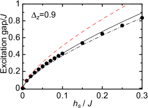
Figure 9: (Color online) Spin gaps $\Delta E_{\Delta S_{\rm tot}^{z}=\pm 1}$ (circles) of the XXZ models in a staggered field at $\Delta_{z}=0.9$. Solid and dashed-dotted curves are determined from the gap formula (15) with $a_{1}$ outside and inside the parentheses in Table 2, respectively. The dashed curve is given by the formula (15) with $a_{1}$ in Refs. Lukyanov97, ; Lukyanov99, ; Lukyanov03, [i.e., $a_{1}$ determined from Eq. (29)].

At the $SU(2)$-symmetric point $\Delta_{z}=1$, a logarithmic correction to staggered-field induced gaps is expected to appear due to the marginal perturbation. This makes it difficult to extract the value $a_{1}$ within the present sine-Gordon framework. According to the prediction in Ref. Orignac04, based on the asymptotic form of spin correlation function, Affleck98 $a_{1}$ is given by

$$a_{1}=\frac{1}{\pi}\Big{(}\frac{\pi}{2}\Big{)}^{1/4}=0.3564$$ (31)

at the $SU(2)$-symmetric point, where $a_{1}=b_{0}$ is imposed. The spin gap in AF Heisenberg chains in a staggered field (${\cal H}^{{\rm stag}}$ with $\Delta_{z}=1$) is thus determined as

$$\Delta E_{\Delta S_{\rm tot}^{z}=\pm 1}/J=1.777(h_{\rm s}/J)^{2/3}.$$ (32)

A more correct gap formula including the logarithmic correction has been developed in Refs. Oshikawa97, ; Affleck99, as follows:

$$\Delta E_{\Delta S_{\rm tot}^{z}=\pm 1}/J=1.85(h_{\rm s}/J)^{2/3}[\ln(J/h_{\rm s})]^{1/6}.$$ (33)

In Fig. 10(a), the numerically evaluated spin gaps, Eq. (33), and the fitting curve with $a_{1}$ outside the parentheses in column (C) are drawn. One finds that both curves agree well with the numerical data in the weak-field regime $0<h_{\rm s}/J\lesssim 0.1$, while they start to deviate from the data in the stronger-field regime. This suggests that even at the $SU(2)$-symmetric point, a simple sine-Gordon description for the model (13) is applicable in the relatively wide region $0<h_{\rm s}/J\lesssim 0.1$, if the coefficient $a_{1}$ outside the parentheses in column (C) is adopted.

In the same way as the final paragraph in Sec. III.4, we can accurately determine the coefficient $a_{1}=b_{0}$ for the $J$-$J_{2}$ model since the marginal perturbation vanishes. The data are listed in the final line in Table 2. One sees from Fig. 10(b) that the spin gap $\Delta E_{\Delta S_{\rm tot}^{z}=\pm 1}$ is fitted by the gap formula (15) quite accurately. In addition, the difference between the values outside and inside the parentheses is significantly small.

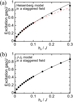
Figure 10: (Color online) Spin gaps $\Delta E_{\Delta S_{\rm tot}^{z}=\pm 1}$ (circles) of (a) the Heisenberg and (b) the $J$-$J_{2}$ models (17b) in a staggered field. Solid and dashed curves represent Eq. (15) and Eq. (33), respectively. We have used $a_{1}$ outside the parentheses in column (C) of Table 2.

III.6 Coefficients determined from ground-state energy

Instead of the gap formula (11), the formula for ground-state energy (12) can also be utilized to determine dimer coefficients $d_{xy,z}$. Let us here define $\Delta E_{\rm GS}\equiv E_{\rm GS}-E_{\rm GS}(\delta_{xy},\delta_{z})$, where $E_{\rm GS}$ is the ground-state energy of the XXZ chain (1) per site and $E_{\rm GS}(\delta_{xy},\delta_{z})$ is that of the bond-alternating XXZ chain (8). If the dimerization parameter is small enough $|\delta_{xy,z}|\ll 1$, $\Delta E_{\rm GS}$ is expected to agree well with $\Delta{\cal E}_{\rm GS}$ in Eq. (12). In this case, we can extract the values of $d_{xy,z}$ from the relation $\Delta E_{\rm GS}=\Delta{\cal E}_{\rm GS}$.

To extrapolate the thermodynamic-limit value of $E_{\rm GS}(\delta_{xy},\delta_{z})$, we use Aitken-Shanks method for the results of finite-size numerical diagonalization, and the method works well since the bond-alternating chains are gapful. On the other hand, $E_{\rm GS}$ includes a large finite-size correction, as shown in Sec. III.1. Therefore, instead of numerically-evaluated $E_{\rm GS}$, we use its exact value fixed by Bethe ansatz Yang66

$$\frac{E_{\rm GS}}{J}= \frac{1}{4}\cos\gamma-\frac{1}{2}\sin^{2}\gamma$$

$$\;\times\int_{-\infty}^{\infty}\frac{{\rm d}\lambda}{\cosh(\pi\lambda)}\frac{1}{\cosh(2\gamma\lambda)-\cos\gamma},$$ (34)

where $\gamma\equiv\cos^{-1}\Delta_{z}$. At the limit of $\gamma\to 0$, we obtain the ground-state energy for the Heisenberg model,

$$\left.\frac{E_{\rm GS}}{J}\right|_{\gamma\to 0}=\frac{1}{4}-\ln 2.$$ (35)

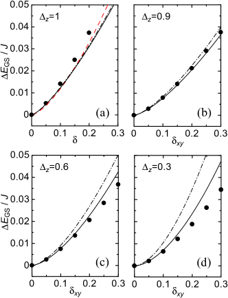
Figure 11: (Color online) (a) Ground-state energy difference $\Delta E_{\rm GS}$ for the $SU(2)$-symmetric case with $\Delta_{z}=1$ and $\delta_{xy}=\delta_{z}=\delta$, obtained from numerical diagonalization (black circles). Solid and dashed-dotted curves represent Eq. (12) with $d_{xy[z]}$ determined from the relation $\Delta{\cal E}_{\rm GS}=\Delta E_{\rm GS}$ at $(\delta_{xy},\delta_{z})=(0.05,0)$ [$=(0,0.05)$] and with those in Table 1, respectively. Dashed curve is Eq. (36) including the logarithmic correction. In the panels (b), (c), and (d), black circles are $\Delta E_{\rm GS}$ for $\Delta_{z}=0.9$, $0.6$, and $0.3$, respectively, under the condition $\delta_{z}=0$. Solid and dashed-dotted curves are respectively Eq. (12) with $d_{xy}$ obtained through $\Delta{\cal E}_{\rm GS}=\Delta E_{\rm GS}$ at $\delta_{xy}=0.05$ and with that in Table 1.

Black points in Fig. 11 show $\Delta E_{\rm GS}$ determined from Eq. (34) and numerically evaluated $E_{\rm GS}(\delta_{xy},\delta_{z})$ for the cases of $\Delta_{z}=1$, 0.9, 0.6 and $0.3$. The solid curve in the panel (a) of this figure represents the formula (12) with $d_{xy[z]}$ determined from $\Delta E_{\rm GS}$ at $(\delta_{xy},\delta_{z})=(0.05,0)[=(0,0.05)]$. Solid curves in the panels (b), (c), (d) are also the formula (12) with $d_{xy}$ obtained in the same way. For comparison, we also draw dashed-dotted curves of the formula (12) with the coefficients in Table 1. In the $SU(2)$ case of the panel (a), the ground-state energy formula with a logarithmic correction

$$\frac{\Delta E_{\rm GS}}{J}=\frac{0.2728\delta^{4/3}}{1+0.147\ln\left|\frac{0.1616}{\delta}\right|},$$ (36)

which is predicted in Ref. Orignac04, , is also plotted as a dashed curve. As pointed out in Ref. Orignac04, , we find that even the curve including the correction deviates from the numerical data for $\delta\gtrsim 0.1$. On top of this isotropic case, Fig. 11 shows that the accuracy of the fitting curves becomes worse as the anisotropy $\Delta_{z}$ decreases. This is a natural result from the fact that the formula (12) is broken down at the XY point with $\Delta_{z}=0$ and $\eta=1/2$. The deviation between the numerical data and the curve also becomes larger for $\delta\gtrsim 0.1$ in the easy-plane region except for the case around $\Delta_{z}=0.9$. This sharply contrasts with the firm correspondence between dimerization gap and the sine-Gordon gap formula (11) (see, e.g, Figs. 3-8). We therefore determine the coefficients $d_{xy[z]}$ by using the numerical data $\Delta E_{\rm GS}$ for small dimerization parameters $(\delta_{xy},\delta_{z})=(0.05,0)[=(0,0.05)]$ or $(\delta_{xy},\delta_{z})=(0.1,0)[=(0,0.1)]$. They are summarized in Table 3. There exists a large difference between $d_{xy,z}$ in Tables 1 and 3, especially, in strongly easy-plane region.

In the remaining part of this subsection, we discuss the reason why $\Delta E_{\rm GS}$ fairly deviate from the analytic prediction $\Delta{\cal E}_{\rm GS}$ in contrast to the case of the dimerization gap in Secs. III.2- III.4. Firstly, the sine-Gordon theory is just a perturbative low-energy effective theory for dimerized spin chains, while $\Delta E_{\rm GS}$ would be subject to high-energy states as well as low-energy ones. Therefore, it is expected that the formula (12) can be applicable only in an extremely weak dimerization regime. In fact, we find from Fig. 11 that solid and dashed-dotted curves seem to become close to each other in an extremely weak dimerization regime $\delta_{xy},\delta\lesssim 0.05$. Hence, we conclude that it is dangerous to apply the sine-Gordon formula of the ground-state energy to the original spin chains with moderate dimerization. Secondly, the ground-state energy difference $\Delta E_{\rm GS}$ is always a convex-downward function of $\delta_{xy,z}$ in the whole region $0<\Delta_{z}\leq 1$. This convex property generally makes the accuracy of fitting decrease as the case of the dimerization gap in the ferromagnetic region $\Delta_{z}<0$. Moreover, as mentioned above, the formula (12) becomes invalid in the vicinity of both $\Delta_{z}=1$ and $\Delta_{z}=0$. From these arguments, coefficients $d_{xy,z}$ and $a_{1}$ obtained from low-lying excitation gaps are more reliable.

Table 3: Dimer coefficients $d_{xy,z}$ of spin-$\frac{1}{2}$ XXZ chain obtained from ground-state energy difference $\Delta E_{\rm GS}$. The data outside (inside) the parentheses are fixed by the energy at $\delta_{xy,z}=0.05$ (0.1). The final line is the result for the $J$-$J_{2}$ model.

$\Delta_{z}$	$d_{xy}$	$d_{z}$	$E_{\rm GS}-E_{\rm GS}(\delta_{xy},\delta_{z})$
$1$	0.226 (0.239)	0.107 (0.113)	$1.148(\delta_{xy}d_{xy}+\delta_{z}d_{z})^{1.333}$
$0.9$	0.261 (0.265)	0.131 (0.134)	$1.331(\delta_{xy}d_{xy}+\delta_{z}d_{z})^{1.412}$
$0.8$	0.275 (0.274)	0.143 (0.144)	$1.484(\delta_{xy}d_{xy}+\delta_{z}d_{z})^{1.459}$
$0.7$	0.283 (0.278)	0.152 (0.151)	$1.673(\delta_{xy}d_{xy}+\delta_{z}d_{z})^{1.503}$
$0.6$	0.285 (0.278)	0.159 (0.156)	$1.924(\delta_{xy}d_{xy}+\delta_{z}d_{z})^{1.550}$
$0.5$	0.284 (0.273)	0.162 (0.158)	$2.280(\delta_{xy}d_{xy}+\delta_{z}d_{z})^{1.6}$
$0.4$	0.276 (0.264)	0.163 (0.157)	$2.827(\delta_{xy}d_{xy}+\delta_{z}d_{z})^{1.656}$
$0.3$	0.262 (0.248)	0.159 (0.132)	$3.766(\delta_{xy}d_{xy}+\delta_{z}d_{z})^{1.720}$
$0.2$	0.236 (0.221)	0.149 (0.140)	$5.705(\delta_{xy}d_{xy}+\delta_{z}d_{z})^{1.796}$
$0.1$	0.188 (0.174)	0.123 (0.114)	$11.72(\delta_{xy}d_{xy}+\delta_{z}d_{z})^{1.887}$
$0$	$-$	$-$	$-$
$J$-$J_{2}$	0.342 (0.334)	0.173 (0.171)	$1.265(\delta_{xy}d_{xy}+\delta_{z}d_{z})^{1.333}$

IV Applications

In this section, we apply the results of Sec. III to some magnetic systems. We demonstrate that several physical quantities related to spins or dimerizations can be calculated accurately from the data in Tables 1 and 2.

IV.1 Dimerized spin chains in a uniform field

We first consider a spin-$\frac{1}{2}$ dimerized XXZ chain in a magnetic field. The Hamiltonian is defined as

$${\cal H}^{\delta\mathchar 45\relax H}={\cal H}^{{\rm XXZ}\mathchar 45\relax\delta}-H\sum_{j}S_{j}^{z},$$ (37)

with $\delta_{xy}=\delta$ and $\delta_{z}=\Delta_{z}\delta$. As we have already explained, a spin gap opens in the zero-field case. However, a magnetic field $H>0$ induces the Zeeman splitting, and the gap of the magnon excitation with $S^{z}=1$ ($-1$) decreases (increases) as $\Delta E_{\Delta S_{\rm tot}^{z}=\pm 1}\mp H$. When $H$ becomes larger than the value of the zero-field spin gap, the $S^{z}=1$ magnon condensation takes place and a field-induced TLL phase emerges with an incommensurate Fermi wave number $k_{F}=\pi-2\pi\langle S_{j}^{z}\rangle$. Therefore, the curve of the spin gap as a function of dimerization $\delta$ is directly interpreted as the ground-state phase boundary of the model (37), if the vertical axis (spin gap) is replaced with the strength of the magnetic field $H$. It is shown in Fig. 12.

The critical point between the dimerized and TLL phases can be determined from experiments with varying $H$. Comparing the experimentally obtained critical field $H_{c}$ and the phase diagram of Fig. 12 in quasi 1D dimerized spin-$\frac{1}{2}$ compounds, one can evaluate the strength of the dimerization $\delta$.

Figure 12: (Color online) Ground-state phase diagram of the dimerized spin chains under a magnetic field $H$, Eq. (37). Each curve represents the phase boundary between the dimer and field-induced TLL phases.

IV.2 Two-leg spin ladder with a four-spin interaction

We next consider an $SU(2)$-symmetric two-leg spin-$\frac{1}{2}$ AF ladder with a four-spin exchange, whose Hamiltonian is given by

$${\cal H}^{\rm lad}= \sum_{j}\sum_{r=1,2}J\boldsymbol{S}_{r,j}\cdot\boldsymbol{S}_{r,j+1}+\sum_{j}J_{\perp}\boldsymbol{S}_{1,j}\cdot\boldsymbol{S}_{2,j}$$

$$+\sum_{j}J_{4}(\boldsymbol{S}_{1,j}\cdot\boldsymbol{S}_{1,j+1})(\boldsymbol{S}_{2,j}\cdot\boldsymbol{S}_{2,j+1}).$$ (38)

The symbol $r$ denotes the chain index. Three quantities $J>0$, $J_{\perp}$ and $J_{4}$ respectively stand for the intrachain-, interchain- and four-spin coupling constants. There are at least two kinds of physical origin of the four-spin term $J_{4}$. The first is that optical phonon modes with a spin-Peierls type coupling can cause a negative $J_{4}$. Nersesyan97 The second is that the higher-order expansion of hopping terms in half-filled electron ladders with a strong on-site Coulomb repulsion. Takahashi77 ; MacDonald88 In fact, the cyclic exchange term defined on each plaquette in the ladder contains a positive $J_{4}$ term, which is known to have scaling dimension 1 and be most relevant in all the four-spin couplings of the cyclic term in the weak rung-coupling regime $J\gg|J_{\perp}|,|J_{4}|$.

The model (38) has been analyzed by some groups. Nersesyan97 ; Kolezhuk98 ; Nomura09 There appear four kinds of competing phases: the rung-singlet, Haldane, columnar-dimer, and staggered dimer phases. Starykh04 ; Starykh07 In particular, the ground-state phase diagram in the region of $J_{\perp}>0$ and $J_{4}>0$ has been numerically completed in Ref. Nomura09, .

Here, we show that the data in Tables 1 and 2 allow us to construct the phase diagram of the model (38) in the weak rung-coupling regime with reasonable accuracy. From the bosonization, the low-energy effective Hamiltonian of Eq. (38) reads

$${\cal H}^{\rm lad}_{\rm eff}= \int dx\sum_{q=\pm}\frac{v}{2}[K^{-1}(\partial_{x}\phi_{q})^{2}+K(\partial_{x}\theta_{q})^{2}]$$

$$+\frac{1}{a}(J_{\perp}\frac{\bar{a}^{2}}{2}-J_{4}\frac{(3d)^{2}}{2})\cos(\sqrt{8\pi}\phi_{+})$$

$$+\frac{1}{a}(J_{\perp}\frac{\bar{a}^{2}}{2}+J_{4}\frac{(3d)^{2}}{2})\cos(\sqrt{8\pi}\phi_{-})$$

$$+\frac{1}{a}J_{\perp}\bar{a}^{2}\cos(\sqrt{2\pi}\theta_{-})+\cdots.$$ (39)

Here we have defined boson fields $\phi_{\pm}=(\phi_{1}\pm\phi_{2})/\sqrt{2}$ and $\theta_{\pm}=(\theta_{1}\pm\theta_{2})/\sqrt{2}$, where $\phi_{r}$ and $\theta_{r}$ are dual fields of the $r$-th chain (see Sec. II.1). In Eq. (39), we have extracted only the most relevant part of the rung couplings. The $SU(2)$ symmetry requires the relations $v=\pi Ja/2$, $K=1/2$, $a_{1}=b_{0}\equiv\bar{a}$ and $d_{xy}=2d_{z}\equiv 2d$. Due to this symmetry, three vertex terms in Eq. (39) have the same scaling dimension 1. The $(\phi_{+},\theta_{+})$ sector is equivalent to a sine-Gordon model. A Gaussian-type transition is expected at $J_{\perp}\bar{a}^{2}-J_{4}(3d)^{2}=0$ if other irrelevant perturbations are negligible. On the other hand, the $(\phi_{-},\theta_{-})$ sector is a self-dual sine-Gordon model, Lecheminant02 which is known to yield an Ising-type transition due to the competition between $\cos(\sqrt{8\pi}\phi_{-})$ and $\cos(\sqrt{2\pi}\theta_{-})$. The transition occurs as the strength of two coupling constants becomes equal, namely, $|J_{\perp}\bar{a}^{2}+J_{4}(3d)^{2}|/2=|J_{\perp}\bar{a}^{2}|$. Since we have already obtained the values of $\bar{a}$ and $d$ (see Tables 1 and 2), we can draw the phase transition curves in the $J_{\perp}$-$J_{4}$ space in the weak rung-coupling regime, which are shown in Fig. 13. The two transition curves are represented as

$$J_{4}= \Big{(}\frac{\bar{a}}{3d}\Big{)}^{2}J_{\perp}\approx 2.05J_{\perp},$$ (40a)

$$J_{4}= -3\Big{(}\frac{\bar{a}}{3d}\Big{)}^{2}J_{\perp}\approx-6.15J_{\perp}.$$ (40b)

Each phase is characterized by the locked boson fields and their position: In the columnar [staggered] dimer phase, $\phi_{+}$ and $\phi_{-}$ are respectively pinned at $\sqrt{\pi/8}$ and 0 [$0$ and $\sqrt{\pi/8}$] and $(-1)^{j}\langle{\boldsymbol{S}}_{1,j}\cdot{\boldsymbol{S}}_{1,j+1}+{\boldsymbol{S}}_{2,j}\cdot{\boldsymbol{S}}_{2,j+1}\rangle\propto\langle\sin(\sqrt{2\pi}\phi_{+})\cos(\sqrt{2\pi}\phi_{-})\rangle\neq 0$ [$(-1)^{j}\langle{\boldsymbol{S}}_{1,j}\cdot{\boldsymbol{S}}_{1,j+1}-{\boldsymbol{S}}_{2,j}\cdot{\boldsymbol{S}}_{2,j+1}\rangle\propto\langle\cos(\sqrt{2\pi}\phi_{+})\sin(\sqrt{2\pi}\phi_{-})\rangle\neq 0$]. In the rung-singlet (Haldane) phase, $\theta_{-}$ is pinned instead of $\phi_{-}$ and $\langle\phi_{+}\rangle=\sqrt{\pi/8}$ ($0$), which corresponds to a non-zero “even”-(“odd”-)type nonlocal string order parameter. Shelton96 ; Kim2000 ; Nakamura03

It has been shown in Ref. Shelton96, that Eq. (39) can be fermionized. The resulting Hamiltonian consists of three copies of massive Majorana fermions and another one (For detail, see e.g. Refs. Shelton96, ; Tsvelik, ; Gogolin, ). The mass of the Majorana triplet $M_{t}$ and that of the remaining one $M_{s}$ are given by

$$M_{t}\propto J_{\perp}\bar{a}^{2}-J_{4}(3d)^{2},$$ (41a)

$$M_{s}\propto 3J_{\perp}\bar{a}^{2}+J_{4}(3d)^{2}.$$ (41b)

The transition curves in Fig. 13 are identified with $M_{t}=0$ and $M_{s}=0$. At $M_{s}=0$, the low-energy physics is governed by the gapless singlet fermion which is equivalent to a critical Ising chain in a transverse field. The transition at $M_{s}=0$ therefore belongs to the Ising universality class with central charge $c=1/2$. On the other hand, three copies of massless Majorana fermions, which appear at $M_{t}=0$, are equivalent to an $SU(2)_{2}$ Wess-Zumino-Witten (WZW) theory Tsvelik ; Gogolin ; Francesco with central charge $c=3/2$. Thus, the transition at $M_{t}=0$ is expected to be a $c=3/2$ (first-order) type if the marginal current-current interaction Shelton96 ; Starykh04 ; Starykh07 omitted in Eq. (39) is irrelevant (relevant). In Ref. Nomura09, , the transition has been proved to be described by a $SU(2)_{2}$ WZW theory at least in the region of $J\gg J_{\perp},J_{4}>0$. This suggests that the marginal term is irrelevant there. The Majorana fermion with the mass $M_{t}$ corresponds to a spin-triplet excitation (magnon), and another fermion with mass $M_{s}$ is a spin-singlet excitation, which is believed to be continuously connected to two-magnon bound state observed in the strong rung-coupling regime.

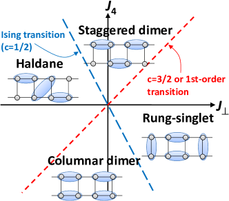
Figure 13: (Color online) Ground-state phase diagram of the spin ladder (38) in the weak rung-coupling regime. There are two transition curves, $J_{4}\approx 2.05J_{\perp}$ and $J_{4}\approx-6.15J_{\perp}$. The former is $c=3/2$ or first-order type, while the latter is in the Ising universality class with $c=1/2$ (see the text).

Finally, we note that in the extremely weak rung-coupling limit, the coupling constants of vertex operators in Eq. (39) would be less valid since coefficients $\bar{a}$ and $d$ are determined from gaps induced by relatively large staggered field ($h_{s}/J=0.1$ or $0.3$) and dimerization ($\delta_{xy,z}=0.1$ or $0.3$), respectively. The true transition curves might somewhat deviate from our prediction (40). Our result is expected to be more reliable in a moderate rung-coupling regime. In fact, a numerical study in Ref. Nomura09, has shown that the phase boundary is located at $J_{4}/J_{\perp}\sim 2$ around $J_{\perp}/J=0.25$ (see Fig. 6 in Ref. Nomura09, ), being consistent with Eq. (40a). We stress that our coefficients $\bar{a}$ and $d$ provides an easy way of estimating the phase boundary although it is a rough approximation compared with other sophisticated strategies such as DMRG and renormalization-group calculations. If we replace the intrachain term in Eq. (38) with two $J$-$J_{2}$ chains (16), the intrachain marginal interaction omitted in Eq. (39) disappears. In this case, the prediction from the effective theory (39) becomes more reliable even in the weak rung-coupling limit $J_{\perp}/J,J_{4}/J\to 0$. From the data of the $J$-$J_{2}$ model in Tables 1 and 2, two transition curves in the modified ladder are

$$J_{4}\approx 0.69J_{\perp},$$ (42a)

$$J_{4}\approx -2.08J_{\perp}.$$ (42b)

IV.3 Optical response of dimerized spin chains

Optical responses in Mott insulators including multiferroic compounds have been investigated intensively. Quite recently, the authors in Ref. Katsura09, have theoretically studied the optical conductivity in a 1D ionic-Hubbard type Mott insulator with Peierls instability, whose strong coupling limit is equal to a spin-$\frac{1}{2}$ dimerized Heisenberg chain, ${\cal H}^{{\rm XXX}-\delta}$. The results in Ref. Katsura09, would be relevant to, for example, organic Mott insulators such as TTF-BA. Kagawa10 In this system, the uniform electric polarization $P$ along the 1D chain is shown to be proportional to the dimer operator:

$$P=ga\sum_{j}(-1)^{j}{\boldsymbol{S}}_{j}\cdot{\boldsymbol{S}}_{j+1},$$ (43)

where $g$ is the coupling constant between the polarization and dimer operators. Therefore, $P$ can be bosonized as

$$P\approx 3dg\int dx\sin(\sqrt{4\pi}\phi(x))+\cdots,$$ (44)

with $d_{xy}=2d$ and $d_{z}=d$. From Eq. (44), one can calculate $P$ and related observables by means of the bosonization for the dimerized spin chain. It has been shown that the spin-singlet excitation, i.e., the breather with mass $E_{B_{2}}$, is observed as the lowest-frequency sharp peak in the optical conductivity measurements. Since the mass $E_{B_{2}}$ is evaluated from the sine-Gordon theory as

$$E_{B_{2}}/J=\sqrt{3}E_{S}/J=2.924\delta^{2/3},$$ (45)

we can extract the value of $\delta$ from the peak position of the optical conductivity. The exact expectation value of vertex operators in the sine-Gordon model has been predicted in Ref. Lukyanov97, . According to it, the polarization density is calculated to be

$$\langle P\rangle/L=({\cal A}/3)^{3/2}(E_{S}a/v)^{1/2}3dg,$$ (46)

with ${\cal A}\approx 3.041$ and $L$ being the chain length. This provides an experimental way of estimating the coupling constant $g$, which is usually difficult to determine in other multiferroic compounds.

V Conclusions

We have numerically evaluated coefficients of bosonized dimer and spin operators in spin-$\frac{1}{2}$ XXZ model (1) and $J$-$J_{2}$ model (16), by using the correspondence between the excitation gap of deformed models with dimerization (or with staggered Zeeman term) and the gap formula for the sine-Gordon theory. This is a new strategy relying on a solid relationship between the lattice models and their low-energy effective theories. Our numerical approach is relatively easy compared with another method based on DMRG, developed in Refs. Hikihara98, ; Hikihara04, , although the accuracy is expected to be better in the latter method. The obtained coefficients are summarized in Tables 1 and 2 and Fig. 4. In addition to these coefficients, we have pointed out a dangerous nature of applying the correlation amplitude (29) as coefficients of bosonized spin operators near the $SU(2)$-symmetric point $\Delta_{z}=1$ in Sec. III.5. Furthermore, we have also used the formula for ground-state energy of sine-Gordon model to calculate the same dimer coefficients in Sec. III.6. We conclude that the excitation-gap formula (11) is more suitable than the ground-state energy formula (12) for determining coefficients of bosonized operators.

Physical quantities associated with dimer and spin operators can be evaluated accurately by utilizing the dimer and spin coefficients. As examples, we have determined ground-state phase diagrams of dimerized spin chains in a uniform field and a two-leg spin ladder with a four-spin interaction in Sec. IV. In addition, we have shown how to estimate the electromagnetic coupling constant and the strength of the dimerization from the optical observables in a ferroelectric dimerized spin chain. These applications clearly indicate high potential of the data in Tables 1 and 2.

An interesting future direction is to apply a similar method to other 1D systems including fermion and boson models. Our method in this paper can be applied to lattice systems which have a well-established low-energy effective theory, in principle.

- (1) T. Giamarchi, Quantum Physics in One Dimension (Oxford University Press, New York, 2004).
- (2) I. Affleck, in Fields, Strings and Critical Phenomena, LesHouches, Session XLIX, edited by E. Brézin and J. Zinn-Justin (Elsevier, Amsterdam, 1989), p. 564.
- (3) V. E. Korepin, N. M. Bogoliubov, and A. G. Izergin, Quantum Inverse Scattering Method and Correlation Functions (Cambridge University Press, Cambridge, England, 1993).
- (4) M. Takahashi, Thermodynamics of One-Dimensional Solvable Models (Cambridge University Press, Cambridge, England, 1999).
- (5) A. O. Gogolin, A. A. Nersesyan, and A. M. Tsvelik, Bosonization and Strongly Correlated Systems (Cambridge University Press, Cambridge, England, 1998).
- (6) A. M. Tsvelik, Quantum Field Theory in Condensed Matter Physics, 2nd ed. (Cambridge University Press, Cambridge, England, 2003).
- (7) P. D. Francesco, P. Mathieu, and D. Sénéchal, Conformal Field Theory (Springer-Verlag, New York, 1997).
- (8) F. C. Alcaraz and A. L. Malvezzi, J. Phys. A, 28, 1521 (1995).
- (9) M. Oshikawa and I. Affleck, Phys. Rev. Lett. 79, 2883 (1997).
- (10) I. Affleck and M. Oshikawa, Phys. Rev. B 60, 1038 (1999).
- (11) F. H. L. Essler and A. M. Tsvelik, Phys. Rev. B 57, 10592 (1998).
- (12) I. Kuzmenko and F. H. L. Essler, Phys. Rev. B 79, 024402 (2009).
- (13) F. D. M. Haldane, Phys. Rev. B 25, 4925 (1982).
- (14) T. Papenbrock, T. Barnes, D. J. Dean, M. V. Stoitsov, and M. R. Strayer, Phys. Rev. B 68, 024416 (2003).
- (15) E. Orignac, Eur. Phys. J. B 39, 335 (2004).
- (16) D. G. Shelton, A. A. Nersesyan, and A. M. Tsvelik, Phys. Rev. B 53, 8521 (1996).
- (17) E. H. Kim, G. Fáth, J. Sólyom, and D. J. Scalapino, Phys. Rev. B 62, 14965 (2000).
- (18) O. A. Starykh and L. Balents, Phys. Rev. Lett. 93, 127202 (2004).
- (19) M. Kohno, O. A. Starykh, and L. Balents, Nat. Phys. 3, 790 (2007).
- (20) O. A. Starykh and L. Balents, Phys. Rev. Lett. 98, 077205 (2007).
- (21) S. Lukyanov and A. B. Zamolodchikov, Nucl. Phys. B, 493, 571 (1997).
- (22) S. Lukyanov, Phys. Rev. B 59, 11163 (1999).
- (23) S. Lukyanov, Nucl. Phys. B 654, 323 (2003).
- (24) T. Hikihara and A. Furusaki, Phys. Rev. B 58, R583 (1998).
- (25) T. Hikihara and A. Furusaki, Phys. Rev. B 69, 064427 (2004); cond-mat/0310391.
- (26) F. H. L. Essler and R. M. Konik, arXiv:cond-mat/0412421.
- (27) S. Lukyanov, Nucl. Phys. B 522, 533 (1998).
- (28) D. C. Cabra, A. Honecker and P. Pujol, Phys. Rev. B 58, 6241 (1998).
- (29) A. B. Zamolodchikov, Int. J. Mod. Phys. A, 10, 1125 (1995).
- (30) D. C. Dender, P. R. Hammar, D. H. Reich, C. Broholm, and G. Aeppli, Phys. Rev. Lett. 79, 1750 (1997).
- (31) K. Okamoto and K. Nomura, Phys. Lett. A 169, 433 (1992).
- (32) J. L. Cardy, J. Phys. A : Math. Gen., 17, L385 (1984).
- (33) J. L. Cardy, Nucl. Phys. B, 270, 186 (1986).
- (34) J. L. Cardy, J. Phys. A, 19, L1093 (1986).
- (35) D. Shanks, J. Math. Phys. (Cambridge, Mass.), 34, 1 (1955).
- (36) K. Nomura, Phys. Rev. B 48, 16814 (1993).
- (37) I. Affleck, J. Phys. A : Math. Gen. 31, 4573 (1998).
- (38) K. Okamoto and T. Nakamura, J. Phys. A, 30, 6287 (1997).
- (39) C. N. Yang and C. P. Yang, Phys. Rev. 150, 321 (1966).
- (40) A. A. Nersesyan and A. M. Tsvelik, Phys. Rev. Lett. 78, 3939 (1997).
- (41) M. Takahashi, J. Phys. C 10, 1289 (1977).
- (42) A. H. MacDonald, S. M. Girvin, and D. Yoshioka, Phys. Rev. B 37, 9753 (1988).
- (43) A. K. Kolezhuk and H.-J. Mikeska, Phys. Rev. Lett. 80, 2709 (1998).
- (44) K. Hijii and K. Nomura, Phys. Rev. B 80, 014426 (2009).
- (45) P. Lecheminant, A. O. Gogolin, and A. A. Nersesyan, Nucl. Phys. B 639, 502 (2002).
- (46) M. Nakamura, Physica B 329-333, 1000 (2003).
- (47) H. Katsura, M. Sato, T. Furuta, and N. Nagaosa, Phys. Rev. Lett. 103, 177402 (2009).
- (48) F. Kagawa, S. Horiuchi, M. Tokunaga, J. Fujioka and Y. Tokura, Nat. Phys. 6, 169 (2010).