A Short Tale of Long Tail Integration

Abstract

Integration of the form $\int_{a}^{\infty}{f(x)w(x)dx}$, where $w(x)$ is either $\sin(\omega{\kern 1.0pt}x)$ or $\cos(\omega{\kern 1.0pt}x)$, is widely encountered in many engineering and scientific applications, such as those involving Fourier or Laplace transforms. Often such integrals are approximated by a numerical integration over a finite domain $(a,\,b)$, leaving a truncation error equal to the tail integration $\int_{b}^{\infty}{f(x)w(x)dx}$ in addition to the discretization error. This paper describes a very simple, perhaps the simplest, end-point correction to approximate the tail integration, which significantly reduces the truncation error and thus increases the overall accuracy of the numerical integration, with virtually no extra computational effort. Higher order correction terms and error estimates for the end-point correction formula are also derived. The effectiveness of this one-point correction formula is demonstrated through several examples.

Keywords: numerical integration, Fourier transform, Laplace transform, truncation error.

1 Introduction

Integration of the form $\int_{a}^{\infty}{f(x)w(x)dx}$, where $w(x)$ is either $\sin(\omega{\kern 1.0pt}x)$ or $\cos(\omega{\kern 1.0pt}x)$, is widely encountered in many engineering and scientific applications, such as those involving Fourier or Laplace transforms. Often such integrals are approximated by numerical integrations over a finite domain $(a,\,b)$, resulting in a truncation error $\int_{b}^{\infty}{f(x)w(x)dx}$, in addition to the discretization error. One example is a discrete Fourier transform (DFT), where there is a truncation error due to cut-off in the tail, in addition to the discretization error.

In theory the cut-off error can always be reduced by extending the finite domain at the expense of computing time. However, in many cases a sufficiently long integration domain covering a very long tail can be computationally expensive, such as when the integrand $f(x)$ itself is a semi-infinite integration (e.g. forward Fourier or Laplace transform), or when the integrand decays to zero very slowly (e.g. a heavy tailed density or its characteristic function). Much work has been done to directly compute the tail integration in order to reduce the truncation error. Examples include nonlinear transformation and extrapolation (Wynn 1956, Alaylioglu et al 1973, Sidi 1980, 1982, 1988, Levin and Sidi 1981) and application of special or generalized quadratures (Longman 1956, Hurwitz and Zweifel 1956, Bakhvalov and Vasileva 1968, Piessens 1970, Piessens and Haegemans 1973, Patterson 1976, Evans and Webster 1997, Evans and Chung 2007), among many others. This paper describes a very simple, perhaps the simplest, end-point correction to account for the tail integration over the entire range $(b,\infty)$. The treatment of the tail reduces the usual truncation error significantly to a much smaller discrete error, thus increasing overall accuracy of the integration, while requiring virtually no extra computing effort. For the same accuracy, this simple tail correction allows a much shorter finite integration domain than would be required otherwise, thus saving computer time while avoiding extra programming effort. To our knowledge this result is not known in the literature and we believe it deserves to be published for its elegant simplicity and broad applicability. Though it is possible that our formula is a rediscovery of a very old result hidden in the vast literature related to numerical integration.

The paper is organized as follows. In Section 2, we derive the tail integration approximation and its analytical error. A few examples are shown to demonstrate the effectiveness of the tail integration approximation in Section 3. Concluding remarks are given in Section 4.

2 Tail integration

Consider integration $\int_{a}^{\infty}{f(x)\sin(\omega{\kern 1.0pt}x)dx}$. Without loss of generality, we assume $\omega=1$ (a change of variable $y=\omega{\kern 1.0pt}x$ results in the desired form). For $\int_{a}^{\infty}{f(x)\cos(\omega{\kern 1.0pt}x)dx}$ the derivation procedure and the resulting formula are very similar. In the following, we assume that

• The integral $\int_{a}^{\infty}{f(x)\sin(\omega{\kern 1.0pt}x)dx}$ exists;

• All derivatives $f^{(k)}(x)$ exist and $\to 0$ as $k\to\infty$.

2.1 Piecewise linear approximation

The truncation error of replacing $\int_{a}^{\infty}{f(x)\sin(x)dx}$ by $\int_{a}^{b}{f(x)\sin(x)dx}$ is simply the tail integration

$$I_{T}=\int\limits_{b}^{\infty}{f(x)\sin(x)dx}.$$ (1)

For higher accuracy, instead of increasing truncation length at the cost of computing time, we propose to compute the tail integration $I_{T}$ explicitly by a very economical but effective simplification. Assume $f(x)$ approaches zero as $x\to\infty$ and the truncation point $b$ can be arbitrarily chosen in a numerical integration. Let $b=N\pi$, where $N$ is some large integer. Dividing integration from $N\pi$ to $\infty$ into cycles with an equal length of $\pi$ yields

$$\int\limits_{N\pi}^{\infty}{f(x)\sin(x)dx}=\sum\limits_{k=0}^{\infty}{I_{k}{\kern 1.0pt},\quad I_{k}=\int\limits_{(N+k)\pi}^{(N+k+1)\pi}{f(x)\sin(x)dx}}.$$ (2)

Now assume that $f(x)$ is piecewise linear within each $\pi$-cycle, so that each of the integrals $I_{k}$ in (2) can be computed exactly. That is, in the range $\left[{(N+k)\pi,(N+k+1)\pi}\right]$, we assume that $f(x)$ is approximated by

$$f(x)\approx f_{k}+\frac{x-(N+k)\pi}{\pi}(f_{k+1}-f_{k}),$$ (3)

where $f_{k}=f((N+k)\pi)$. Substitute (3) into (2), then analytical integration by parts of each $I_{k}$ in (2) gives

$$\int\limits_{N\pi}^{\infty}f(x)\sin(x)dx=\sum\limits_{k=0}^{\infty}{I_{k}}\approx\sum\limits_{k=0}^{\infty}{(-1)^{N+k}(f_{k}+f_{k+1})}=(-1)^{N}f_{0}=(-1)^{N}f(N\pi).$$ (4)

This elegant result given by (4) means that we only need to evaluate the integrand $f(x)$ at one single point $x=N\pi$ (the truncation point) for the entire tail integration, replacing the truncation error with a much smaller round-off error. As will be demonstrated later, this one-point formula for the potentially demanding tail integration is remarkably effective in reducing the truncation error caused by ignoring $I_{T}$.

2.2 Higher order correction terms and error estimates

Formula (4) can be derived more generally through integration by parts, and a recursive deduction gives us higher order correction terms and thus error estimates. Integrating (1) by parts with $b=N\pi$, we have

$$\int\limits_{N\pi}^{\infty}{f(x)\sin(x)dx=\,}(-1)^{N}f(N\pi)+\int\limits_{N\pi}^{\infty}{f^{(1)}(x)\cos(x)dx},$$ (5)

where $f^{(1)}(x)=df(x)/dx$. If we assume $f(x)$ is linear within each $\pi$-cycle in the tail, then the integration $\int_{N\pi}^{\infty}{f^{(1)}(x)\cos(x)dx}$ vanishes, because within each $\pi$-cycle $f^{(1)}(x)$ is constant from the piecewise linear assumption and $\int_{k\pi}^{(k+1)\pi}{\cos(x)dx}=0$ for any integer $k$, and $f^{(1)}(\infty)\to 0$ as $f(\infty)\to 0$. Thus, under the piecewise linear assumption, (5) and (4) are identical. Continuing with integration by parts in (5) and noting $f^{(1)}(x)\to 0$ at infinity, we further obtain

$$\int\limits_{N\pi}^{\infty}{f(x)\sin(x)dx=}\,(-1)^{N}f(N\pi)-\int\limits_{N\pi}^{\infty}{f^{(2)}(x)\sin(x)dx},$$ (6)

where $f^{(2)}(x)=d^{2}f(x)/dx^{2}$. Equation (6), as well as (5), is exact – no approximation is involved. The recursive pattern in (6) is evident. If we now assume that the second derivative $f^{(2)}(x)$ is piecewise linear in each $\pi$-cycle in the tail, then (6) becomes

$$\int\limits_{N\pi}^{\infty}{f(x)\sin(x)dx\approx\,}(-1)^{N}\left({f(N\pi)-f^{(2)}(N\pi)}\right).$$ (7)

With the additional correction term, (7) is more accurate than (4). In general, without making any approximation, from the recursive pattern of (6) we arrive at the following expression for the tail integral

$$\int\limits_{N\pi}^{\infty}{f(x)\sin(x)dx}=(-1)^{N}f(N\pi)+\sum\limits_{i=1}^{k-1}{(-1)^{N+i}f^{(2i)}(N\pi)}+(-1)^{k}\int\limits_{N\pi}^{\infty}{f^{(2k)}(x)\sin(x)dx},$$ (8)

where $k\geq 1$, $f^{(2k)}(N\pi)$ is the 2$k$-th order derivative of $f(x)$ at the truncation point. As will be shown later with examples, typically the first few terms from (8) are sufficiently accurate. The error in using formula (4) is readily obtained from (8)

$$\varepsilon_{T}=\sum\limits_{i=1}^{k-1}{(-1)^{N+i}f^{(2i)}(N\pi)}+(-1)^{k}\int\limits_{N\pi}^{\infty}{f^{(2k)}(x)\sin(x)dx},$$ (9)

In deriving (8), we have assumed all derivatives exist and $f^{(k)}(\infty)=0$. Under certain conditions, the infinite series in (8) and (9) represents the integral asymptotically as $N\to\infty$, i.e. we have the asymptotic expansion

$$\int\limits_{N\pi}^{\infty}{f(x)\sin(x)dx}\sim\sum\limits_{i=0}^{\infty}{(-1)^{N+i}f^{(2i)}(N\pi)}\;\;\;\mbox{as}\;\;\;N\to\infty$$

For example, if we assume that, for some $\gamma<0$,

$$f^{(m)}(x)=O(x^{\gamma-m})\;\;\;\mbox{as}\;\;\;N\to\infty,\;\;\;m=0,1,2,...,$$

then the integral term on the right-hand side of (8) can be bounded by $C_{k}N^{\gamma-2k+1}$ as $N\to\infty$, for some positive constant $C_{k}$, and the series converges to the integral.

The derivatives approaching zero as $x\to\infty$ is a consequence of the existence of integral (1). Otherwise, if $f^{(1)}(\infty)\neq 0$, integral (1) does not exist, which is evident form (5). Applying this argument recursively, all derivatives $f^{(k)}(\infty)=0$, if they exist. Obviously if $f(x)$ is a power function (e.g. $1/\sqrt{x}$), the ratio $f^{(1)}(x)/f(x)$ is of the order $1/x$ as $x\to\infty$, so is the ratio $f^{(k+1)}(x)/f^{(k)}(x)$. This implies that, for a power-like function, each error term in (9) decreases by two orders of magnitude from its preceding term as the index number $k$ increases by one.

Remark. Note that there is no truncation error in (4) and the error is a discretization error in nature. In theory, the tail integration error can be estimated by (9). In practice, however, derivatives of integrand at the truncation point may only be evaluated numerically. The assumption of piecewise linearity, although reasonable for $f(x)$ at large $x$, may appear to be rather crude for a high precision computation. However, we recall that we are only trying to reduce the already small truncation error $I_{T}$ and a reasonable approximation in $I_{T}$ could lead to significant improvement in the overall accuracy of integration. For example, suppose a relative error of 1% due to ignoring truncation and 10% error in evaluating the tail integration using the very simple formula (4). The overall accuracy with this tail integration added is now improved from 1% to 0.1% (1% times 10%). This improvement by an order of magnitude is achieved by simply evaluating the integrand at the truncation point. The assumption of a piecewise linearity applies to a broad range of functions, thus the special tail integration approximation can have a wide application. Note, piecewise linear assumption does not even require monotonicity - $f(x)$ can be oscillating, as long as its frequency is relatively small compared with the principal cycles in $\sin(x)$, as demonstrated in one of the examples below.

If the oscillating factor is $\cos(x)$ instead of $\sin(x)$, we can still derive a one-point formula similar to (4) by starting the tail integration at $(N-1/2)\pi$ instead of $N\pi$. In this case, the tail integration is

$$\int\limits_{(N-1/2)\pi}^{\infty}{f(x)\cos(x)dx\approx}(-1)^{N}f\left({(N-1/2)\pi}\right).$$ (10)

Also, the tail integration approximation can be applied to the left tail (integrating from $-\infty$ to $-N\pi)$ as well, if such integration is required.

It is known from the literature that truncation is better at extrema of the oscillatory part than at the zeros (Lyness 1986, Espelid and Overholt 1994 and Sauter 2000). Truncating at $x_{T}=(N-1/2)\pi$, the extrema for $sin(x)$, we obtain an expression for the tail integration or the truncation error similar to (8)

$$\int\limits_{x_{T}}^{\infty}{f(x)\sin(x)dx} = (-1)^{N}f^{(1)}(x_{T})+\sum\limits_{i=1}^{k-1}{(-1)^{N+i}f^{(2i+1)}(x_{T})}$$ (11)

$$+(-1)^{k}\int\limits_{x_{T}}^{\infty}{f^{(2k)}(x)\sin(x)dx}.$$

The leading term of the truncation error is now $f^{(1)}(x_{T})$ in (11), compared with $f(x_{T}+1/2\pi)$ in (8). Assuming $|f^{(1)}(x_{T})/f(x_{T}+1/2\pi)|<1$ for some large $x_{T}$, e.g. when $f(x)$ is a power-like function, then it is obvious truncation at extrema has a smaller truncation error. However, our formula is about the reduction of the truncation error by including an approximation of the tail integration. If truncation is done at $x=(N-1/2)\pi$ instead of $x=N\pi$, then the first correction term will be $(-1)^{N+1}f^{(1)}((N-1/2)\pi)$, involving the first derivative of $f(x)$. In many important applications the first derivative of $f(x)$ cannot be evaluated accurately. For example, when inverting a characteristic function of a compound distribution, $f(x)$ itself is a semi-infinite integration of an oscillatory function, which could only be obtained numerically. Taking finite difference of a numerically evaluated function will in general reduce the accuracy by an order of magnitude. So for general purposes the truncation is chosen at the zeros, i.e. at $x=N\pi$.

Of course, if derivative of $f(x)$ is in closed form and can be accurately evaluated, truncation and correction at extrema will indeed be more accurate, with a leading error term of $f^{(3)}(x_{T})$. But we could also include the second derivative term for the truncation at zeros, with a leading error term of $f^{(4)}(x_{T})$, and so on. In general when higher order derivatives can be computed precisely, then one can include some higher order terms to reduce truncation error further and it does not matter much whether the truncation is done at extrema or at zeros.

3 Examples of tail integration

The effectiveness of the above tail integration approximation is now demonstrated in a few examples. Introduce the following notations

$$I_{E} = \int_{0}^{\infty}{f(x)\sin(x)dx},$$

$$\tilde{I}(N\pi) = \int_{0}^{\pi{\kern 1.0pt}N}{f(x)\sin(x)dx},$$

$$I_{T}(N\pi) = \int_{\pi{\kern 1.0pt}N}^{\infty}{f(x)\sin(x)dx}.$$

In all the following examples the exact semi-infinite integration $I_{E}$ is known in closed form, and its truncated counterpart $\tilde{I}(N\pi)$ is either known in closed form or can be computed accurately. For simplicity in all the examples $N$ is taken to be an even number, i.e $(-1)^{N}=1$. The exact tail integration $I_{T}(N\pi)$ can be computed from $I_{T}(N\pi)=I_{E}-\tilde{I}(N\pi)$. We compare $\tilde{I}(N\pi)+f(N\pi)$ with $\tilde{I}(N\pi)$ and compare both of them with the exact semi-infinite integration $I_{E}$. The error reduction can be quantified by comparing the “magic” point value given by formula (4) with the exact tail integration $I_{T}(N\pi)$. Also note that the analytic formula for the error of using (4), $\varepsilon_{T}=I_{E}-[\tilde{I}(N\pi)+f(N\pi)]$, is given by (9).

Example 1: $f(x)=e^{-\alpha x},\,\;(\alpha>0).$

In this example, the closed form results are

$$I_{E}=\int\limits_{0}^{\infty}{e^{-\alpha x}\sin(x)dx=}\frac{1}{1+\alpha^{2}},\quad\tilde{I}(N\pi)=\int\limits_{0}^{N\pi}{e^{-\alpha x}\sin(x)dx=}\frac{1-e^{-\alpha\,N\pi}}{1+\alpha^{2}}.$$

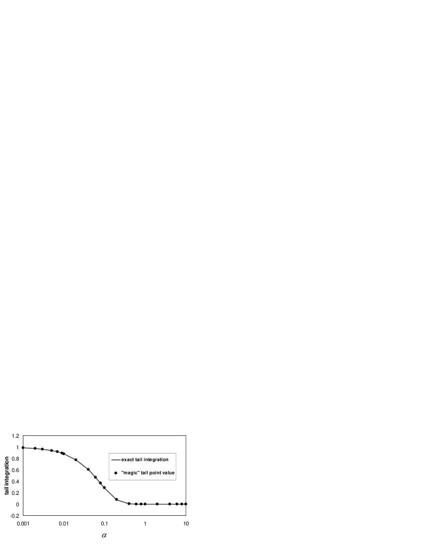
Figure 2: Comparison between the exact tail integration $\int_{\pi N}^{\infty}{f(x)\sin(x)dx}$ and simple one-point approximation $f(N\pi)$ from formula (4), when $f(x)=e^{-\alpha\,x}$ and $N=4$.

Figure 1 compares the “magic” point value $f(N\pi)$ representing simplified tail integration with the exact tail integration $I_{T}(N\pi)=I_{E}-\tilde{I}(N\pi)$ as functions of parameter $\alpha$ for $N=10$, i.e. the truncated lengths $l_{T}=10\pi$. The figure shows that a simple formula (4) matches the exact semi-infinite tail integration surprisingly well for the entire range of parameter $\alpha$. Corresponding to Figure 1, the actual errors of using formula (4) are shown in Table 1, in comparison with the truncation errors without applying the correction term given by (4). Figure 2 shows the same comparison at an even shorter truncated length of $4\pi$. The error of using (4) is $\left|\varepsilon_{T}\right|={\alpha^{2}\exp(-\alpha\pi N)/(1+\alpha^{2})}$.

If $\alpha$ is large, the function $f(x)=e^{-\alpha x}$ is “short tailed” and it goes to zero very fast. The absolute error $\left|\varepsilon_{T}\right|$ is very small even at $N=4$. The relative error (against the already very small tail integration), given by $\left|\varepsilon_{T}\right|/\left|{I_{E}-\tilde{I}(2N\pi)}\right|=\alpha^{2}$, is actually large in this case. But this large relative error in the tail approximation does not affect the high accuracy of the approximation for the whole integration. What is important is the error of the tail integration relative to the whole integration value. Indeed, relative to the exact integration, the error of using (4) is $\left|\varepsilon_{T}\right|/\left|{I_{E}}\right|=\alpha^{2}\exp(-\alpha\pi N)$, which is about $2.7\times 10^{-53}$ at $N=4$. The condition $f^{(k)}(x)\to 0$ as $k\to\infty$ is not satisfied in this case if $\alpha>1$. However, as discussed above, the application of formula (4) does not cause any problem.

For a small value of parameter $\alpha$, the truncation error will be large unless the truncated length is very long. For instance, with $\alpha=0.01$ the truncation error (if ignore the tail integration) is more than 70% at $l_{T}=10\pi$ ($N=10$, as the case in Figure 1), and it is more than 88% at $l_{T}=4\pi$ ($N=4$, as the case in Figure 2). On the other hand, if we add the “magic” value from formula (4) to approximate the tail integration, the absolute error of the complete integration $\left|\varepsilon_{T}\right|$ due to this approximation is less than 0.01%, and the relative error is $\left|\varepsilon_{T}\right|=\alpha^{2}=0.01\%$ at both $l_{T}=10\pi$ and $l_{T}=4\pi$. In other words, by including this one-point value, the accuracy of integration has dramatically improved by several orders of magnitude at virtually no extra cost, compared with the truncated integration. For the truncated integration $\tilde{I}(N\pi)$ to have similar accuracy as $\tilde{I}(4\pi)+f(4\pi)$, we need to extend the truncated length from $4\pi$ to $300\pi$ for this heavy tailed integrand.

Example 2: $f(x)=1/\sqrt{x}$ .

This example has a heavier tail than the previous one. Here, we have closed form for $I_{E}$, but not for $\tilde{I}$ or $I_{T}$,

$$I_{E}=\int\limits_{0}^{\infty}{\frac{\sin(x)}{\sqrt{x}}dx=}\sqrt{\frac{\pi}{2}},\quad\tilde{I}(N\pi)=\int\limits_{0}^{N\pi}{\frac{\sin(x)}{\sqrt{x}}dx}.$$

$\tilde{I}$ or $I_{T}$ can be accurately computed by adaptive integration functions available in many numerical packages. Here we used IMSL function based on the modified Clenshaw-Curtis integration method (Clenshaw and Curtis 1960; Piessens, Doncker-Kapenga, Überhuber and Kahaner 1983).

Figure 3 compares the “exact” tail integration $I_{T}(N\pi)=\int_{N\pi}^{\infty}{\sin(x)/\sqrt{x}dx}$ with the one-point value $f(N\pi)$. Again the one-point approximation does an extremely good job. Even at the shortest truncation length of just $2\pi$ the one-point approximation is very close to the exact semi-infinite tail integration. Applying the analytical error formula (9) to $f(x)=1/\sqrt{x}$, we have

$$\varepsilon_{T}=\sum\limits_{k=1}^{\infty}{(-1)^{k}\frac{1\times 3\times...\times(4k-1)}{2^{2k}x^{(4k+1)/2}}}.$$

Taking the first three leading terms we get $\varepsilon_{T}\approx-\mbox{0.00}6\mbox{95}$ at $N=2$ and $\varepsilon_{T}\approx-\mbox{2.392}\times\mbox{10}^{-5}$ at $N=20$. The relative error $\left|\varepsilon_{T}\right|/I_{E}(2N\pi)$ is about 1% at $N=2$ and it is about 0.002% at $N=20$. Apparently, if the extra correction term $f^{(2)}(N\pi)$ is included as in (7), the error $\varepsilon_{T}$ reduces further by an order of magnitude at $N=2$ and by several orders of magnitude at $N=20$. Corresponding to Figure 3, the actual errors of using formula (4) are shown in Table 2, in comparison with the truncation errors without applying the correction term given by (4).

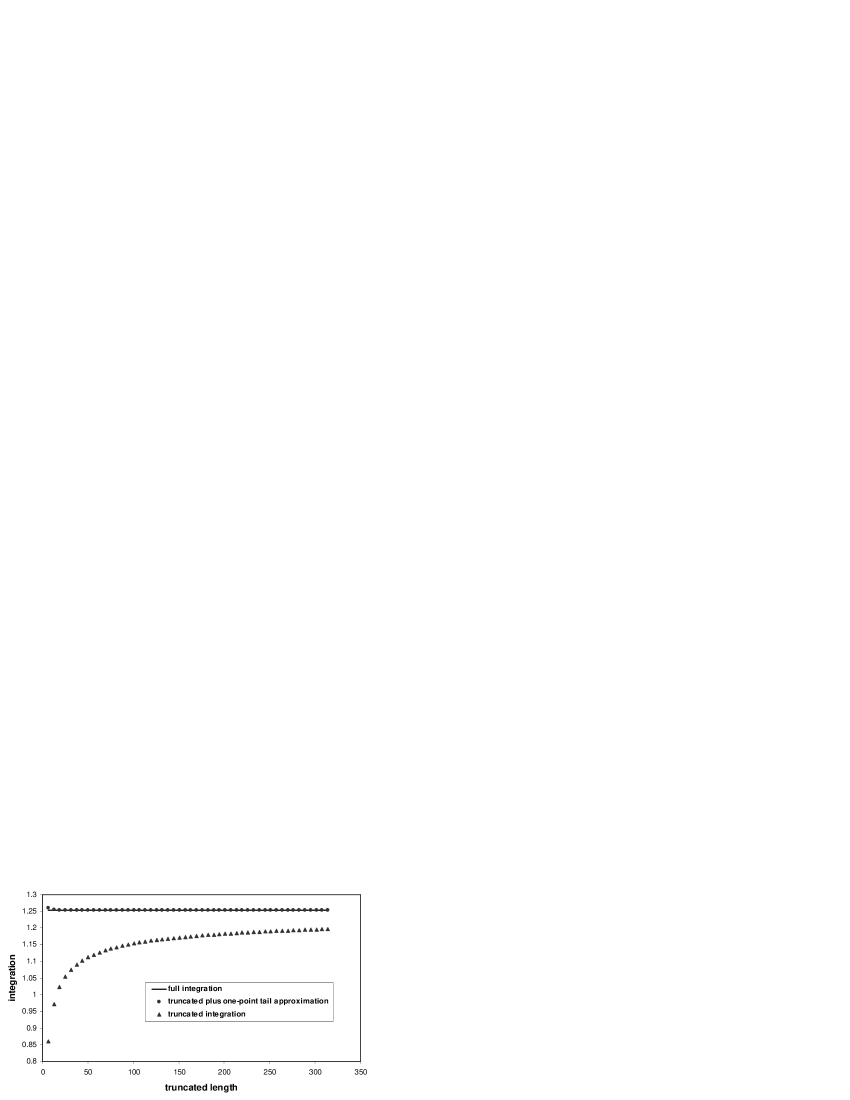
Figure 4: Comparison between truncated integration $\tilde{I}(N\pi)=\int_{0}^{\pi N}{f(x)\sin(x)dx}$ and the truncated integration plus the one-point approximation of tail integration, $\tilde{I}(N\pi)+f(N\pi)$, as functions of the truncated length $l_{T}=N\pi,\;4\leq N\leq 100$, where $f(x)=1/\sqrt{x}$. The solid line represents the exact value of the full integration without truncation error, $I_{E}=\tilde{I}(\infty)=\sqrt{\pi/2}$.

Figure 4 shows the truncated integration $\tilde{I}(N\pi)$ and the truncated integration with the tail modification (4) added, i.e. $\tilde{I}+f(N\pi)$, along with the correct value of the full integration $I_{E}=\sqrt{\pi/2}$. The contrast between results with and without the one-point tail approximation is striking. At the shortest truncation length of $2\pi$ ($N=2)$, the relative error due to truncation for the truncated integration $(I_{E}-\tilde{I}(N\pi))/I_{E}$ is more than 30%, but with the tail approximation added, the relative error $(I_{E}-\tilde{I}(N\pi)-f(N\pi))/I_{E}$ reduces to 0.5%. At $100\pi$, the largest truncation length shown in Figure 4, the relative error due to truncation is still more than 4%, but after the “magic” point value is added the relative error reduces to less than $0.5\times 10^{-6}$.

Another interesting way to look at these comparisons, which is relevant for integrating heavy tailed functions, is to consider the required truncation length for the truncated integration to achieve the same accuracy as the one with the “magic” value added. For the truncated integration $\tilde{I}(N\pi)$ to achieve the same accuracy of $\tilde{I}(2\pi)+f(2\pi)$ (integration truncated at one-cycle plus the “magic point value), we need to extend the integration length to $7700\pi$. For $\tilde{I}(N\pi)$ to achieve the same accuracy of $\tilde{I}(100\pi)+f(100\pi)$, the integration length has to be extended to more than $10^{12}\pi$! On the other hand, if we add the tail approximation $f(7700\pi)$ to $\tilde{I}(7700\pi)$, the relative error reduces from 0.5% to less than $10^{-11}$! This error reduction requires no extra computing, since $f(7700\pi)$ is simply a number given by $1/\sqrt{7700\pi}$.

Example 3: $f(x)=\cos(\alpha x)/x,\;\alpha<1$.

We have remarked that the piecewise linear assumption does not require monotonicity, i.e. $f(x)$ can be oscillating, as long as its frequency is relatively small compared with the principal cycles. For example, when the function $f(x)$ is the characteristic function of a compound distribution, it oscillates with its frequency approaching zero in the long tail. In the current example with $f(x)=\cos(\alpha x)/x$, there is a closed form for $I_{E}$, but not for $\tilde{I}$ or $I_{T}$,

$$I_{E}=\int\limits_{0}^{\infty}{\frac{\cos(\alpha x)\sin(x)}{x}dx=}\frac{\pi}{2},\quad\tilde{I}(2N\pi)=\int\limits_{0}^{N\pi}{\frac{\cos(\alpha x)\sin(x)}{x}dx},\quad\alpha<1.$$

Figure 5 compares the “exact” tail integration $I_{T}(N\pi)$ with the one-point approximation $f(N\pi)$ for the case $\alpha=0.2$. Again the one-point approximation performs surprisingly well, despite $f(x)$ itself is now an oscillating function, along with the principal cycles in $\sin(x)$. The piecewise linearity assumption is apparently still valid for relatively mild oscillating $f(x)$. Corresponding to Figure 5, the actual errors of using formula (4) are shown in Table 3, in comparison with the truncation errors without applying the correction term given by (4). Not surprisingly, the errors are larger in comparison with those in examples 1 and 2, due to the fact that $f(x)$ now is itself an oscillating function. Still, Table 3 shows the truncation error is reduced by an order of magnitude after applying the simple formula (4).

Figure 6 compares the truncated integration $\tilde{I}(N\pi)$ against $\tilde{I}+f(N\pi)$, along with the correct value of the full integration $I_{E}=\pi/2$. At truncation length $6\pi$, the shortest truncation length shown in Figures 5 and 6, the relative error $\left|\varepsilon_{T}\right|/I_{E}$ is less than 0.06% and it is less than 0.01% at $N=100$. In comparison, the truncated integration without the end point correction has relative error of 2.7% and 0.2%, respectively for those two truncation lengths. Applying the analytical error formula (9) to $f(x)=\cos(\alpha x)/x$ and noting $\sin(\alpha x)=0$ and $\cos(\alpha x)=1$ with $\alpha=0.2$ and $x=100\pi$, we obtain

$$\varepsilon_{T}\approx-\left({-\frac{\alpha^{2}}{x}+\frac{2}{x^{3}}}\right)+\left({\frac{\alpha^{4}}{x}-\frac{12\alpha^{2}}{x^{3}}+\frac{24}{x^{5}}}\right),\quad x=l_{T}=100\pi,$$

where only the first two leading terms corresponding to the 2^nd and 4^th derivatives are included, leading to $\varepsilon_{T}\approx 0.0001273+5.07749\times 10^{-6}$ at $N=50$ that agrees with the actual error. Similar to the previous example, if we include the extra correction term $f^{(2)}(N\pi)$, the error reduces further by two orders of magnitude at $N=100$.

The purpose of Example 3 is to show that the piecewise linear approximation in the tail could still be valid even if there is a secondary oscillation in $f(x)$, provided its frequency is not as large as the principal oscillator. If the parameter $\alpha$ is larger than one, then we can simply perform a change of variable with $y=\alpha x$ and integrate $(1/y)\sin(y/\alpha)\cos(y)$ in terms of $y$. Better still, for any value of $\alpha$, we can make use of the equality $\cos(\alpha x)\sin(x)=(\sin(x-\alpha x)+\sin(x+\alpha x))/2$ to get rid of the secondary oscillation altogether before doing numerical integration. In practice, the secondary oscillation often has a varying frequency with a slowly decaying magnitude, such as in the case of the characteristic function of a compound distribution with a heavy tail. In this case it might be difficult to effectively apply regular numerical quadratures in the tail integration, but the simple one-point formula (4) might be very effective.

All these examples show dramatic reduction in truncation errors if tail integration approximation (4) is employed, with virtually no extra cost. If the extra correction term $f^{(2)}(2N\pi)$ is included, i.e. using (7) instead of (4), the error is reduced much further.

4 Conclusions

We have derived perhaps the simplest but efficient tail integration approximation, first intuitively by piecewise linear approximation, then more generally through integration by parts. Analytical higher-order correction terms and thus error estimates are also derived. The usual truncation error associated with a finite length of the truncated integration domain can be reduced dramatically by employing the one-point tail integration approximation, at virtually no extra computing cost, so a higher accuracy is achieved with a shorter truncation length.

Under certain conditions outlined in the present study, the method can be used in many practical applications. For example, the authors have successfully applied the present method in computing heavy tailed compound distributions through inverting their characteristic functions, where the function $f(x)$ itself is a semi-infinite numerical integration (Luo, Shevchenko and Donnelly 2007).

Of course there are more elaborate methods in the literature which are superior to the present simple formula in terms of better accuracy and broader applicability, such as some of the extrapolation methods proposed by Wynn 1956 and by Sidi 1980, 1988. The merit of the present proposal is its simplicity and effectiveness - a single function evaluation for the integrand at the truncation point is all that is needed to reduce the truncation error, often by orders of magnitude. It can not be simpler than that. Also, in some applications the function $f(x)$ may not even exist in closed form, for instance when $f(x)$ is the characteristic function of some compound distributions as mentioned above, then $f(x)$ itself is a semi-infinite integration of a highly oscillatory function, which could only be obtained numerically. In such cases some of the other more sophisticated methods relying on a closed form of $f(x)$ may not be readily applicable.

5 Acknowledgement

We would like to thank David Gates, Mark Westcott and three anonymous refrees for many constructive comments which have led to significant improvements in the manuscript.

Table 1: Error of using formula (4), $\varepsilon_{T}$, in comparison with the truncation error $I_{T}$ if formula (4) is not applied, corresponding to Figure 1 in Example 1.

$\alpha$	$\varepsilon_{T}$	$I_{T}$
0.001	$9.4\times 10^{-7}$	0.9391
0.01	$5.3\times 10^{-5}$	0.5334
0.1	$1.8\times 10^{-5}$	0.0018
1	$2.6\times 10^{-28}$	$2.6\times 10^{-28}$
10	0.0	0.0

Table 2: Error of using formula (4), $\varepsilon_{T}$, in comparison with the truncation error $I_{T}$ if formula (4) is not applied, corresponding to Figure 3 in Example 2.

$x$	$\varepsilon_{T}$	$I_{T}$
$4\pi$	$1.0\times 10^{-3}$	0.2241
$10\pi$	$1.1\times 10^{-4}$	0.1422
$20\pi$	$1.9\times 10^{-5}$	0.1006
$50\pi$	$1.9\times 10^{-6}$	0.0637
$100\pi$	$3.4\times 10^{-7}$	0.0318

Table 3: Error of using formula (4), $\varepsilon_{T}$, in comparison with the truncation error $I_{T}$ if formula (4) is not applied, corresponding to Figure 5 in Example 3.

$x$	$\varepsilon_{T}$	$I_{T}$
$20\pi$	$4.2\times 10^{-4}$	0.0105
$40\pi$	$2.1\times 10^{-4}$	0.0053
$60\pi$	$1.4\times 10^{-4}$	0.0035
$80\pi$	$1.1\times 10^{-4}$	0.0026
$100\pi$	$8.4\times 10^{-5}$	0.0021

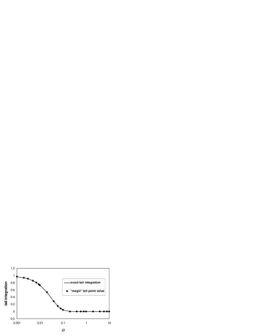
Figure 1: Comparison between the exact tail integration $\int_{\pi N}^{\infty}{f(x)\sin(x)dx}$ and simple one-point approximation $f(N\pi)$ from formula (4), when $f(x)=e^{-\alpha\,x}$ and $N=10$.

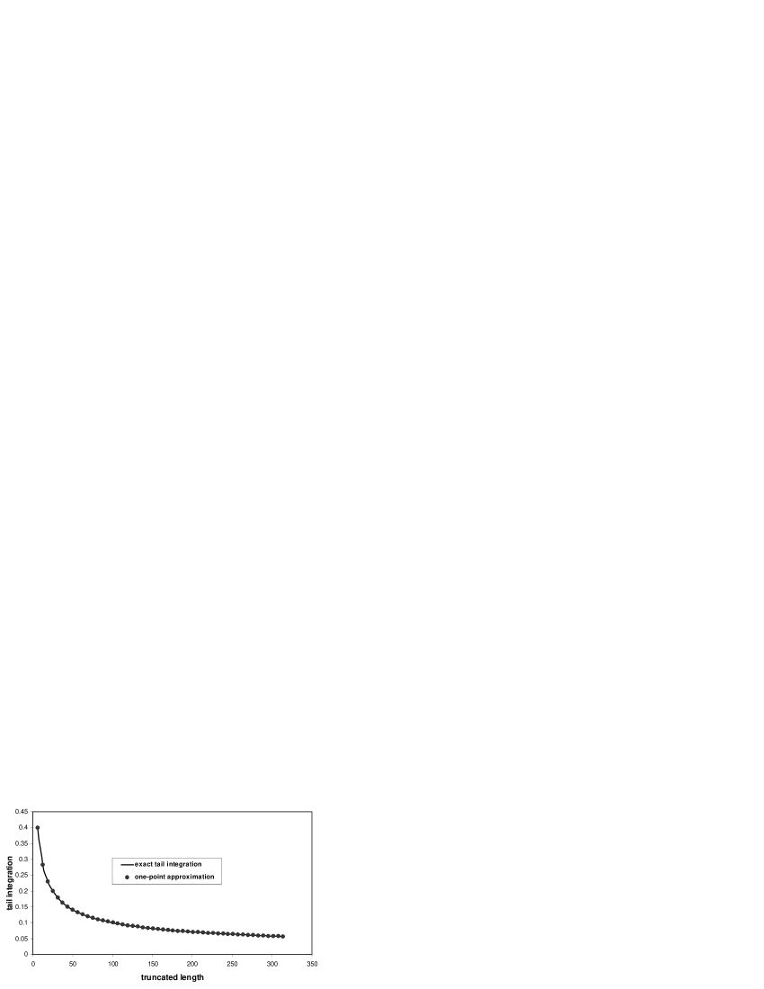
Figure 3: Comparison between exact tail integration $\int_{\pi N}^{\infty}{f(x)\sin(x)dx}$ and the simple one point approximation (4), $f(N\pi)$, as functions of truncated length $l_{T}=N\pi,\;4\leq N\leq 100$, when $f(x)=1/\sqrt{x}$.

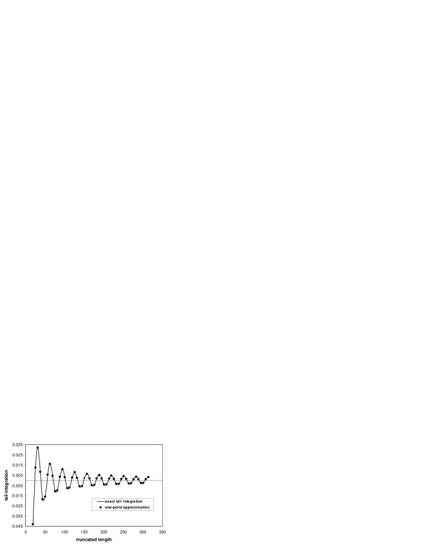
Figure 5: Comparison between exact tail integration $\int_{\pi N}^{\infty}{f(x)\sin(x)dx}$ and the simple one-point approximation (4), $f(N\pi)$, as functions of truncated length $l_{T}=N\pi,\;6\leq N\leq 100$, $f(x)=\cos(\alpha x)/x$, $\alpha=0.2$.

Figure 6: Comparison between truncated integration $\tilde{I}(N\pi)=\int_{0}^{\pi N}{f(x)\sin(x)dx}$ and the truncated integration plus the one-point approximation of tail integration, $\tilde{I}(N\pi)+f(N\pi)$, as functions of the truncated length $l_{T}=N\pi,\;6\leq N\leq 100$, where $f(x)=\cos(\alpha x)/x$, $\alpha=0.2$. The solid line represents the exact value of the full integration without truncation error, $I_{E}=\tilde{I}(\infty)=\pi/2$.

References

- [1] A. Alaylioglu, G. A. Evans, and J. Hyslop, The evaluation of oscillatory integrals with infinite limits, J. Comp. Phys, 13 (1973), 433–438.
- [2] N. S. Bakhvalov and L. G. Vasil’eva, Evaluation of integrals of oscillating functions by interpolation at nodes of gaussian quadratures, USSR Comp. Math. Math. Phys. 8 (1968), 241–249.
- [3] C. W. Clenshaw and A. R. Curtis, A method for numerical integration on an automatic computer, Num. Math 2 (1960), 197–205.
- [4] T. O. Espelid and K. J. Overholt, Dqainf: An algorithm for automatic integration of infinite oscillating tails, Numer. Algorithms 8 (1994), 83–101.
- [5] G. A. Evans and K. C. Chung, Evaluating infinite range oscillating integrals using generalized quadrature methods, Appl. Numer. Math. 57 (2007), 73–79.
- [6] G. A. Evans and J. R. Webster, A high order progressive method for the evaluation of irregular oscillating integrals, Appl. Numer. Anal. 23 (1997), 205–218.
- [7] H. Jr. Hurwitz and P. F. Zweifel, Numerical quadrature of fourier transform integrals, MTAC 10 (1956), 140–149.
- [8] D. Levin and A. Sidi, Two new classes of nonlinear transformations for accelerating the convergence of infinite integrals and series, Appl. Math. Comput. 9 (1981), 175–215.
- [9] I. M. Longman, Note on a method for computing infinite integrals of oscillatory functions, Camb. Phil. Soc. Proc. 52 (1956), 764.
- [10] X. Luo, P. V. Shevchenko, and J. Donnelly, Addressing impact of truncation and parameter uncertainty on operational risk estimates, The Journal of Operational Risk 2 (2007), 3–26.
- [11] J. Lyness and G. Hines, To integrate some infinite oscillating tails, ACM Trans. Math. software 12 (1986), 24–25.
- [12] T. N. L. Patterson, On high precision methods for the evaluation of fourier integrals with finite and infinite limits, Numer. Math. 27 (1976), 41–52.
- [13] R. Piessens, Gaussian quadrature fomulas for the integration of oscillating functions, Math. Comp. 24 (1970), microfiche.
- [14] R. Piessens, E. De. Doncker-Kapenga, C. W. Überhuber, and D. K. Kahaner, Quadpack – a subroutine package for automatic integration, Springer-Verlag, 1983.
- [15] R. Piessens and A. Haegemans, Numerical calculation of fourier transform integrals, Electron. Lett. 9 (1973), 108–109.
- [16] T. Sauter, Computation of irregularly oscillating integrals, Appl. Numer. Math. 35 (2000), 245–264.
- [17] A. Sidi, Extrapolation methods for oscillatory infinite integrals, J. Inst. Maths. Appl. 26 (1980), 1–20.
- [18] , The numerical evaluation of very oscillatory integrals by extrapolation, Math. Comp. 38 (1982), no. 158, 517–529.
- [19] , A user friendly extrapolation method for oscillatory infinite integrals, Math. Comp. 51 (1988), 249–266.
- [20] P. Wynn, On a device for computing the tranformation, Mathematical Tables and Other Aids to Computation 10 (1956), 91–96.