Strong Coupling of a Cavity QED Architecture for a Current-biased Flux Qubit

Abstract

We propose a scheme for a cavity quantum electrodynamics (QED) architecture for a current-biased superconducting flux qubit with three Josephson junctions. The qubit operation is performed by using a bias current coming from the current mode of the circuit resonator. If the phase differences of junctions are to be coupled with the bias current, the Josephson junctions should be arranged in an asymmetric way in the qubit loop. Our QED scheme provides a strong coupling between the flux qubit and the transmission line resonator of the circuit.

I Introduction

Superconducting qubits coupled to a quantum mechanical harmonic oscillator have reached the strong coupling region, where the coupling strength is much larger than the decay rates of the cavity and the qubit. The circuit quantum electrodynamics (QED) scheme has been applied to the superconducting charge qubit Blais ; Blais07 , phase qubit Sillanpaa , and flux qubit Abd ; Yang ; Niem ; Fedorov . Recently, in Refs. Abd ; Niem ; Fedorov the phase-biasing scheme was studied to provide a strong coupling strength between the resonator and the flux qubit by sharing the qubit loop with the resonator. This galvanic coupling, however, has difficulty in switching on and off the coupling between the qubit and the resonator, which is essential for a scalable design. In this study, by introducing a current-biasing scheme for the flux qubit, we offer a new circuit QED architecture, where the flux qubit is coupled with the current mode of the resonator, to obtain a strong coupling between the flux qubit and the resonator without the galvanic link. In this scheme, the flux qubit is biased by the oscillating current mode of the resonator.

The current-biased dc-SQUID qubit (phase qubit) Martinis ; Berkley ; Steffen is controlled by an electric field, which provides a fast operation. On the other hand, the flux qubit Mooij ; Niskanen is operated at the optimal point where the first-order phase fluctuations vanish. The present current-biased flux qubit operation is also performed at a point optimally biased with respect to both the bias current and the external magnetic flux, which may provide a long coherence time. An oscillating bias current induces a Rabi oscillation between qubit states. If the bias current operation of the flux qubit is to be performed, the number of the Josephson junctions in the flux qubit loop should be three (in general, an odd number), and the junctions should be arranged in an asymmetrical way.

II Current-biased flux qubit

Figure 1(a) shows the current-biased flux qubit, where the current flows through the three-Josephson-junction qubit loop. In the circuit QED architecture with the flux qubit, which we will discuss later, the bias current comes from the oscillating current mode of the resonator. For the time being, we consider an externally applied oscillating bias current. The Hamiltonian of this system can be derived semiclassically by using the quantum Kirchhoff relation.

First of all, let’s consider a superconducting loop without a Josephson junction, where the usual fluxoid quantization condition reads Tinkham

$$-\Phi_{t}+(m_{c}/q_{c})\oint\vec{v}_{c}\cdot d\vec{l}=n\Phi_{0},$$ (1)

with $\vec{v}_{c}$ being the average velocity of Cooper pairs, $q_{c}$ being $2e$, and $m_{c}$ being $2m_{e}$. The total magnetic flux threading the loop $\Phi_{t}$ is the sum of the external and the induced flux $\Phi_{\rm t}=\Phi_{\rm ext}+\Phi_{\rm ind}$ with the superconducting unit flux quantum $\Phi_{0}=h/2e$. Then, the condition of Eq. (1) is written as

$$k{\it l}=2\pi(n+f_{t}),$$ (2)

where $f_{t}\equiv\Phi_{t}/\Phi_{0}=f+f_{\rm ind}$ with $f=\Phi_{\rm ext}/\Phi_{0}$ and $f_{\rm ind}=\Phi_{\rm ind}/\Phi_{0}$, $l$ is the circumference of the loop, and $k$ is the wave vector of the Cooper pair wavefunction.

For the current-biased flux qubit in Fig. 1(a), the fluxoid quantization condition in Eq. (1) is changed due to the phase differences $\phi_{i}$’s in the circumference of the qubit loop as follows:

$$(k_{1}+k_{2})\frac{l}{2}=2\pi(n+f_{t})-\phi_{1}-\phi_{2}-\phi_{3}.$$ (3)

Usually, for flux qubits, the contribution $(k_{1}+k_{2})l/2$ is negligible in Eq. (3) which then can be reduced to $2\pi(n+f_{t})-\phi_{1}-\phi_{2}-\phi_{3}=0$. Rigorously, however, we keep this term for the time being to derive the Hamiltonian of our qubit system.

The induced flux $\Phi_{\rm ind}$ is given by $\Phi_{\rm ind}=L_{s}(I_{1}-I_{2})/2$ with the self inductance $L_{s}$, and the current $I_{1(2)}$ in Fig. 1(a) is

$$I_{1(2)}=\mp(n_{c}Aq_{c}/m_{c})\hbar k_{1(2)},$$ (4)

with $n_{c}$ being the Cooper pair density and $A$ the cross section of the superconducting loop. Then, by using Eq. (4) and $\Phi_{0}=h/q_{c}$, $f_{\rm ind}=\Phi_{\rm ind}/\Phi_{0}$ can be represented as $f_{\rm ind}=-(L_{s}/L_{K})(l/2)(k_{1}+k_{2})/2\pi$ with $L_{K}=m_{c}l/An_{c}q^{2}_{c}$ being the kinetic inductance flux . With this relation the condition in Eq. (3) becomes

$$\left(1+\frac{L_{s}}{L_{K}}\right)(k_{1}+k_{2})\frac{l}{2}=2\pi\left(n+f-\frac{1}{2\pi}\sum^{3}_{i=1}\phi_{i}\right).$$ (5)

The dynamics of the Josephson junction is described in the capacitively-shunted model, where the current relation is given by $I=-I_{\rm c}\sin\phi+C\dot{V}$ with the capacitance of junction $C$, $\dot{V}=dV/dt$, and voltage $V$ across the junction. This relation can be rewritten by using the Josephson voltage-phase relation $V=-(\Phi_{0}/2\pi){\dot{\phi}}$ as

$$-(n_{c}Aq_{c}/m_{c})\hbar k_{i}=-I_{{\rm c}i}\sin\phi_{i}-C_{i}(\Phi_{0}/2\pi)\ddot{\phi}_{i},$$ (6)

with the critical current of Josephson junction $I_{{\rm c}i}=2\pi E_{Ji}/\Phi_{0}$ ($i=1,2,3$) and the Josephson coupling energy $E_{Ji}$. Then, from Eqs. (5) and (6) with $k_{0}=k_{1}-k_{2}$, we have the quantum Kirchhoff relation

$$\left(\frac{\Phi_{0}}{2\pi}\right)^{2}C_{i}\ddot{\phi}_{i} = \frac{\Phi^{2}_{0}}{2(L_{s}+L_{K})\pi}\left(n+f-\frac{1}{2\pi}\sum^{3}_{i=1}\phi_{i}\right)$$ (7)

$$-E_{Ji}\sin\phi_{i}\mp\frac{\Phi_{0}I_{0}}{4\pi},$$

where $I_{0}=-(n_{c}Aq_{c}/m_{c})\hbar k_{0}$. Here, for $i=1,3$, the last term of Eq. (7) is $+\Phi_{0}I_{0}/4\pi$ whereas for $i=2$ the sign is reversed as $-\Phi_{0}I_{0}/4\pi$. For usual flux qubits, $L_{K}/L_{s}\sim 0.01$ Mooij ; thus, hereafter $L_{K}$ is neglected for simplicity.

The equation of motion, Eq. (7), can be obtained from the Lagrange equation $(d/dt)\partial{\cal L}/\partial\dot{\phi}_{i}-\partial{\cal L}/\partial\phi_{i}=0$ with the Lagrangian

$${\cal L}(\phi_{i},\dot{\phi}_{i}) = \sum^{3}_{i=1}\frac{1}{2}C_{i}\left(\frac{\Phi_{0}}{2\pi}\right)^{2}\dot{\phi}^{2}_{i}-U_{\rm eff}(\{\phi_{i}\}),$$ (8)

$$U_{\rm eff}(\{\phi_{i}\}) = \sum^{3}_{i=1}E_{Ji}(1-\cos\phi_{i})+\frac{\Phi_{0}I_{0}}{4\pi}(\phi_{1}+\phi_{3}-\phi_{2})$$ (9)

$$+\frac{\Phi^{2}_{0}}{2L_{s}}\left(n+f-\frac{1}{2\pi}\sum^{3}_{i=1}\phi_{i}\right)^{2},$$

where the first term in Eq. (8) comes from the charging energy of the qubit system, $E_{C}=\sum^{3}_{i=1}Q^{2}_{i}/2C_{i}$ with $Q_{i}=C_{i}(\Phi_{0}/2\pi)\dot{\phi_{i}}$. The second term of Eq. (9) has a finite value owing to the asymmetry of the qubit loop, giving rise to the coupling between the bias current and the flux qubit.

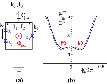
Figure 1: (Color online) (a) Current-biased flux qubit. Two current states of the three-Josephson-junction loop interact with the bias currents. $I_{0}$ is the bias current applied across the capacitance $C_{\mu\!\rm w}$, and $k_{i}$’s are the wave vectors of the Cooper pair wave function. (b) Plot for the effective potential $U_{\rm eff}(\{\phi_{\pm}\})$ with $f=0.5$ and $\phi_{-}$=0. The potential tilts due to a finite bias current $I_{0}$. The solid (dashed) line corresponds to positive (negative) $I_{0}$.

In the usual experiments for flux qubits, $\Phi^{2}_{0}/2L_{s}\sim O(10^{3}E_{J})$ is much larger than the other energy scale in the Lagrangian of Eq. (8). Hence, the last term in Eq. (9) can be removed, leaving the constraint $g(\phi_{i})=\phi_{1}+\phi_{2}+\phi_{3}-2\pi(n+f)=0$, which is the familiar flux quantization condition. The Lagrangian then has the effective potential

$$U_{\rm eff}(\{\phi_{i}\})\!=\!\!\!\sum^{3}_{i=1}E_{Ji}(1\!-\!\cos\phi_{i})\!+\!\!\frac{\Phi_{0}I_{0}}{4\pi}(\phi_{1}\!+\!\phi_{3}\!-\!\phi_{2})$$ (10)

with the constraint $g(\phi_{i})=0$. The Lagrange equation of motion with the above constraint produces the Kirchhoff equations in the qubit loop of Fig. 1(a): $I_{0}=I_{1}+I_{2}$ and $I_{1}=I_{3}$.

We introduce a coordinate transformation such as $\phi_{+}=(\phi_{2}+\phi_{3})/2$ and $\phi_{-}=(\phi_{2}-\phi_{3})/2$. In the usual flux qubit experiment, the two Josephson junctions are nearly identical; thus, we set $E_{J2}=E_{J3}=E_{J}$. Although one can treat the general case numerically, this case gives a clear and intuitive picture for our qubit system. In this case, the effective potential is given by

$$U_{\rm eff}(\{\phi_{\pm}\}) = -E_{J1}\cos(2\pi f-2\phi_{+})-2E_{J}\cos\phi_{+}\cos\phi_{-}$$ (11)

$$+\frac{\Phi_{0}I_{0}}{2\pi}(\pi f-\phi_{+}-\phi_{-}).$$

Without the last term representing the linear coupling of the phase to the external bias current $I_{0}$, the effective potential of Eq. (11) can have local minima only for $\cos\phi_{-}=\pm 1$, i.e., $\phi_{-}=j\pi$, with $j$ being an integer, where the qubit states are formed (See Fig. 2(a)).

Let the flux qubit be at the degeneracy point $f=0.5$. When there is no bias current $I_{0}=0$, $\phi_{+}\approx\pi/3(-\pi/3)$ for the counterclockwise (clockwise) current state $|\downarrow\rangle~{}(|\uparrow\rangle)$ with $\phi_{-}=0$, and the qubit energy levels corresponding to the local minima of $U_{\rm eff}(\{\phi_{\pm}\})$ are degenerate, $E_{\downarrow}=E_{\uparrow}$. In this case, the qubit is optimally biased with respect to both the current $I_{0}$ and the magnetic flux $f$. A finite bias current tilts the effective potential as shown in Fig. 2(b), where the direction of energy level tilt depends on the sign of $I_{0}$. Consequently, the effective potential of Eq. (11) is expressed as $(E_{\downarrow}-\Phi_{0}I_{0}\alpha/2\pi)|\downarrow\rangle\langle\downarrow|+(E_{\uparrow}+\Phi_{0}I_{0}\alpha/2\pi)|\uparrow\rangle\langle\uparrow|$ apart from the constant, where

$$\alpha\approx|\phi_{+}|\approx\pi/3.$$ (12)

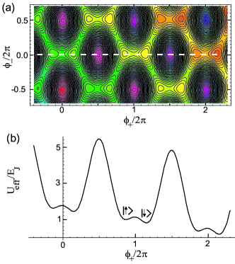
Figure 2: (Color online) (a) Effective potential of the current-biased flux qubit in the plane of $(\phi_{+},\phi_{-})$, where the effective potential of the local minima decreases as $\phi_{+}$ or $\phi_{-}$ increases. Here, we set $I_{0}/I_{\rm c}$=0.05, $f=0.5$ and $E_{J1}/E_{J}$=0.8. (b) Plot for $U_{\rm eff}(\{\phi_{\pm}\})$ along the dashed line in the upper panel.

The transitions between the two states, $|\downarrow\rangle$ and $|\uparrow\rangle$, are induced by the charging energy given by the first term of the Lagrangian in Eq. (8). Using the tight-binding approximation, we can write the Hamiltonian for our qubit system as

$${\cal H}\! = \!E_{\downarrow}|\downarrow\rangle\langle\downarrow|\!+\!E_{\uparrow}|\uparrow\rangle\langle\uparrow|-t_{q}(|\downarrow\rangle\langle\uparrow|\!+\!|\uparrow\rangle\langle\downarrow|)$$ (13)

$$-\frac{\Phi_{0}I_{0}}{2\pi}\alpha(|\downarrow\rangle\langle\downarrow|-|\uparrow\rangle\langle\uparrow|),$$

where $t_{q}$ is the transition rate between $|\downarrow\rangle$ and $|\uparrow\rangle$ states.

In order to operate the single qubit states, we apply a oscillating current,

$$I_{0}=-I_{\rm b}\sin\omega t.$$ (14)

As shown in Fig. 1(b), the effective potential vibrates with the frequency $\omega$, which produces oscillating diagonal terms in Eq. (13). In transformed coordinates, these terms appear off-diagonal, giving rise to a Rabi oscillation. The qubit states, $|0\rangle$ and $|1\rangle$, are the symmetric and the antisymmetric superpositions of $|\downarrow\rangle$ and $|\uparrow\rangle$, such that

$$|0\rangle = (|\downarrow\rangle+|\uparrow\rangle)/\sqrt{2},$$

$$|1\rangle = (|\downarrow\rangle-|\uparrow\rangle)/\sqrt{2}.$$ (15)

In the basis of $\{|0\rangle,|1\rangle\}$, the Hamiltonian is represented as

$$\tilde{\cal H}=\frac{\hbar\omega_{0}}{2}\sigma_{z}+g\sin\omega t\sigma_{x},$$ (16)

where $\hbar\omega_{0}=2t_{q}$ is the qubit frequency, and $\sigma_{x,z}$ and $I$ are the Pauli and the identity matrices, respectively. The coupling strength $g$ between the oscillating current and the qubit is given by

$$g\equiv\frac{\Phi_{0}I_{\rm b}}{2\pi}\alpha.$$ (17)

Near resonance, $\omega\approx\omega_{0}$, with a weak coupling $g/\hbar\ll\omega_{0}$, one can apply the rotating wave approximation. Jaynes Then, we can observe a Rabi oscillation between the two qubit states $|0\rangle$ and$|1\rangle$ with a Rabi frequency $\Omega_{\rm R}^{0}=g/\hbar$.

Although we do not present it explicitly, in general the number of Josephson junctions can be any odd integer larger than one. In this case, at the two sides of the qubit loop divided by the bias current line, the numbers of Josephson junctions should be different from each other so that the symmetry of the flux qubit loop is broken. Then, the resulting coupling between the current and the phase of junction enables current-driven operation of the flux qubit. For the dc-SQUID (2-junction) qubit, the bias current flows across the Josephson junctions, but the symmetry of the dc-SQUID does not allow bias-current operation of the qubit states.

III Circuit QED

The present current-biasing scheme for the flux qubit is implemented in the circuit QED architecture. In Fig. 3, the qubit is coupled to the resonator by an ac current flowing through a capacitance. The Lagrangian ${\cal L}_{r}$ of the transmission line resonator consists of the charge density mode $q(x,t)$ and the current density mode $I(x,t)$:

$${\cal L}_{r}=\int^{\frac{L}{2}}_{-\frac{L}{2}}dx\left(\frac{l}{2}I^{2}(x,t)-\frac{1}{2c}q^{2}(x,t)\right),$$ (18)

where $l$ and $c$ represent the inductance and the capacitance per unit length, and $L$ the length of the resonator. Introducing the variable $\theta(x,t)\equiv\int^{x}_{-L/2}dx^{\prime}q(x^{\prime},t)$, the Lagrangian becomes

$${\cal L}_{r}=\int^{L/2}_{-L/2}dx[(l/2)(\partial_{t}\theta)^{2}-(1/2c)(\partial_{x}\theta)^{2}],$$ (19)

where the voltage and the current of the resonator are given by $V(x,t)=\frac{1}{c}\frac{\partial\theta(x,t)}{\partial x}$ and $I(x,t)=\frac{\partial\theta(x,t)}{\partial t}$, respectively. For example, the voltage and the current of the resonator for the second harmonic mode can be represented in terms of the boson creation and annihilation operators $a^{\dagger}(t)$ and $a(t)$ as Blais

$$V(x,t) = \sqrt{\frac{\hbar\omega_{r}}{cL}}\cos\left(\frac{2\pi x}{L}\right)[a(t)+a^{\dagger}(t)],$$

$$I(x,t) = -i\sqrt{\frac{\hbar\omega_{r}}{lL}}\sin\left(\frac{2\pi x}{L}\right)[a(t)-a^{\dagger}(t)],$$ (20)

where $\omega_{r}=2\pi v/L$ and $v=\sqrt{1/lc}$. The current profile for the second harmonic mode is shown in Fig. 3.

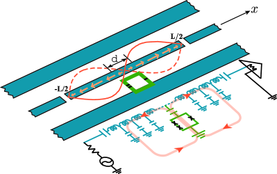
Figure 3: (Color online) Schematic diagram and equivalent lumped circuit representation of a three-junction flux qubit coupled to a transmission line resonator. The flux qubit interacts with the current mode of the resonator. The arrows in the schematic diagram and equivalent circuit show the flow of oscillating current. As shown in the equivalent circuit, the oscillating current flows between the resonator and the qubit through the capacitance. Here, $L$ is the length of the resonator, and $d$ is the width of qubit loop.

In the circuit QED scheme with superconducting charge qubit, the qubit interacts with the voltage mode $V(x,t)$. In contrast, the present current-biased flux qubit is coupled to the temporal fluctuation of local charge density, $I(x,t)$, corresponding to the bias current applied to the qubit. In Fig. 3 the resonator and the qubit are coupled by a capacitance through the region $-d/2<x<d/2$, where the charge fluctuation ${\dot{q}}(x,t)$ in the resonator produces the current flow into the qubit, $I_{0}(t)=\int^{d/2}_{-d/2}{\dot{q}}(x,t)dx.$ As a result, following the current conservation condition in the resonator, ${\dot{q}}(x,t)=\partial I(x,t)/\partial x$, and Eq. (III), the current flowing into the qubit with width $d$ is given by

$$I_{0}(t) = I(d/2,t)-I(-d/2,t)$$ (21)

$$= -2i\sqrt{\frac{\hbar\omega_{r}}{lL}}\sin\left(\frac{\pi d}{L}\right)[a(t)-a^{\dagger}(t)].$$

The interaction between the flux qubit and the bias current $I_{0}(t)$ of the resonator is given by the last term of Eq. (13). Then, from Eqs. (13) and (21), the total Hamiltonian at the degeneracy point ($E_{\downarrow}=E_{\uparrow}$) is given by

$${\cal H} = \hbar\omega_{r}\left(a^{\dagger}a+\frac{1}{2}\right)-t_{q}(|\downarrow\rangle\langle\uparrow|\!+\!|\uparrow\rangle\langle\downarrow|)$$ (22)

$$+ig(|\downarrow\rangle\langle\downarrow|-|\uparrow\rangle\langle\uparrow|)(a-a^{\dagger}),$$

where the first term comes from the oscillating mode in the resonator. The first two terms of Eq. (13) disappear at the degeneracy point. In the basis of $|0\rangle$ and $|1\rangle$, the Hamiltonian is written as

$${\tilde{\cal H}}=\hbar\omega_{r}a^{\dagger}a+\frac{\omega_{a}}{2}\sigma_{z}+ig\sigma_{x}(a-a^{\dagger}),$$ (23)

with $\hbar\omega_{a}=2t_{q}$. Here, the single qubit gate is performed by a resonant external driving microwave field Blais07 .

Since usually $d\ll L$, we have the expression of the coupling $g$ as follows:

$$g\approx\alpha\Phi_{0}\sqrt{\frac{\hbar\omega_{r}}{lL}}\left(\frac{d}{L}\right).$$ (24)

Using the usual experimental values for the parameters Abd such that $d=3~{}\mu$m, $L$=5 mm, $lL$=2.5 nH, $\omega_{r}/2\pi=$15 GHz, and $\alpha=\pi/3$, we estimate the coupling strength to be $g/h\sim 120$ MHz. For inductive coupling between the qubit and the resonator, the coupling strength, $g_{\rm IC}=\Phi I_{c}\sin\alpha$ with $\Phi$ being the magnetic flux threading the qubit due to the resonator current, can also be estimated to be

$$g_{\rm IC}\approx\frac{\mu_{0}d^{2}}{2\pi R}\sqrt{\frac{\hbar\omega_{r}}{lL}}I_{c}\sin\alpha,$$ (25)

where $R$ is the mean distance between the resonator and the qubit loop and $I_{c}=2\pi E_{J}/\Phi_{0}$. With the same parameter values, we see that $g_{\rm IC}$ is smaller than $g$ by an order of magnitude. We obtain the inductive coupling strength $g_{\rm IC}/h\sim 12$ MHz with $R=5~{}\mu$m and $E_{J}/h=200$ GHz. Note that since the qubit is located at the nodal point of the current oscillation for the second harmonic mode, the inductive coupling at this point is negligible. The above value of inductive coupling has been obtained for the first harmonic mode. We have also assumed that the capacitance density is nearly uniform along the resonator. In reality, the capacitance around the center of the resonator can be much higher due to the presence of the qubit loop, which can potentially provide a much stronger coupling $g$ in the present scheme.

IV Decoherence property

The qubit state of the present current-biased flux qubit is driven in a different way from that of the flux-driven flux qubit; thus, the decoherence property will also differ from each other. According to a recent review for the phase qubit QIP , the dephasing times of the phase qubit and the three-Josephson junction flux qubit are comparable with each other. Since the only difference between the present current-biased flux qubit and the usual current-biased dc-SQUID qubit (phase qubit) is the number of Josephson junctions in the qubit loop, the decoherence property of both qubits can be analyzed in a similar way.

In a recent experiment Steffen2 for the phase qubit, the capacitance of Josephson junction is $\sim$ 50fF while the three-Josephson junction flux qubit has a typically smaller value of capacitance of $\sim$ 3fF  Wal with a small area of the Josephson junction. For both qubits, a large shunted capacitance may reduce the decoherence from charge fluctuation. We employ the typical parameters of the three-Josephson junction flux qubit for the present current-biased qubit. Since both the capacitance and the critical current of the Josephson junction scale as the area of the junction, the critical current $I_{c}$ of junction is also much smaller.

For the present current-biased flux qubit, the dephasing due to the bias-current noise may cause decoherence of the qubit state, as in the phase qubit QIP . The current noise is related to the $1/f$ charge noise with a spectral density $S^{*}_{q}(1{\rm Hz})/f$. The phase noise is given by $\langle\phi^{2}\rangle\approx[S^{*}_{q}(1{\rm Hz})/C\Delta U](2/3)\ln(1.778\omega_{10}t)$, Nam where $C$ is the capacitance of the Josephson junction, $\Delta U$ is the barrier height of the potential, and $\omega_{10}$ is the qubit level spacing. Although for the present qubit, the spectral density $S^{*}_{q}(1{\rm Hz})$ and the capacitance $C$ are small, these contributions cancel each other in $\langle\phi^{2}\rangle$ because both the spectral density and the capacitance scale as the area of the junction Nam . Further, the qubit level spacing $\omega_{01}$ is similar between the two qubits. For the operation of the present qubit, we need not tilt the potential; thus, the barrier hight of the potential $\Delta U$ remains large. Hence, we consider the dephasing due to current noise in present qubit to still be comparable to the flux-driven flux qubit. On the other hand, the phase noise due to the critical-current fluctuation and to the flux $1/f$ fluctuations is given by $\langle\phi^{2}\rangle\approx(S^{*}_{I}(1{\rm Hz})L_{J}/\Delta U)\ln(0.401/f_{m}t)(\omega_{01}t)^{2}/6$ Nam , with the Josephson inductance $L_{J}=\Phi_{0}/2\pi I_{c}\cos\phi$ and the low-frequency cutoff $f_{m}$. For the phase noise, the argument is similar because both the spectral density $S^{*}_{I}(1{\rm Hz})$ and the critical current $I_{c}$ scale as the area of the junction.

V Summary

We propose a new circuit QED architecture for the three-Josephson-junction flux qubit, where the flux qubit is coupled to the temporal charge density fluctuations of the transmission line resonator. The flux qubit is controlled by using a bias current. When three Josephson junctions are arranged asymmetrically, the energy levels of two qubit states with different chiralities couple to the external bias current. Rabi oscillations can be induced by an ac current at an optimal point with respect to both the bias current and the external magnetic flux. Remarkably, the coupling between the qubit and the resonator is strongly enhanced compared to conventional inductive coupling.

- (1) A. Blais, R.-S. Huang, A. Wallraff, S. M. Girvin and R. J. Schoelkopf, Phys. Rev. A 69, 062320 (2004).
- (2) A. Blais, J. Gambetta, A. Wallraff, D. I. Schuster, S. M. Girvin, M. H. Devoret and R. J. Schoelkopf, Phys. Rev. A 75, 032329 (2007).
- (3) M. A. Sillapää, J. I. Park and R. W. Simmonds, Nature 449, 438 (2007).
- (4) C.-P. Yang and S. Han, Phys. Rev. A 72, 032311 (2005).
- (5) A. A. Abdumalikov, Jr., O. Astafiev, Y. Nakamura, Y. A. Pashkin and J. S. Tsai, Phys. Rev. B 78, 180502(R) (2008); J. Bourassa, J. M. Gambetta, A. A. Abdumalikov, Jr., O. Astafiev, Y. Nakamura and A. Blais, Phys. Rev. A 80, 032109 (2009).
- (6) T. Niemczyk, F. Deppe, H. Huebl, E. P. Menzel, F. Hocke, M. J. Schwarz, J. J. Garcia-Ripoll, D. Zueco, T. Hummer, E. Solano, A. Marx and R. Gross, Nature Phys. 6, 772 (2010).
- (7) A. Fedorov, A. K. Feofanov, P. Macha, P. Forn-Díaz, C. J. P. M. Harmans and J. E. Mooij, Phys. Rev. Lett. 105, 060503 (2010).
- (8) J. M. Martinis, S. Nam, J. Aumentado and C. Urbina, Phys. Rev. Lett. 89, 117901 (2002).
- (9) A. J. Berkley, H. Xu, R. C. Ramos, M. A. Gubrud, F. W. Strauch, P. R. Johnson, J. R. Anderson, A. J. Dragt, C. J. Lobb and F. C. Wellstood, Science 300, 1548 (2003).
- (10) M. Steffen, M. Ansmann, R. C. Bialczak, N. Katz, E. Lucero, R. McDermott, M. Neeley, E. M. Weig, A. N. Cleland and J. M. Martinis, Science 313, 1423 (2006).
- (11) I. Chiorescu, Y. Nakamura, C. J. P. M. Harmans and J. E. Mooij, Science 299, 1869 (2003).
- (12) A. O. Niskanen, K. Harrabi, F. Yoshihara, Y. Nakamura, S. Lloyd and J. S. Tsai, Science 316, 723 (2007).
- (13) M. Tinkham, Introduction to Superconductivity (McGraw-Hill, New York, 1996).
- (14) M. D. Kim, D. Shin and J. Hong, Phys. Rev. B 68, 134513 (2003); M. D. Kim and J. Hong, Phys. Rev. B 70, 184525 (2004).
- (15) E. T. Jaynes and F. W. Cummings, Proc. IEEE 51, 89 (1963).
- (16) J. M. Martinis, Quant. Inform. Proc. 8, 81 (2009).
- (17) M. Steffen, M. Ansmann, R. McDermott, N. Katz, R. C. Bialczak, E. Lucero, M. Neeley, E. M. Weig, A. N. Cleland and J. M. Martinis, Phys. Rev. Lett. 97, 050502 (2006).
- (18) C. H. van der Wal, A. C. J. ter Haar, F. K. Wilhelm, R. N. Schouten, C. J. P. M. Harmans, T. P. Orlando, Seth Lloyd and J. E. Mooij, Science 290, 773 (2000).
- (19) J. M. Martinis, S. Nam, J. Aumentado, K. M. Lang and C. Urbina, Phys. Rev. B 67, 094510 (2003).