The molecular systems composed of the charmed mesons in the $H\bar{S}+h.c.$ doublet

Abstract

We study the possible heavy molecular states composed of a pair of charm mesons in the H and S doublets. Since the P-wave charm-strange mesons $D_{s0}(2317)$ and $D_{s1}(2460)$ are extremely narrow, the future experimental observation of the possible heavy molecular states composed of $D_{s}/D_{s}^{\ast}$ and $D_{s0}(2317)/D_{s1}(2460)$ may be feasible if they really exist. Especially the possible $J^{PC}=1^{--}$ states may be searched for via the initial state radiation technique.

I Introduction

The new family of the charmonium or charmonium-like states include $X(3872)$, $Y(3940)$, $Y(4260)$, $Z(3930)$, $X(3940)$, $Y(4325)$, $Y(4360)$, $Y(4660)$, $Z^{+}(4430)$, $Z^{+}(4050),Z^{+}(4250)$ and $Y(4140)$ etc 2003-Choi-p262001-262001 ; 2005-Choi-p182002-182002 ; 2005-Aubert-p142001-142001 ; 2006-Uehara-p82003-82003 ; 2007-Abe-p82001-82001 ; 2007-Aubert-p212001-212001 ; 2007-Yuan-p182004-182004 ; 2007-Wang-p142002-142002 ; 2008-Choi-p142001-142001 ; 2008-Mizuk-p72004-72004 ; 2009-Aaltonen-p242002-242002 . Many states sit on the the threshold of two charmed mesons, which inspired some of them (especially those charged ones) to be candidates of heavy moleculues 2004-Swanson-p197-202 ; close1 ; 2008-Liu-p94015-94015 ; 2009-Liu-p17502-17502 ; liu1 ; liu2 ; liu3 ; liu4 ; liu5 .

In the heavy quark limit, the S-wave and P-wave heavy mesons can be categorized into three doublets: $H=(0^{-},1^{-})$, $S=(0^{+},1^{+})$, $T=(1^{+},2^{+})$. We collect their masses from PDG in Table 1. The bottom mesons in the $S$ doublet are still missing experimentally. Thus, we will adopt the theoretical predictions of the bottom meson masses in the $S$ doublet when we study the heavy flavor molecular system composed of the bottom and anti-bottom mesons.

In the framework of the meson exchange model, we have investigated the possible loosely bound molecular states composed of a pair of heavy mesons in Refs. liu1 ; liu2 ; liu3 ; liu4 ; liu5 ; liu6 . In this work, we will investigate the possible heavy molecular system constructed by the charmed and anti-charmed mesons, where one meson is in the $H$ doublet and the other one is in the $S$ doublet. In the following, we denote the heavy flavor molecular system as the $H\bar{S}+h.c.$ system for the convenience.

The $H\bar{S}+h.c.$ system can be categorized into four subsystems: $[PP_{0}^{*}]$, $[PP_{1}^{\prime}]$, $[P^{*}P_{0}^{*}]$ and $[P^{*}P_{1}^{\prime}]$. They correspond to different quantum number combinations $0^{-}+0^{+}$, $0^{-}+1^{+}$, $1^{-}+0^{+}$ and $1^{-}+1^{+}$, respectively. Since charmed mesons belong to the fundamental representation of flavor $SU(3)$, the system constructed by the charmed meson and anti-charmed meson forms an octet and a singlet: $3\otimes\bar{3}=8\oplus 1$ as illustrated in Table 2. The parameter $c=\mp 1$ in the flavor wave functions corresponds to the charge parity $C=\pm 1$ respectively for the neutral systems as pointed out in Refs. liu1 ; liu2 ; liu3 ; liu4 .

This paper is organized as follows. We review the formalism in Section II and present the results in Section III. The last section is a short summary.

II Theoretical framework

II.1 The potential model

The potential model is an effective approach to study the two-body bound state problem. For the $H\bar{S}+h.c.$ system, the scattering between the charmed and anti-charmed meson occurs via exchanging the light pseudoscalar, scalar and vector mesons, which play the role of providing long-distant, intermediate-distance and short-distance forces. At the hadron level, there exist two types of diagrams in the scattering of the charmed and anti-charmed mesons, i.e., the cross and direct diagrams as shown in Table 3. The exchanged light mesons relevant to the four subsystems $[PP_{0}^{*}]$, $[PP_{1}^{\prime}]$, $[P^{*}P_{0}^{*}]$ and $[P^{*}P_{1}^{\prime}]$ are also presented in Table 3. When writing out the scattering amplitude, the monopole form factor is introduced at every interaction vertex to compensate the off-shell effect of the exchanged light meson

$$\mathcal{F}(q)=\frac{\Lambda^{2}-m^{2}}{\Lambda^{2}-q^{2}},$$ (1)

where the phenomenological cutoff parameter $\Lambda$ is about 1 GeV. $q$ and $m$ denote the four-momentum and the mass of the exchanged meson.

$H$ doublet

charmed-up(down) meson charmed-strange meson $J^{P}$ charged mass (MeV) neutral mass (MeV) charged mass (MeV) $0^{-}$ $D^{\pm}$ 1869.3 $D^{0}$ 1864.5 $D_{s}^{\pm}$ 1968.2 $1^{-}$ $D^{*\pm}$ 2010.0 $D^{*0}$ 2006.7 $D_{s}^{*\pm}$ 2112.0 bottom-up(down) meson bottom-strange meson $J^{P}$ charged mass (MeV) neutral mass (MeV) neutral mass (MeV) $0^{-}$ $B^{\pm}$ 5279.1 $B^{0}$ 5279.5 $B_{s}^{0}$ 5365.1 $1^{-}$ $B^{*\pm}$ 5325.1 $B^{*0}$ 5325.1 $B_{s}^{*0}$ 5412.0

$S$ doublet

charmed-up(down) meson charmed-strange meson $J^{P}$ charged mass (MeV) neutral mass (MeV) charged mass (MeV) $0^{+}$ $D_{0}^{\pm}$ 2403 $D_{0}^{0}$ 2352 $D_{s0}^{\pm}$ 2317.3 $1^{+}$ $D_{1}^{\prime\pm}$ - $D_{1}^{\prime 0}$ 2427 $D_{s1}^{\prime\pm}$ 2458 bottom-up(down) meson bottom-strange meson $J^{P}$ charged mass (MeV) neutral mass (MeV) neutral mass (MeV) $0^{+}$ $B_{0}^{\pm}$ - $B_{0}^{0}$ - $B_{s0}^{0}$ - $1^{+}$ $B_{1}^{\prime\pm}$ - $B_{1}^{\prime 0}$ - $B_{s1}^{\prime 0}$ -

Table 1: The masses of the heavy mesons in the $H$ and $S$ doublets pdg .

	(a) $[PP_{0}^{*}]$ system	(b) $[PP_{1}^{\prime}]$ system
	States Wave function $[PP_{0}^{*}]^{+}$ $\frac{1}{\sqrt{2}}[D^{+}\bar{D}_{0}^{0}+c\bar{D}^{0}D_{0}^{+}]$ $[PP_{0}^{*}]^{0}$ $\frac{1}{2}[(D^{0}\bar{D}_{0}^{0}+c\bar{D}^{0}D_{0}^{0})$ $-(D^{+}D_{0}^{-}+c{D}^{-}D_{0}^{+})]$ $[PP_{0}^{*}]^{-}$ $\frac{1}{\sqrt{2}}[D^{-}\bar{D}_{0}^{0}+c\bar{D}^{0}D_{0}^{-}]$ $[PP_{0}^{*}]_{s}^{+}$ $\frac{1}{\sqrt{2}}[D_{s}^{+}\bar{D}_{0}^{0}+c\bar{D}^{0}D_{s0}^{+}]$ $[PP_{0}^{*}]_{s}^{0}$ $\frac{1}{\sqrt{2}}[D_{s}^{+}D_{0}^{-}+c{D}^{-}D_{s0}^{+}]$ $[PP_{0}^{*}]_{s}^{-}$ $\frac{1}{\sqrt{2}}[D_{s}^{-}\bar{D}_{0}^{0}+c\bar{D}^{0}D_{s0}^{-}]$ $[PP_{0}^{*}]_{\hat{s}}^{0}$ $\frac{1}{\sqrt{2}}[D^{+}D_{s0}^{-}+c{D}_{s}^{-}D_{0}^{+}]$ $[PP_{0}^{*}]_{8}^{0}$ $\frac{1}{2}[(D^{0}\bar{D}_{0}^{0}+c\bar{D}^{0}D_{0}^{0})$ $+(D^{+}D_{0}^{-}+c{D}^{-}D_{0}^{+})]$ $[PP_{0}^{*}]_{s1}^{0}$ $\frac{1}{\sqrt{2}}[D_{s}^{+}D_{s0}^{-}+cD_{s}^{-}D_{s0}^{+}]$	States Wave function $[PP_{1}^{\prime}]^{+}$ $\frac{1}{\sqrt{2}}[D^{+}\bar{D}_{1}^{\prime 0}+c\bar{D}^{0}D_{1}^{\prime+}]$ $[PP_{1}^{\prime}]^{0}$ $\frac{1}{2}[(D^{0}\bar{D}_{1}^{\prime 0}+c\bar{D}^{0}D_{1}^{\prime 0})$ $-(D^{+}D_{0}^{-}+c{D}^{-}D_{0}^{+})]$ $[PP_{1}^{\prime}]^{-}$ $\frac{1}{\sqrt{2}}[D^{-}\bar{D}_{1}^{\prime 0}+c\bar{D}^{0}D_{1}^{\prime-}]$ $[PP_{1}^{\prime}]_{s}^{+}$ $\frac{1}{\sqrt{2}}[D_{s}^{+}\bar{D}_{1}^{\prime 0}+c\bar{D}^{0}D_{s1}^{\prime+}]$ $[PP_{1}^{\prime}]_{s}^{0}$ $\frac{1}{\sqrt{2}}[D_{s}^{+}D_{1}^{\prime-}+c{D}^{-}D_{s1}^{\prime+}]$ $[PP_{1}^{\prime}]_{s}^{-}$ $\frac{1}{\sqrt{2}}[D_{s}^{-}\bar{D}_{1}^{\prime 0}+c\bar{D}^{0}D_{s1}^{\prime-}]$ $[PP_{1}^{\prime}]_{\hat{s}}^{0}$ $\frac{1}{\sqrt{2}}[D^{+}D_{s1}^{\prime-}+c{D}_{s}^{-}D_{1}^{\prime+}]$ $[PP_{1}^{\prime}]_{8}^{0}$ $\frac{1}{2}[(D^{0}\bar{D}_{1}^{\prime 0}+c\bar{D}^{0}D_{1}^{\prime 0})$ $+(D^{+}D_{1}^{\prime-}+c{D}^{-}D_{1}^{\prime+})]$ $[PP_{1}^{\prime}]_{s1}^{0}$ $\frac{1}{\sqrt{2}}[D_{s}^{+}D_{s1}^{\prime-}+cD_{s}^{-}D_{s1}^{\prime+}]$
	(c) $[P^{*}P_{0}^{*}]$ system	(d) $[P^{*}P_{1}^{\prime}]$ system
	States Wave function $[P^{*}P_{0}^{*}]^{+}$ $\frac{1}{\sqrt{2}}[D^{*+}\bar{D}_{0}^{0}+c\bar{D}^{*0}D_{0}^{+}]$ $[P^{*}P_{0}^{*}]^{0}$ $\frac{1}{2}[(D^{*0}\bar{D}_{0}^{0}+c\bar{D}^{*0}D_{0}^{0})$ $-(D^{*+}D_{0}^{-}+c{D}^{*-}D_{0}^{+})]$ $[P^{*}P_{0}^{*}]^{-}$ $\frac{1}{\sqrt{2}}[D^{*-}\bar{D}_{0}^{0}+c\bar{D}^{*0}D_{0}^{-}]$ $[P^{*}P_{0}^{*}]_{s}^{+}$ $\frac{1}{\sqrt{2}}[D_{s}^{*+}\bar{D}_{0}^{0}+c\bar{D}^{*0}D_{s0}^{+}]$ $[P^{*}P_{0}^{*}]_{s}^{0}$ $\frac{1}{\sqrt{2}}[D_{s}^{*+}D_{0}^{-}+c{D}^{*-}D_{s0}^{+}]$ $[P^{*}P_{0}^{*}]_{s}^{-}$ $\frac{1}{\sqrt{2}}[D_{s}^{*-}\bar{D}_{0}^{0}+c\bar{D}^{*0}D_{s0}^{-}]$ $[P^{*}P_{0}^{*}]_{\hat{s}}^{0}$ $\frac{1}{\sqrt{2}}[D^{*+}D_{s0}^{-}+c{D}_{s}^{*-}D_{0}^{+}]$ $[P^{*}P_{0}^{*}]_{8}^{0}$ $\frac{1}{2}[(D^{*0}\bar{D}_{0}^{0}+c\bar{D}^{*0}D_{0}^{0})$ $+(D^{*+}D_{0}^{-}+c{D}^{*-}D_{0}^{+})]$ $[P^{*}P_{0}^{*}]_{s1}^{0}$ $\frac{1}{\sqrt{2}}[D_{s}^{*+}D_{s0}^{-}+cD_{s}^{*-}D_{s0}^{+}]$	States Wave function $[P^{*}P_{1}^{\prime}]^{+}$ $\frac{1}{\sqrt{2}}[D^{*+}\bar{D}_{1}^{\prime 0}+c\bar{D}^{*0}D_{1}^{\prime+}]$ $[P^{*}P_{1}^{\prime}]^{0}$ $\frac{1}{2}[(D^{*0}\bar{D}_{1}^{\prime 0}+c\bar{D}^{*0}D_{1}^{\prime 0})$ $-(D^{*+}D_{0}^{-}+c{D}^{*-}D_{0}^{+})]$ $[P^{*}P_{1}^{\prime}]^{-}$ $\frac{1}{\sqrt{2}}[D^{*-}\bar{D}_{1}^{\prime 0}+c\bar{D}^{*0}D_{1}^{\prime-}]$ $[P^{*}P_{1}^{\prime}]_{s}^{+}$ $\frac{1}{\sqrt{2}}[D_{s}^{*+}\bar{D}_{1}^{\prime 0}+c\bar{D}^{*0}D_{s1}^{\prime+}]$ $[P^{*}P_{1}^{\prime}]_{s}^{0}$ $\frac{1}{\sqrt{2}}[D_{s}^{*+}D_{1}^{\prime-}+c{D}^{*-}D_{s1}^{\prime+}]$ $[P^{*}P_{1}^{\prime}]_{s}^{-}$ $\frac{1}{\sqrt{2}}[D_{s}^{*-}\bar{D}_{1}^{\prime 0}+c\bar{D}^{*0}D_{s1}^{\prime-}]$ $[P^{*}P_{1}^{\prime}]_{\hat{s}}^{0}$ $\frac{1}{\sqrt{2}}[D^{*+}D_{s1}^{\prime-}+c{D}_{s}^{*-}D_{1}^{\prime+}]$ $[P^{*}P_{1}^{\prime}]_{8}^{0}$ $\frac{1}{2}[(D^{*0}\bar{D}_{1}^{\prime 0}+c\bar{D}^{*0}D_{1}^{\prime 0})$ $+(D^{*+}D_{1}^{\prime-}+c{D}^{*-}D_{1}^{\prime+})]$ $[P^{*}P_{1}^{\prime}]_{s1}^{0}$ $\frac{1}{\sqrt{2}}[D_{s}^{*+}D_{s1}^{\prime-}+cD_{s}^{*-}D_{s1}^{\prime+}]$

Table 2: The flavor wave functions of the $[PP_{0}^{*}]$, $[PP_{1}^{\prime}]$, $[P^{*}P_{0}^{*}]$ and $[P^{*}P_{1}^{\prime}]$ systems. We use $[\cdots]^{a}_{b}$ to name the different states, where the superscript $a$ denotes the charge of the state and subscript $b$ is introduced to distinguish the different states in a subsystem.

According to the effective Lagrangian describing the interaction between the light and charmed mesons, one can write down the scattering amplitude between the charmed and anti-charmed mesons. Such a system can be described as

$$|J,J_{Z}\rangle=\sum_{\lambda_{1},\lambda_{2}}\langle J_{1},\lambda_{1};J_{2},\lambda_{2}|J,J_{Z}\rangle|p_{1},p_{2}\rangle,$$ (2)

where $J$ and $J_{i}$ ($i=1,2$) denote the angular momentum of the system and the componentents. The scattering amplitude $i\mathcal{M}(J,J_{Z})$ is related to the interaction potential in the momentum space in terms of the Breit approximation

$$\mathcal{V}(\mathbf{q})=-\frac{1}{\sqrt{\prod_{i}2m_{i}\prod_{f}2m_{f}}}\mathcal{M}(J,J_{Z})\;.$$ (3)

Here, $m_{i}$ and $m_{j}$ denote the masses of the initial and final statrs respectively. The potential in the coordinate space $\mathcal{V}(\mathbf{r})$ is obtained after Fourier transformation.

II.2 The effective Lagrangian

The effective Lagrangian describing the interaction between the light and heavy flavor mesons is constructed with the help of the chiral symmetry and heavy quark symmetry lag

$$\mathcal{L} = igTr[H_{b}\gamma_{\mu}\mathcal{A}^{\mu}_{ba}\gamma_{5}\bar{H}_{a}]+ig^{\prime}Tr[S_{b}\gamma_{\mu}\mathcal{A}^{\mu}_{ba}\gamma_{5}\bar{S}_{a}]+\{ihTr[S_{b}\gamma_{\mu}\mathcal{A}^{\mu}_{ba}\gamma_{5}\bar{H}_{a}]+h.c.\}$$ (4)

$$+i\beta{}Tr[H_{b}v^{\mu}(\mathcal{V}_{\mu}-\rho_{\mu})_{ba}\bar{H}_{a}]+i\lambda{}Tr[H_{b}\sigma^{\mu\nu}F_{\mu\nu}(\rho)_{ba}\bar{H}_{a}]$$

$$+i\beta{{}^{\prime}}Tr[S_{b}v^{\mu}(\mathcal{V}_{\mu}-\rho_{\mu})_{ba}\bar{S}_{a}]+i\lambda{{}^{\prime}}Tr[S_{b}\sigma^{\mu\nu}F_{\mu\nu}(\rho)_{ba}\bar{S}_{a}]$$

$$+\{i\zeta{}Tr[H_{b}\gamma^{\mu}(\mathcal{V}_{\mu}-\rho_{\mu})_{ba}\bar{S}_{a}]+i\mu{}Tr[H_{b}\sigma^{\mu\nu}F_{\mu\nu}(\rho)_{ba}\bar{S}_{a}]+h.c.\}$$

$$+g_{\sigma}{}Tr[H_{a}\sigma\bar{H}_{a}]+g^{\prime}_{\sigma}Tr[S_{a}\sigma\bar{S}_{a}]+\Big{\{}\frac{h_{\sigma}}{f_{\pi}}Tr[S_{a}(\partial_{\mu}\sigma)\gamma^{\mu}\bar{H}_{a}]+h.c.\Big{\}}.$$

The $H$ and $S$ fields, which correspond to the $(0^{-},1^{-})$ and $(0^{+},1^{+})$ doublets are defined respectively

$$H_{a} = \frac{1+v\!\!\!/}{2}[P_{a\mu}^{*}\gamma^{\mu}+iP_{a}\gamma_{5}],$$

$$\bar{H}_{b} = \gamma^{0}H^{\dagger}\gamma^{0}=[P^{*{\dagger}}_{a\mu}\gamma^{\mu}+iP_{a}^{\dagger}\gamma_{5}]\frac{1+/\!\!\!v}{2},$$

$$S_{a} = \frac{1+/\!\!\!v}{2}[P_{1a}^{\prime\mu}\gamma_{\mu}\gamma_{5}-P^{*}_{0a}],$$

$$\bar{S}_{a} = \gamma^{0}S^{\dagger}\gamma^{0}=[P^{\prime{\dagger}}_{1a\mu}\gamma^{\mu}\gamma_{5}-P^{*{\dagger}}_{0a}]\frac{1+/\!\!\!v}{2},$$ (5)

where $v=(1,0,0,0)$. Here, the annihilation operations $P,\,P^{*}_{\mu},\,P_{0}^{*},\,P_{1\mu}^{\prime}$ are of dimension $3/2$ and satisfy the normalization relations

$$\langle 0|P|Q\bar{q}(0^{-})\rangle=\sqrt{M_{H}},\qquad\langle 0|P^{*}_{\mu}|Q\bar{q}(0^{-})\rangle=\epsilon_{\mu}\sqrt{M_{H}},$$

$$\langle 0|P_{0}^{*}|Q\bar{q}(0^{+})\rangle=\sqrt{M_{S}},\qquad\langle 0|P_{1\mu}^{\prime}|Q\bar{q}(1^{+})\rangle=\epsilon_{\mu}\sqrt{M_{S}}.$$

In Eq. (4), the expansion of the axial vector gives

$$\mathcal{A}_{\mu}=\frac{1}{2}\big{(}\xi^{{\dagger}}\partial_{\mu}\xi-\xi\partial_{\mu}\xi^{{\dagger}}\big{)}=\frac{i}{f_{\pi}}\partial_{\mu}\mathcal{M}+\cdot\cdot\cdot$$ (6)

with $\xi=\exp(i\mathbb{P}/f_{\pi})$ and $f_{\pi}=132$ MeV. $\rho^{\mu}_{ba}=ig_{{}_{V}}\mathbb{V}^{\mu}_{ba}/\sqrt{2}$ and $F_{\mu\nu}(\rho)=\partial_{\mu}\rho_{\nu}-\partial_{\nu}\rho_{\mu}+[\rho_{\mu},{\ }\rho_{\nu}]$. The octet pseudoscalar and nonet vector meson matrices read as

$$\mathbb{P} = \left(\begin{array}[]{ccc}\frac{\pi^{0}}{\sqrt{2}}+\frac{\eta}{\sqrt{6}}&\pi^{+}&K^{+}\\ \pi^{-}&-\frac{\pi^{0}}{\sqrt{2}}+\frac{\eta}{\sqrt{6}}&K^{0}\\ K^{-}&\bar{K}^{0}&-\frac{2\eta}{\sqrt{6}}\end{array}\right),\quad\mathbb{V}=\left(\begin{array}[]{ccc}\frac{\rho^{0}}{\sqrt{2}}+\frac{\omega}{\sqrt{2}}&\rho^{+}&K^{*+}\\ \rho^{-}&-\frac{\rho^{0}}{\sqrt{2}}+\frac{\omega}{\sqrt{2}}&K^{*0}\\ K^{*-}&\bar{K}^{*0}&\phi\end{array}\right).$$ (13)

	Direct diagram			Crossed diagram
Subsystems	Pseudoscalar	Vector	Scalar	Pseudoscalar	Vector	Scalar
	$(\mathbb{P})$	$(\mathbb{V})$	($\mathbb{S})$	$(\mathbb{P})$	$(\mathbb{V})$	$(\mathbb{S})$
$[PP_{0}^{*}]$		$\checkmark$	$\checkmark$	$\checkmark$
$[PP_{1}^{\prime}]$		$\checkmark$	$\checkmark$		$\checkmark$	$\checkmark$
$[P^{*}P_{0}^{*}]$		$\checkmark$	$\checkmark$		$\checkmark$	$\checkmark$
$[P^{*}P_{1}^{\prime}]$	$\checkmark$	$\checkmark$	$\checkmark$	$\checkmark$	$\checkmark$	$\checkmark$

Table 3: The direct and crossed scattering diagrams with the exchanged light mesons for the $H\bar{S}+h.c.$ system .

After expanding Eq. (4), the effective Lagrangian of the pseudoscalar mesons with heavy flavor mesons reads

$$\mathcal{L}_{\mathcal{D}^{*}\mathcal{D}^{*}\mathbb{P}} = \frac{g}{f_{\pi}}\varepsilon_{\alpha\mu\beta\nu}(2iv^{\alpha}{}P^{*\mu}_{b}P^{*\nu{\dagger}}_{a})\partial^{\beta}{}\mathbb{P}_{ba},$$ (14)

$$\mathcal{L}_{\mathcal{D}^{*}\mathcal{D}\mathbb{P}} = i\frac{2g}{f_{\pi}}(P_{b}P^{*{\dagger}}_{a\lambda}-P^{*}_{b\lambda}P^{\dagger}_{a})\partial^{\lambda}{}\mathbb{P}_{ba},$$ (15)

$$\mathcal{L}_{\mathcal{D}_{1}^{\prime}\mathcal{D}_{1}^{\prime}\mathbb{P}} = \frac{g^{\prime}}{f_{\pi}}\varepsilon_{\alpha\mu\beta\nu}(2iv^{\alpha})P_{1b}^{\prime\mu}P_{1a}^{\prime\nu{\dagger}}\partial^{\beta}{}\mathbb{P}_{ba},$$ (16)

$$\mathcal{L}_{\mathcal{DD}^{*}_{0}\mathbb{P}} = \frac{h}{f_{\pi}}(2iv_{\mu})(P^{*}_{0b}P^{\dagger}_{a}-P_{b}P^{*{\dagger}}_{0a})\partial^{\mu}{}\mathbb{P}_{ba},$$ (17)

$$\mathcal{L}_{\mathcal{D}^{*}\mathcal{D}_{1}^{\prime}\mathbb{P}} = i\frac{h}{f_{\pi}}(P^{\prime}_{1b}\cdot{}P^{*{\dagger}}_{a}+P^{*}_{b}\cdot{}P^{\prime{\dagger}}_{1a})(2iv)\cdot\partial{}\mathbb{P}_{ba}\;.$$ (18)

The effective Lagrangian of the vector mesons with heavy flavor mesons reads

$$\mathcal{L}_{\mathcal{DD}\mathbb{V}} = i\frac{\beta{}g_{V}}{\sqrt{2}}P_{b}P_{a}^{\dagger}(2iv_{\mu})\mathbb{V}^{\mu}_{ba},$$ (19)

$$\mathcal{L}_{\mathcal{D}^{*}\mathcal{D}\mathbb{V}} = -2\frac{\lambda{}g_{V}}{\sqrt{2}}(2iv^{\lambda})\varepsilon_{\lambda\alpha\beta\mu}(P_{b}P^{*\mu{\dagger}}_{a}-P_{b}^{*\mu}P^{\dagger}_{a})(\partial^{\alpha}{}\mathbb{V}^{\beta})_{ba},$$ (20)

$$\mathcal{L}_{\mathcal{D}^{*}\mathcal{D}^{*}\mathbb{V}} = -i\frac{\beta{}g_{V}}{\sqrt{2}}P_{b}^{*}\cdot{}P^{*{\dagger}}_{a}(2iv\cdot{}\mathbb{V}_{ba})-i4\frac{\lambda{}g_{V}}{\sqrt{2}}P^{*\mu}_{b}P^{*\nu{\dagger}}_{a}(\partial_{\mu}{}\mathbb{V}_{\nu}-\partial_{\nu}{}\mathbb{V}_{\mu})_{ba},$$ (21)

$$\mathcal{L}_{\mathcal{D}_{0}^{*}\mathcal{D}_{0}^{*}\mathbb{V}} = -i\frac{\beta^{\prime}g_{V}}{\sqrt{2}}P^{*}_{0b}P^{*{\dagger}}_{0a}(2iv\cdot{}\mathbb{V}_{ba}),$$ (22)

$$\mathcal{L}_{\mathcal{D}_{0}^{*}\mathcal{D}^{*}\mathbb{V}} = -2\frac{\zeta{}g_{V}}{\sqrt{2}}(P_{b}^{*\mu}P^{*{\dagger}}_{0a}+P^{*}_{0b}P^{*\mu{\dagger}}_{a})\mathbb{V}_{\mu{}ba}-2\frac{\varpi g_{V}}{\sqrt{2}}(2iv^{\alpha})(P^{*\beta}_{b}P^{*{\dagger}}_{0a}-P^{*}_{0b}P^{*\beta{\dagger}}_{a})(\partial_{\alpha}{}\mathbb{V}_{\beta}-\partial_{\beta}{}\mathbb{V}_{\alpha})_{ba},$$ (23)

$$\mathcal{L}_{\mathcal{D}_{1}^{\prime}\mathcal{D}_{1}^{\prime}\mathbb{V}} = i\frac{\beta^{\prime}g_{V}}{\sqrt{2}}P^{\prime}_{1b}\cdot{}P^{\prime{\dagger}}_{1a}(2iv\cdot{}\mathbb{V}_{ba})+i4\frac{\lambda^{\prime}g_{V}}{\sqrt{2}}P^{\prime}_{1b\mu}P^{\prime{\dagger}}_{1a\nu}(\partial^{\mu}{}\mathbb{V}^{\nu}-\partial^{\nu}{}\mathbb{V}^{\mu})_{ba},$$ (24)

$$\mathcal{L}_{\mathcal{D}_{1}^{\prime}\mathcal{D}\mathbb{V}} = i2\frac{\zeta{}g_{V}}{\sqrt{2}}(P_{b}P_{1a}^{\prime\mu{\dagger}}-P^{\prime\mu}_{1b}P^{\dagger}_{a})\mathbb{V}_{\mu{}ba}+i2\frac{\varpi{}g_{V}}{\sqrt{2}}(2iv^{\alpha})(P_{b}P_{1a}^{\prime\beta{\dagger}}+P^{\prime\beta}_{1b}P^{\dagger}_{a})(\partial_{\alpha}{}\mathbb{V}_{\beta}-\partial_{\beta}{}\mathbb{V}_{\alpha})_{ba},$$ (25)

$$\mathcal{L}_{\mathcal{D}_{1}^{\prime}\mathcal{D}^{*}\mathbb{V}} = \frac{\zeta{}g_{V}}{\sqrt{2}}(2iv^{\lambda})\varepsilon_{\lambda\nu\mu\delta}(P_{b}^{*\nu}P_{1a}^{\prime\delta{\dagger}}-P_{1b}^{\prime\delta}P_{a}^{*\nu{\dagger}})\mathbb{V}^{\mu}_{ba}+2\frac{\varpi{}g_{V}}{\sqrt{2}}\varepsilon_{\nu\alpha\beta\mu}(P^{*\nu}_{b}P^{\prime\mu{\dagger}}_{1a}+P^{\prime\mu}_{1b}P^{*\nu{\dagger}}_{a})(\partial^{\alpha}{}\mathbb{V}^{\beta}-\partial^{\beta}{}\mathbb{V}^{\alpha})_{ba},$$ (26)

$$\mathcal{L}_{\mathcal{DD}_{1}^{\prime}{}\mathbb{V}} = i2\frac{\zeta{}g_{V}}{\sqrt{2}}(P_{b}P^{\prime\mu{\dagger}}_{1a}-P^{\dagger}_{a}P^{\prime\mu}_{1b})\mathbb{V}_{\mu{}ba}-i2\frac{\varpi{}g_{V}}{\sqrt{2}}(2iv^{\beta})(P_{b}P^{\prime\alpha{\dagger}}_{1a}+P^{\prime\alpha}_{1b}P^{+}_{a})(\partial_{\alpha}{}\mathbb{V}_{\beta}-\partial_{\beta}{}\mathbb{V}_{\alpha})_{ba},$$ (27)

$$\mathcal{L}_{\mathcal{D}_{1}^{\prime}\mathcal{D}_{0}^{*}\mathbb{V}} = i2\frac{\lambda^{\prime}g_{V}}{\sqrt{2}}(2iv^{\lambda})\varepsilon_{\lambda\alpha\beta\mu}(P^{*}_{0b}P^{\prime\mu{\dagger}}_{1a}+P^{\prime\mu}_{1b}P^{*{\dagger}}_{0a})(\partial^{\alpha}{}\mathbb{V}^{\beta})_{ba}\;.$$ (28)

The effective Lagrangian of the $\sigma$ meson interacting with heavy flavor mesons reads

$$\mathcal{L}_{\mathcal{DD}\sigma} = -2g_{\sigma}\sigma{}P_{b}P^{\dagger}_{b},$$ (29)

$$\mathcal{L}_{\mathcal{D}^{*}\mathcal{D}^{*}\sigma} = 2g_{\sigma}\sigma{}P^{*}_{b}\cdot{}P^{*{\dagger}}_{b},$$ (30)

$$\mathcal{L}_{\mathcal{D}_{0}^{*}\mathcal{D}_{0}^{*}\sigma} = 2g^{\prime}_{\sigma}\sigma{}P^{*}_{0b}P^{*{\dagger}}_{0b},$$ (31)

$$\mathcal{L}_{\mathcal{D}_{1}^{\prime}\mathcal{D}_{1}^{\prime}\sigma} = -2g^{\prime}_{\sigma}\sigma{}P^{\prime}_{1b}\cdot{}P^{\prime{\dagger}}_{1b},$$ (32)

$$\mathcal{L}_{\mathcal{DD}_{1}^{\prime}\sigma} = -i\frac{2h_{\sigma}}{f_{\pi}}(P^{\prime}_{1b\mu}P^{\dagger}_{b}-P_{b}P^{\prime{\dagger}}_{1b\mu})\partial^{\mu}\sigma,$$ (33)

$$\mathcal{L}_{\mathcal{D}^{*}\mathcal{D}^{*}_{0}\sigma} = -\frac{2h_{\sigma}}{f_{\pi}}(P^{*}_{0b}P^{*\lambda{\dagger}}_{b}+P^{*\lambda}_{b}P^{*{\dagger}}_{0b})\partial_{\lambda}\sigma,$$ (34)

$$\mathcal{L}_{\mathcal{D}^{*}\mathcal{D}_{1}^{\prime}\sigma} = i\frac{2h_{\sigma}}{f_{\pi}}v^{\alpha}\varepsilon_{\alpha\mu\lambda\nu}(P_{1a}^{\prime\mu}P_{a}^{*\nu{\dagger}}-P_{a}^{*\nu}P_{1a}^{\prime\mu{\dagger}})\partial^{\lambda}\sigma.$$ (35)

The values of the parameters $g^{(\prime)}$, $\beta^{(\prime)}$, $\lambda^{(\prime)}$, $h$, $\varpi$, $\zeta$, $g_{\sigma}^{(\prime)}$ and $h_{\sigma}$ are discussed in Refs. lag ; hpz .

II.3 The effective potential of the $H\bar{S}+h.c.$ system

We list the effective potentials of the states in the $H\bar{S}+h.c.$ system in Table 4. Here $V_{i}^{j}$, $Q_{i}^{j}$, $W_{i}^{j}$ and $O_{i}^{j}$ are the sub-potentials corresponding to the subsystems $[PP_{0}^{*}]$, $[PP_{1}^{\prime}]$, $[P^{*}P_{0}^{*}]$ and $[P^{*}P_{1}^{\prime}]$ respectively. The parameters in front of the sub-potentials in Table 4 are from the coefficients in the octet pseudoscalar and nonet vector meson matrices.

States	Effective potential
$[PP_{0}^{*}]^{\pm,0}$	$[-\frac{1}{2}{V}_{\rho}^{Direct}(r)+\frac{1}{2}V_{\omega}^{Direct}(r)+V_{\sigma}^{Direct}(r)]+c[-\frac{1}{2}V_{\pi}^{Cross}(r)+\frac{1}{6}V_{\eta}^{Cross}(r)]$
$[PP_{1}^{\prime}]^{\pm,0}$	$[-\frac{1}{2}Q_{\rho}^{Direct}(r)+\frac{1}{2}Q_{\omega}^{Direct}(r)+Q_{\sigma}^{Direct}(r)]+c[-\frac{1}{2}Q_{\rho}^{Cross}(r)+\frac{1}{2}Q_{\omega}^{Cross}(r)+Q_{\sigma}^{Cross}(r)]$
$[P^{*}P_{0}^{*}]^{\pm,0}$	$[-\frac{1}{2}W_{\rho}^{Direct}(r)+\frac{1}{2}W_{\omega}^{Direct}(r)+W_{\sigma}^{Direct}(\sigma)]+c[-\frac{1}{2}W_{\rho}^{Cross}(r)+\frac{1}{2}W_{\omega}^{Cross}(r)+W_{\sigma}^{Cross}(r)]$
$[P^{*}P_{1}^{\prime}]^{\pm,0}$	$[-\frac{1}{2}O_{\rho}^{Direct}(r)+\frac{1}{2}O_{\omega}^{Direct}(r)-\frac{1}{2}O_{\pi}^{Direct}(r)+\frac{1}{6}O_{\eta}^{Direct}(r)+O_{\sigma}^{Direct}(r)]$
	$+c[-\frac{1}{2}O_{\pi}^{Cross}(r)+\frac{1}{6}O_{\eta}^{Cross}(r)-\frac{1}{2}O_{\rho}^{Cross}(r)+\frac{1}{2}O_{\omega}^{Cross}(r)+O_{\sigma}^{Cross}(r)]$
$[PP_{0}^{*}]_{s}^{\pm,0},[PP_{0}^{*}]_{\hat{s}}^{0}$	$c[-\frac{1}{3}V_{\eta}^{Cross}(r)]$
$[PP_{1}^{\prime}]_{s}^{\pm,0},[PP_{1}^{\prime}]_{\hat{s}}^{0}$	0
$[P^{*}P_{0}^{*}]_{s}^{\pm,0},[P^{*}P_{0}^{*}]_{\hat{s}}^{0}$	0
$[P^{*}P_{1}^{\prime}]_{s}^{\pm,0},[P^{*}P_{1}^{\prime}]_{\hat{s}}^{0}$	$[-\frac{1}{3}O_{\eta}^{Direct}(r)]+c[-\frac{1}{3}O_{\eta}^{Cross}(r)]$
$[PP_{0}^{*}]_{s1}^{0}$	$[V_{\phi}^{Direct}(r)]+c[\frac{2}{3}V_{\eta}^{Cross}(r)]$
$[PP_{1}^{\prime}]_{s1}^{0}$	$[Q_{\phi}^{Direct}(r)]+c[Q_{\phi}^{Cross}(r)]$
$[P^{*}P_{0}^{*}]_{s1}^{0}$	$[W_{\phi}^{Direct}(r)]+c[W_{\phi}^{Cross}(r)]$
$[P^{*}P_{1}^{\prime}]_{s1}^{0}$	$[O_{\phi}^{Direct}(r)+\frac{2}{3}O_{\eta}^{Direct}(r)]+c[O_{\phi}^{Cross}(r)+\frac{2}{3}O_{\eta}^{Cross}(r)]$
$[PP_{0}^{*}]_{8}^{0}$	$[\frac{3}{2}V_{\rho}^{Direct}(r)+\frac{1}{2}V_{\omega}^{Direct}(r)+V_{\sigma}^{Direct}(r)]+c[\frac{3}{2}V_{\pi}^{Cross}(r)+\frac{1}{6}V_{\eta}^{Cross}(r)]$
$[PP_{1}^{\prime}]_{8}^{0}$	$[\frac{3}{2}Q_{\rho}^{Direct}(r)+\frac{1}{2}Q_{\omega}^{Direct}(r)+Q_{\sigma}^{Direct}(r)]+c[\frac{3}{2}Q_{\rho}^{Cross}(r)+\frac{1}{2}Q_{\omega}^{Cross}(r)+Q_{\sigma}^{Cross}(r)]$
$[P^{*}P_{0}^{*}]_{8}^{0}$	$[\frac{3}{2}W_{\rho}^{Direct}(r)+\frac{1}{2}W_{\omega}^{Direct}(r)+W_{\sigma}^{Direct}(r)]+c[\frac{3}{2}W_{\rho}^{Cross}(r)+\frac{1}{2}W_{\omega}^{Cross}(r)+W_{\sigma}^{Cross}(r)]$
$[P^{*}P_{1}^{\prime}]_{8}^{0}$	$[\frac{3}{2}O_{\rho}^{Direct}(r)+\frac{1}{2}O_{\omega}^{Direct}(r)+\frac{3}{2}O_{\pi}^{Direct}(r)+\frac{1}{6}O_{\eta}^{Direct}(r)+O_{\sigma}^{Direct}(r)]$
	$+c[\frac{3}{2}O_{\pi}^{Cross}(r)+\frac{1}{6}O_{\eta}^{Cross}(r)+\frac{3}{2}O_{\rho}^{Cross}(r)+\frac{1}{2}O_{\omega}^{Cross}(r)+O_{\sigma}^{Cross}(r)]$

Table 4: The total effective potentials of the states in the subsystems $[PP_{0}^{*}]$, $[PP_{1}^{\prime}]$, $[P^{*}P_{0}^{*}]$ and $[P^{*}P_{1}^{\prime}]$.

For the $[P{P}_{0}^{*}]$ subsystem, the sub-potentials are

$$V^{Direct}_{\mathbb{V}}(r) = -\frac{1}{2}\beta\beta^{\prime}g_{V}^{2}Y(\Lambda,q_{0},m_{\mathbb{V}},r),$$ (36)

$$V^{Direct}_{\sigma}(r) = -g_{\sigma}g_{\sigma}^{\prime}Y(\Lambda,q_{0},m_{\sigma},r),$$ (37)

$$V^{Cross}_{\mathbb{P}}(r) = \frac{h^{2}{q_{0}^{\prime}}^{2}}{f_{\pi}^{2}}Y(\Lambda,q_{0}^{\prime},m_{\mathbb{P}},r).$$ (38)

For the $[P{P}_{1}^{\prime}]$ subsystem, the sub-potentials are

$$Q^{Direct}_{\mathbb{V}}(r) = -\frac{1}{2}\beta\beta^{\prime}g_{V}^{2}Y(\Lambda,q_{0},m_{\mathbb{V}},r),$$ (39)

$$Q^{Direct}_{\sigma}(r) = -g_{\sigma}g_{\sigma}^{\prime}Y(\Lambda,q_{0},m_{\sigma},r),$$ (40)

$$Q^{Cross}_{\mathbb{V}}(r) = -\frac{g_{V}^{2}}{4}(2\zeta^{2}-8\zeta\varpi q_{0}^{\prime}+8\varpi^{2}{q_{0}^{\prime}}^{2})Y(\Lambda,q_{0}^{\prime},m_{\mathbb{V}},r)$$ (41)

$$+\frac{g_{V}^{2}}{12}(8\mu^{2}-\frac{2\zeta^{2}}{m_{V}^{2}})Z(\Lambda,q_{0}^{\prime},m_{\mathbb{V}},r),$$

$$Q^{Cross}_{\sigma}(r) = -\frac{h_{\sigma}^{2}}{3f_{\pi}^{2}}Z(\Lambda,q_{0}^{\prime},m_{\sigma},r).$$ (42)

The sub-potentials relevant to the $[P^{*}{P}_{0}^{*}]$ subsystem are

$$W^{Direct}_{\mathbb{V}}(r) = -\frac{1}{2}\beta\beta^{\prime}g_{V}^{2}Y(\Lambda,q_{0},m_{\mathbb{V}},r),$$ (43)

$$W^{Direct}_{\sigma}(r) = -g_{\sigma}g_{\sigma}^{\prime}Y(\Lambda,q_{0},m_{\sigma},r),$$ (44)

$$W^{Cross}_{\mathbb{V}}(r) = \frac{1}{4}g_{V}^{2}(2\zeta^{2}-8\zeta\varpi q_{0}^{\prime}+8\varpi^{2}{q_{0}^{\prime}}^{2})Y(\Lambda,q_{0}^{\prime},m_{\mathbb{V}},r)$$ (45)

$$-\frac{1}{12}g_{V}^{2}(8\mu^{2}-\frac{2\zeta^{2}}{m_{\mathbb{V}}^{2}})Z(\Lambda,q_{0}^{\prime},m_{\mathbb{V}},r),$$

$$W^{Cross}_{\sigma}(r) = \frac{h_{\sigma}^{2}}{f_{\pi}^{2}}\frac{1}{3}Z(\Lambda,q_{0}^{\prime},m_{\sigma},r).$$ (46)

For the $[P^{*}\bar{P}_{1}^{\prime}]$ subsystem, the relevant potentials are

$$O^{Direct}_{\mathbb{V}}(r) = -\frac{1}{2}g_{V}^{2}\beta\beta^{\prime}C[J]Y(\Lambda,q_{0},m_{\mathbb{V}},r)-2g_{V}^{2}\lambda\lambda^{\prime}B[J]Z(\Lambda,q_{0},m_{V},r),$$ (47)

$$O^{Direct}_{\mathbb{P}}(r) = -\frac{gg^{\prime}}{f_{\pi}^{2}}A[J]Z(\Lambda,q_{0},m_{\mathbb{V}},r),$$ (48)

$$O^{Direct}_{\sigma}(r) = -g_{\sigma}g_{\sigma}^{\prime}C[J]Y(\Lambda,q_{0},m_{\mathbb{V}},r),$$ (49)

$$O^{Cross}_{\mathbb{V}}(r) = \frac{1}{4}g_{V}^{2}(2\zeta^{2}-8\zeta\varpi q_{0}^{\prime}+8\varpi^{2}{q_{0}^{\prime}}^{2})C[J]Y(\Lambda,q_{0}^{\prime},m_{\mathbb{V}},r)$$ (50)

$$-\frac{1}{4}g_{V}^{2}(\frac{2\zeta^{2}}{m_{\mathbb{V}}^{2}}-8\mu^{2})A[J]Z(\Lambda,q_{0},m_{\mathbb{V}},r),$$

$$O^{cross}_{\mathbb{P}}(r) = -\frac{h^{2}}{f_{\pi}^{2}}{q_{0}^{\prime}}^{2}C[J]Y(\Lambda,q_{0}^{\prime},m_{\mathbb{P}},r),$$ (51)

$$O^{Cross}_{\sigma}(r) = -\frac{h_{\sigma}^{2}}{f_{\pi}^{2}}A[J]Z(\Lambda,q_{0}^{\prime},m_{\sigma},r)$$ (52)

with the coefficients $A[J]$, $B[J]$ and $C[J]$

$$\begin{array}[]{|c|c|c|c|}\hline\cr\hline\cr&$J=0$&$J=1$&$J=2$\\ \hline\cr$A[J]$&2/3&1/3&-1/3\\ $B[J]$&4/3&2/3&-2/3\\ $C[J]$&1&1&1\\ \hline\cr\hline\cr\end{array}\,.$$ (57)

In the above expressions, the functions $Y(\Lambda,\kappa,m,r)$ and $Z(\Lambda,\kappa,m,r)$ are defined as

$$Y(\Lambda,\kappa,m,r) = \int\frac{d^{3}q}{(2\pi)^{3}}e^{i\mathbf{q}\cdot\mathbf{r}}\frac{1}{\mathbf{q}^{2}-\kappa^{2}-m^{2}}\bigg{(}\frac{\Lambda^{2}-m^{2}}{\Lambda^{2}-\mathbf{q}^{2}+\kappa^{2}}\bigg{)}^{2}$$ (58)

$$= \left\{\begin{array}[]{ll}\mbox{if $|\kappa|\leq m$},\quad-\frac{1}{4\pi r}\left(e^{-\zeta_{1}r}-e^{-\zeta_{2}r}\right)+\frac{1}{8\pi}\left(\zeta_{2}-\frac{\zeta_{1}^{2}}{\zeta_{2}}\right)e^{-\zeta_{2}r}&\\ \mbox{otherwise},\quad-\frac{1}{4\pi r}\left(\cos(\zeta_{1}^{\prime}r)-e^{-\zeta_{2}r}\right)+\frac{1}{8\pi}\left(\zeta_{2}+\frac{\zeta_{1}^{\prime 2}}{\zeta_{2}}\right)e^{-\zeta_{2}r}&\end{array}\right.$$ (61)

and

$$Z(\Lambda,\kappa,m,r) = -\frac{1}{r^{2}}\frac{\partial}{\partial r}\left(r^{2}\frac{\partial}{\partial r}Y(\Lambda,\kappa,m,r)\right),$$ (62)

where $\zeta_{1}=\sqrt{m^{2}-\kappa^{2}}$, $\zeta_{1}^{\prime}=\sqrt{\kappa^{2}-m^{2}}$, and $\zeta_{2}=\sqrt{\Lambda^{2}-\kappa^{2}}$. We take $q_{0}=0$ and the mass differences $q_{0}^{\prime}$ as $(m_{P_{0}}-m_{P})$, $(m_{P^{\prime}_{1}}-m_{P})$, $(m_{P_{0}}-m_{P^{*}})$ and $(m_{P_{1}^{\prime}}-m_{P^{*}})$ corresponding to the $[PP_{0}^{*}]$, $[PP_{1}^{\prime}]$, $[P^{*}P_{0}^{*}]$ and $[P^{*}P_{1}^{\prime}]$ subsystems respectively.

III Numerical results

In the following, we present the numerical results for the different systems. Throughout this work, $\mu$ denotes the reduced mass of the corresponding system in all figures of the numerical results.

III.1 The $[PP_{0}^{*}]$ system

III.1.1 $[PP_{0}^{*}]^{\pm,0}$

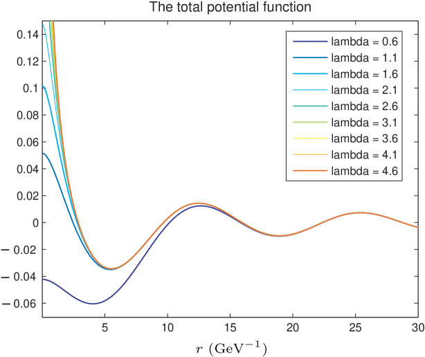
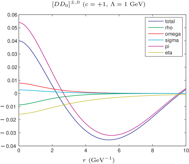
(a)	(b)
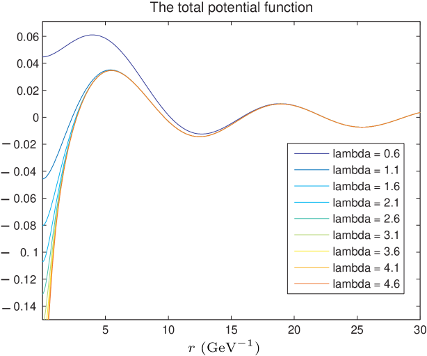
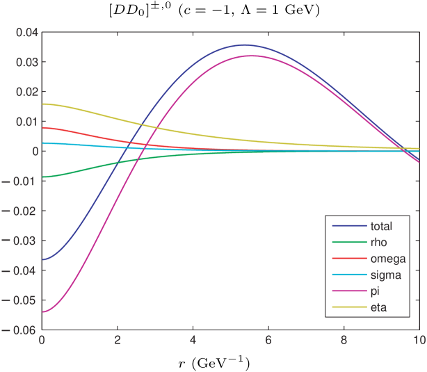
(c)	(d)

Figure 1: (a) The variation of the total potential of the $[DD_{0}]^{\pm,0}$ system $(c=+1)$ with $r$ and $\Lambda$; (b) the exchange potentials of the $\pi,\,\eta,\,\sigma,\,\rho,\,\omega$ mesons of the $[DD_{0}]^{\pm,0}$ system $(c=+1)$ with $\Lambda=1$ GeV; (c) the variation of the total potential of the $[DD_{0}]^{\pm,0}$ system $(c=-1)$ with $r$ and $\Lambda$; (d) the exchange potentials of the $\pi,\,\eta,\,\sigma,\,\rho,\,\omega$ mesons of the $[DD_{0}]^{\pm,0}$ system $(c=-1)$ with $\Lambda=1$ GeV. The above potentials are obtained when $g_{\sigma}g_{\sigma}^{\prime}>0$ and $\beta\beta^{\prime}>0$. Here, $|h|=0.56$, $|g_{\sigma}|=0.76$, $|g_{\sigma}^{\prime}|=0.76$, $|\beta|=0.909$ and $|\beta^{\prime}|=0.533$.

The total potentials of the $[PP_{0}^{*}]^{\pm,0}$ system with $c=\pm 1$ and the typical values of $\Lambda$ are presented in Fig. 1. The comparison of the total potential with the partial potentials indicates that the $\pi$ exchange plays the dominant role in the total effective potential of the $[PP_{0}^{*}]^{\pm,0}$ system with $c=\pm 1$. Here we only illustrate the potential with $\Lambda=1$ GeV in Fig. 1 (b) and (d).

Since the one $\pi$ exchange potential is dominant in the total potential of $[PP_{0}^{*}]^{\pm,0}$, it’s enough to consider the one $\pi$ exchange force only when we study the bound state solution of the $[PP_{0}^{*}]^{\pm,0}$ system. The one $\pi$ exchange potential is proportional to the coupling constant $h$. Thus, we try to solve the schrödinger equation with the obtained one pion exchange potential under some typical values of $h$.

For the $[PP_{0}^{*}]^{\pm,0}$ system with $c=+1$, we can find the bound state solutions numerically. As shown in Fig. 2, the binding energy $E_{0}$ decreases when $\Lambda$ becomes larger. One may further check the corresponding wave function to make sure whether the bound state solution is reasonable. An example is shown in Fig. 2 (a) with $h\equiv-0.56$. As $\Lambda$ increases, the wave function oscillates at large distance. In other words, smaller $\Lambda$ values such as $\Lambda<0.75$ GeV lead to the bound state wave function with less oscillating behavior. On the other hand, the reasonable range of $\Lambda$ is sometimes assumed to be around $1$ GeV.

Enhancing the coupling constant helps to form the bound state of $[PP_{0}^{*}]^{\pm,0}$ system with $c=+1$. For example, there exist a very reasonable bound state solution with $1.3h$ corresponding to a shallow binding energy, a reasonable $\Lambda$ and wave function with good behavior as shown in Fig. 2 (b). If the coupling constant becomes even larger, the binding energy of the $[PP_{0}^{*}]^{\pm,0}$ system with $c=+1$ becomes deeper. As shown in Fig 2 (c) and (d), there only exist deeply bound states for the $[PP_{0}^{*}]^{\pm,0}$ system ($c=+1$) with $2h$ and $3h$.

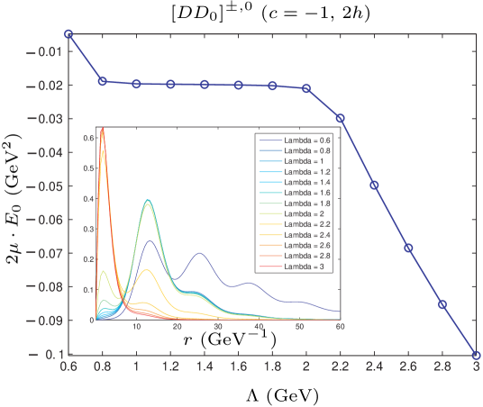
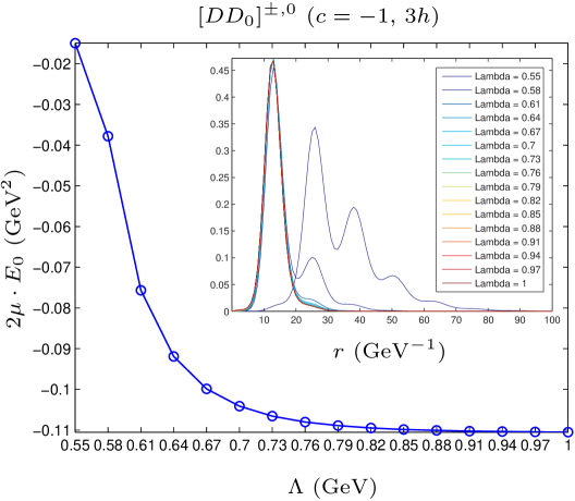
(a)	(b)

Figure 3: The dependence of the binding energy of $[DD_{0}]^{\pm,0}$ system $(c=-1)$ on $\Lambda$ and the wave function of this system. Here, we only consider the single $\pi$ exchange potential. (a) and (b) correspond to the case of $2h$ and $3h$ with $|h|=0.56$ respectively. When taking $1h$, we can not find the bound state solution.

For the $[PP_{0}^{*}]^{\pm,0}$ system with $c=-1$, we can not find the bound state solution with $1h$. With $2h$ and $\Lambda=2.6\sim 3$ GeV, the wave function of the $[PP_{0}^{*}]^{\pm,0}$ system with $c=-1$ becomes non-oscillating. When further increasing the coupling constant to $3h$, there exists a $[PP_{0}^{*}]^{\pm,0}$ bound state with $c=-1$ and $\Lambda$ near 1 GeV. The numerical results of the $[PP_{0}^{*}]^{\pm,0}$ system with $c=-1$ are presented in Fig. 3.

III.1.2 $[PP_{0}^{*}]_{s}^{\pm,0},\,[PP_{0}^{*}]_{\hat{s}}^{0}$

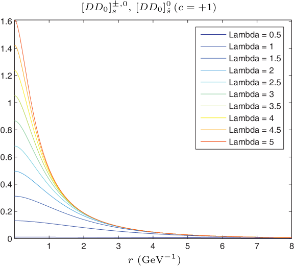
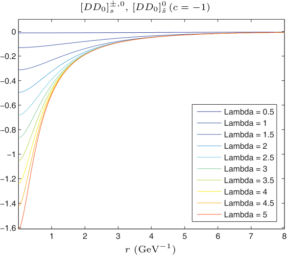
(a)	(b)

Figure 4: (a) The variation of the total potential of the $[DD_{0}]_{s}^{\pm,0},[DD_{0}]_{\hat{s}}^{0}$ system $(c=+1)$ with $r$ and $\Lambda$; (b) The variation of the total potential of the $[DD_{0}]_{s}^{\pm,0},[DD_{0}]_{\hat{s}}^{0}$ system $(c=-1)$ with $r$ and $\Lambda$. Here, we take $|h|=0.56$.

The potential of $[PP_{0}^{*}]_{s}^{\pm,0},\,[PP_{0}^{*}]_{\hat{s}}^{0}$ is shown in Fig. 4, where only the $\eta$ meson exchange contributes. The effective potential is repulsive and attractive for $c=+1$ and $c=-1$ respectively. There does not exist any bound states with $c=+1$.

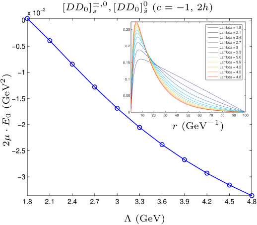
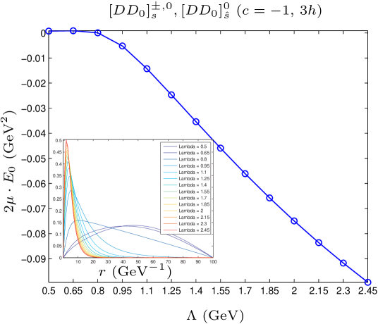
(a)	(b)

Figure 5: The dependence of the binding energy of the $[DD_{0}]_{s}^{\pm,0},[DD_{0}]_{\hat{s}}^{0}$ system $(c=-1)$ on $\Lambda$ and the wave function of this system. Here, we only consider the single $\eta$ exchange potential. (a) and (b) correspond to the case of $2h$ and $3h$ with $|h|=0.56$ respectively. When taking $1h$, we can not find the bound state solution.

For the $[PP_{0}^{*}]_{s}^{\pm,0},\,[PP_{0}^{*}]_{\hat{s}}^{0}$ system with $c=-1$, we can not find the bound state solution with $h\equiv-0.56$. We illustrate the numerical results with $2h$ and $3h$ in Fig. 5. There may exist a $[PP_{0}^{*}]_{s}^{\pm,0},\,[PP_{0}^{*}]_{\hat{s}}^{0}$ bound state with $c=-1$ if the coupling constant is around several $h$.

III.1.3 $[PP_{0}^{*}]_{s1}^{0}$

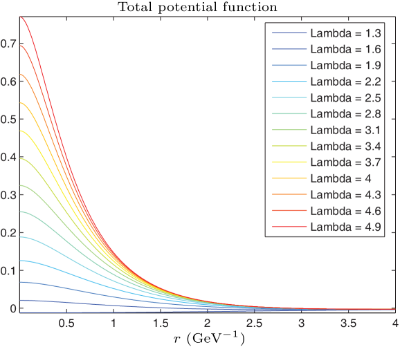
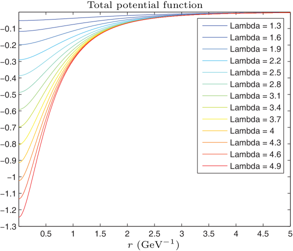
(a)	(b)
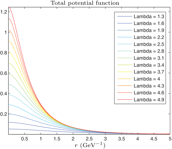
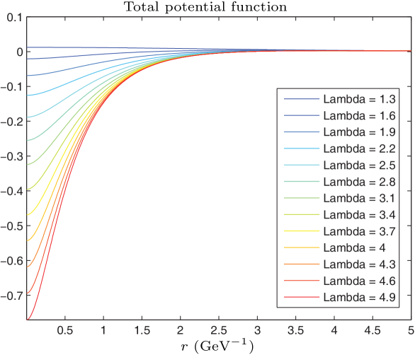
(c)	(d)
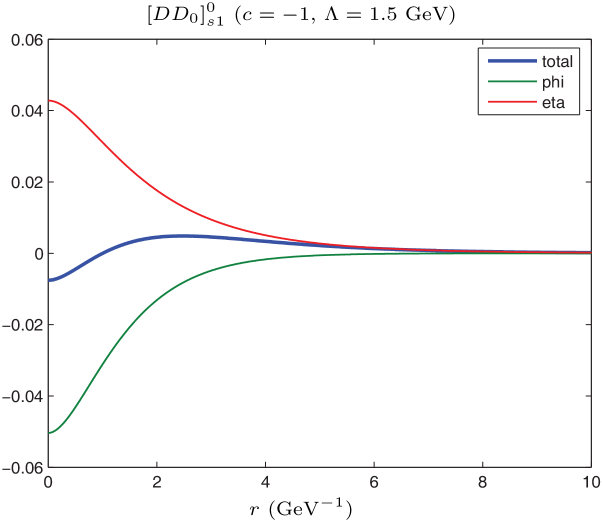
(e)	(f)

Figure 6: (a), (b), (c) and (d) are the total potentials of the $[DD_{0}]_{s1}^{0}$ systems with $(c=+1,\,\beta\beta^{\prime}>0)$, $(c=+1,\,\beta\beta^{\prime}<0)$, $(c=-1,\,\beta\beta^{\prime}>0)$ and $(c=-1,\,\beta\beta^{\prime}<0)$ respectively. Under taking $\Lambda=1.5$ GeV, (e) and (f) are the partial potentials of the $[DD_{0}]_{s1}^{0}$ system with $(c=+1,\,\beta\beta^{\prime}<0)$ and $(c=-1,\,\beta\beta^{\prime}<0)$ respectively. Here, we take $|h|=0.56$, $|\beta|=0.909$ and $|\beta^{\prime}|=0.533$.

In Fig. 6, we plot the variation of the effective potential of the $[PP_{0}^{*}]_{s1}^{0}$ system with $r$ and different coupling constants and the cutoff parameter. The $\eta$ and $\phi$ meson exchange contributes to the total effective potential. The cutoff $\Lambda$ should be larger than the mass of $\phi$ meson. The total effective potentials with $(c=+1,\beta\beta^{\prime}<0)$ and $(c=-1,\beta\beta^{\prime}<0)$ are attractive while the effective potentials with $(c=+1,\beta\beta^{\prime}>0)$ and $(c=-1,\beta\beta^{\prime}>0)$ are repulsive. The comparison of the total potential with the $\eta$ and $\phi$ meson exchange potential is given in Fig. 6 (e) and (f) with $\Lambda=1.5$ GeV.

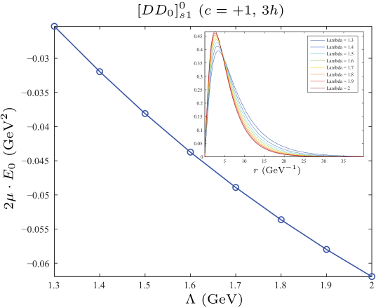
(a)	(b)
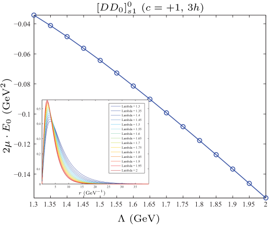
(c)

Figure 7: The dependence of the binding energy of the $[DD_{0}]_{s1}^{0}$ system $(c=+1)$ on $\Lambda$ and the wave function of this system. Here, we consider the contribution of the $\eta$ and $\phi$ exchange potentials. (a) is for $(c=+1,\,\beta\beta^{\prime}>0)$; (b) and (c) are for $(c=+1,\,\beta\beta^{\prime}<0)$. When taking $(c=-1,\,\beta\beta^{\prime}<0)$, we can not find the bound state solution. Here, we take $|h|=0.56$, $|\beta|=0.909$ and $|\beta^{\prime}|=0.533$.

For the $[PP_{0}^{*}]_{s1}^{0}$ system with $c=-1$, there does not exist a bound state not only for the case $\beta\beta^{\prime}>0$ but also for $\beta\beta^{\prime}<0$. For the $[PP_{0}^{*}]_{s1}^{0}$ system with $c=+1$ and $\beta\beta^{\prime}>0$, a reasonable solution of bound state appears with $3h$. For the $[PP_{0}^{*}]_{s1}^{0}$ system with $c=+1$ and $\beta\beta^{\prime}<0$, there does not exist a bound state with $1h$. The bound state solution appears with $2h$ and $3h$. The detailed numerical results of the $[PP_{0}^{*}]_{s1}^{0}$ system with $c=+1$ are shown in Fig. 7.

III.1.4 $[PP_{0}^{*}]_{8}^{0}$

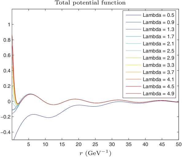
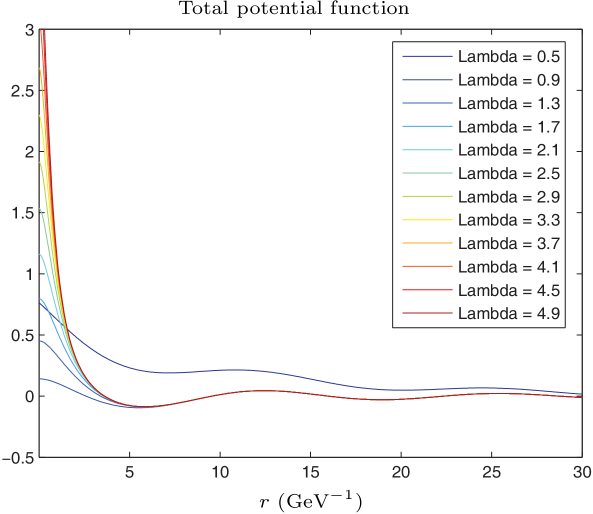
(a)	(b)
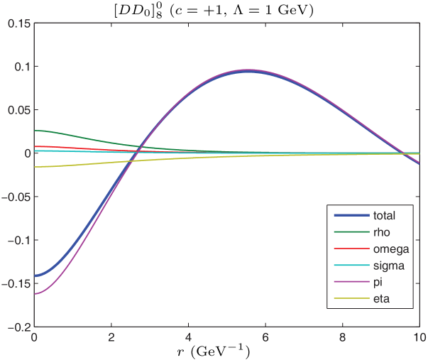
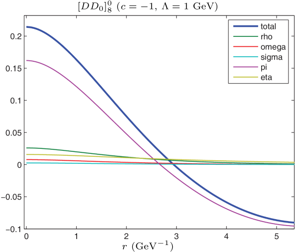
(c)	(d)

Figure 8: (a) and (b) are the total potentials of the $[DD_{0}]_{8}^{0}$ systems with $c=+1$ and $c=-1$ respectively. With $\Lambda=1$ GeV, diagrams (c) and (d) illustrate the partial potentials of the $[DD_{0}]_{8}^{0}$ system with $c=+1$ and $c=-1$ respectively. The above potentials are obtained with $g_{\sigma}g_{\sigma}^{\prime}>0$ and $\beta\beta^{\prime}>0$. Here, $|h|=0.56$, $|g_{\sigma}|=0.76$, $|g_{\sigma}^{\prime}|=0.76$, $|\beta|=0.909$ and $|\beta^{\prime}|=0.533$.

The dependence of the total potential of the $[PP_{0}^{*}]_{8}^{0}$ system on $\Lambda$ is presented in Fig. 8. The total effective potential oscillates with $r$. The $\pi$, $\eta$, $\sigma$, $\rho$ and $\omega$ exchange contributes to the total exchange potential. With $\Lambda=1$ GeV, the corresponding $\pi$, $\eta$, $\sigma$, $\rho$ and $\omega$ exchange potentials for the $[PP_{0}^{*}]_{8}^{0}$ systems with $c=\pm 1$ are given in 8 (c) and (d). The $\pi$ exchange potential is dominant. Therefore, we only consider the single pion exchange potential when we explore whether there exists the bound state solution of the $[PP_{0}^{*}]_{8}^{0}$ system.

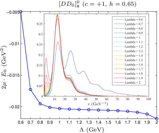
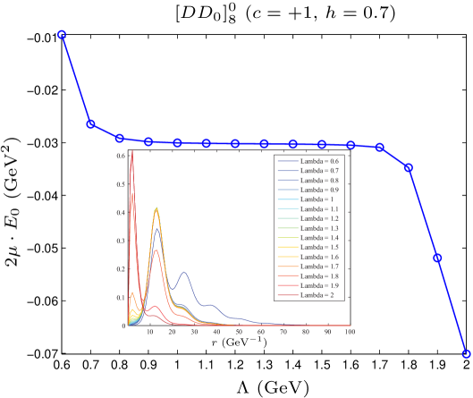
(a)	(b)
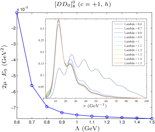
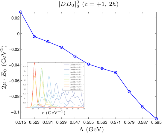
(c)	(d)
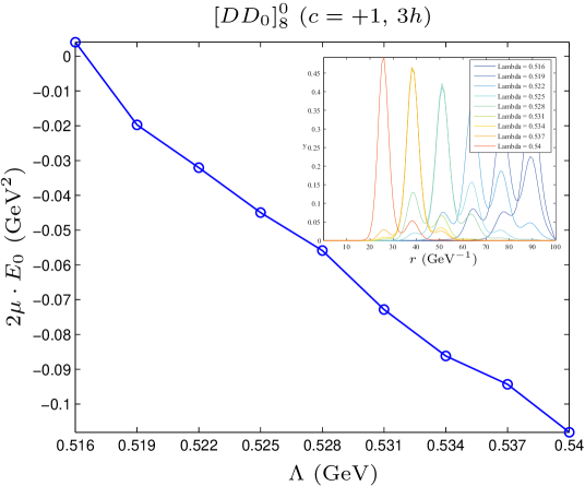
(e)

Figure 9: The dependence of the binding energy of the $[DD_{0}]_{8}^{0}$ system $(c=+1)$ on $\Lambda$ and the wave function of this system. Here, we only consider the contribution of the $\pi$ exchange potentials. We take different values of $h$, in diagrams (a)-(e). The absolute value of $h$ in $1h,\,2h,\,3h$ is 0.56.

For the $[PP_{0}^{*}]_{8}^{0}$ system with $c=+1$, there exists a bound state solution. The variation of the binding energy of $[PP_{0}^{*}]_{8}^{0}$ with $c=+1$ is shown in Fig. 9 with different values of the coupling constant. The wave functions is not reasonable when taking $|h|=0.56,\,0.65,\,0.7$, which corresponds to the shallow binding energy of the $[PP_{0}^{*}]_{8}^{0}$ system with $c=+1$. Increasing the coupling constant to $2h$ leads to a bound state solution with a reasonable wave function.

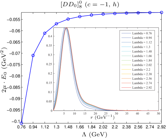
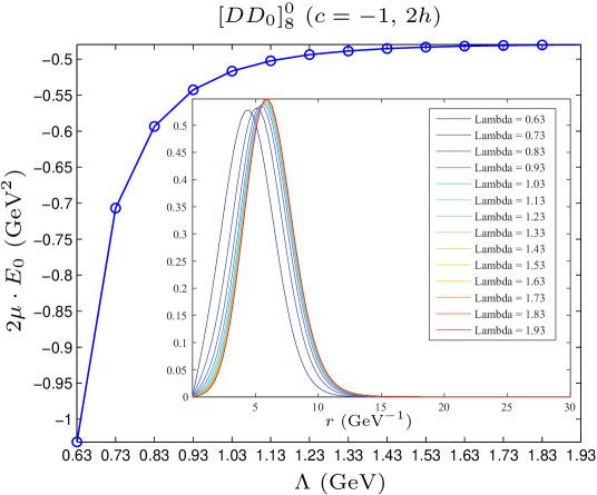
(a)	(b)

Figure 10: The binding energy of the $[DD_{0}]_{8}^{0}$ system $(c=-1)$ and the wave function of this system. Here, we only consider the $\pi$ exchange potential with $1h,\,2h$ in diagrams (a)-(c) respectively. Here, $|h|=0.56$.

The numerical result presented in Fig. 10 shows that there exists a $[PP_{0}^{*}]_{8}^{0}$ bound state with $c=-1$.

III.2 The $[PP_{1}^{\prime}]$ system

III.2.1 $[PP_{1}^{\prime}]^{\pm,0}$

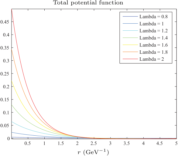
(a)	(b)
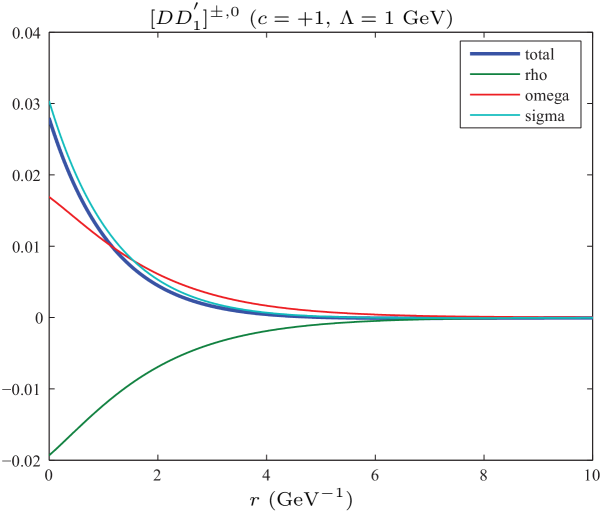
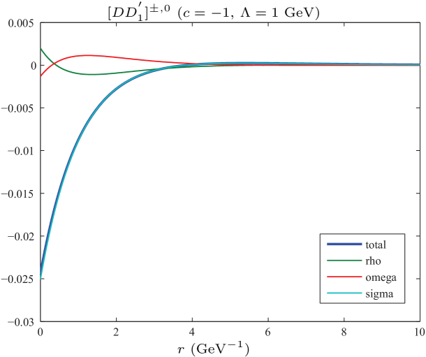
(c)	(d)

Figure 11: (a) The variation of the total potential of the $[DD_{1}^{\prime}]^{\pm,0}$ system $(c=+1)$ with $r$ and $\Lambda$; (b) the variation of the total potential of the $[DD_{1}^{\prime}]^{\pm,0}$ system $(c=-1)$ with $r$ and $\Lambda$; (c) the exchange potentials of the $\sigma,\,\rho,\,\omega$ mesons of the $[DD_{1}^{\prime}]^{\pm,0}$ system $(c=+1)$ with $\Lambda=1$ GeV; (d) the exchange potentials of the $\sigma,\,\rho,\,\omega$ mesons of the $[DD_{1}^{\prime}]^{\pm,0}$ system $(c=-1)$ with $\Lambda=1$ GeV. The above potentials are obtained with $g_{\sigma}g_{\sigma}^{\prime}>0$, $\beta\beta^{\prime}>0$ and $\zeta\varpi>0$. Here, $|g_{\sigma}|=0.76$, $|g_{\sigma}^{\prime}|=0.76$, $|h_{\sigma}|=0.323$, $|\beta|=0.909$ and $|\beta^{\prime}|=0.533$, $\zeta=0.727$ and $\varpi=0.364$.

The $\sigma$, $\rho$ and $\omega$ meson exchange contributes to the total effective potential of the $[PP_{1}^{\prime}]^{\pm,0}$ system. Since the $\rho$ and $\omega$ exchange potentials cancel each other, the $\sigma$ meson exchange potential is dominant. We only need to consider the $\sigma$ exchange potential in order to explore whether there exists a $[PP_{1}^{\prime}]^{\pm,0}$ bound state. In Fig. 11, the effective potential of the $[PP_{1}^{\prime}]^{\pm,0}$ system is presented. The $\sigma$ exchange potential of the $[PP_{1}^{\prime}]^{\pm,0}$ system with $c=+1$ is repulsive. There does not exist a $[PP_{1}^{\prime}]^{\pm,0}$ bound state with $c=+1$.

For the $[PP_{1}^{\prime}]^{\pm,0}$ system with $c=-1$, the $\sigma$ exchange potential is attractive. Meanwhile, the cross diagram plays the dominant role. However, in the cases $g_{\sigma}g_{\sigma}^{\prime}>0$ and $g_{\sigma}g_{\sigma}^{\prime}<0$, we can not find a bound state solution of the $[PP_{1}^{\prime}]^{\pm,0}$ system with $c=-1$ and the coupling constants listed in the caption of Fig. 11 when scanning the range of cutoff $\Lambda$.

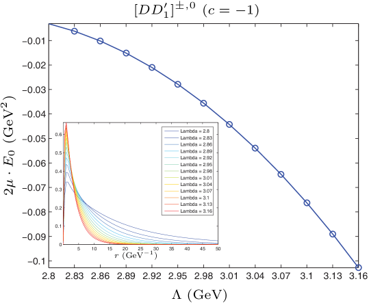
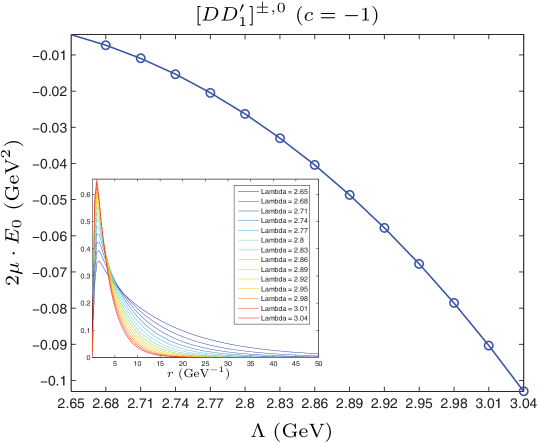
(a)	(b)

Figure 12: The binding energy of the $[DD_{1}^{\prime}]^{\pm,0}$ system $(c=-1)$ and the wave function of this system with $2h_{\sigma}$. Here, we only consider the $\sigma$ exchange potential. (a) and (b) correspond to the case of $g_{\sigma}g_{\sigma}^{\prime}>0$ and $g_{\sigma}g_{\sigma}^{\prime}<0$ with $|h_{\sigma}|=0.323$, $|g_{\sigma}|=0.76$ and $|g_{\sigma}^{\prime}|=0.76$ respectively.

When taking $2h_{\sigma}$, we present the variation of the binding energy of the $[PP_{1}^{\prime}]^{\pm,0}$ system with $c=-1$ and the cutoff $\Lambda$ in Fig. 12 in the cases $g_{\sigma}g_{\sigma}^{\prime}>0$ and $g_{\sigma}g_{\sigma}^{\prime}<0$. However, the corresponding cutoff $\Lambda$ is far larger than $1$ GeV. Thus, we tend to conclude that there does not exist a $[PP_{1}^{\prime}]^{\pm,0}$ bound state with $c=-1$.

III.2.2 $[PP_{1}^{\prime}]_{s}^{\pm,0},\,[PP_{1}^{\prime}]_{\hat{s}}^{0}$

There does not exist the $[PP_{1}^{\prime}]_{s}^{\pm,0},\,[PP_{1}^{\prime}]_{\hat{s}}^{0}$ bound state system since none of the meson exchange forces is allowed as indicated in Table 4.

III.2.3 $[PP_{1}^{\prime}]_{s1}^{0}$

(a)	(b)
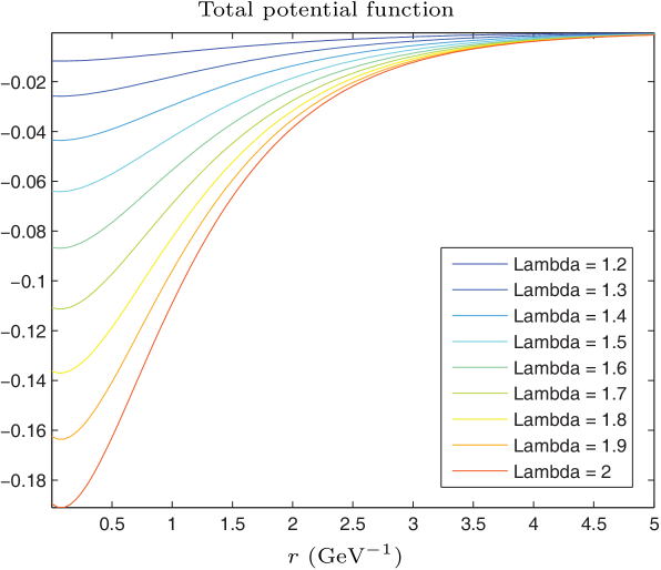
(c)	(d)

Figure 13: (a), (b), (c) and (d) are the potentials of the $[PP_{1}^{\prime}]_{s1}^{0}$ with $(c=+1,\,\beta\beta^{\prime}>0)$, $(c=+1,\,\beta\beta^{\prime}<0)$, $(c=-1,\,\beta\beta^{\prime}>0)$ and $(c=-1,\,\beta\beta^{\prime}<0)$, respectively. Here, we take $\zeta\varpi>0$ with $|\beta|=0.909$, $|\beta^{\prime}|=0.533$, $|\zeta|=0.727$ and $|\varpi|=0.364$.

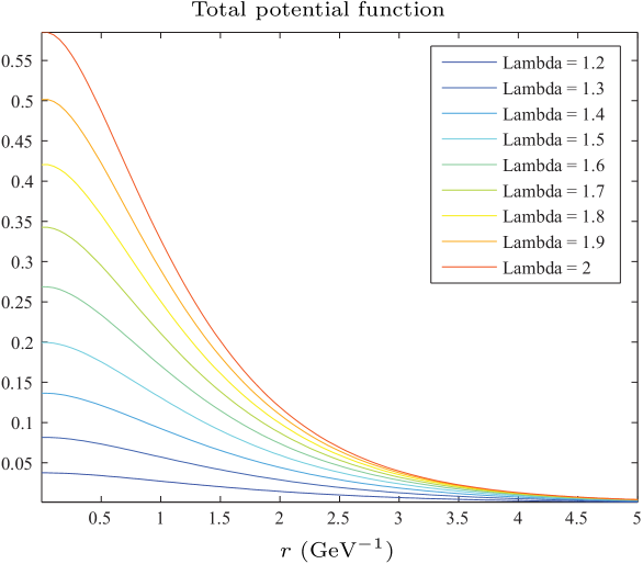
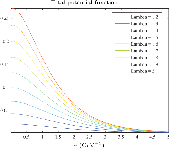
(a)	(b)
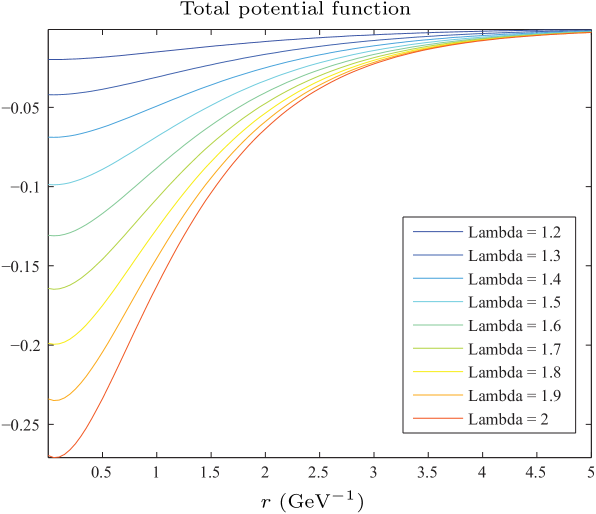
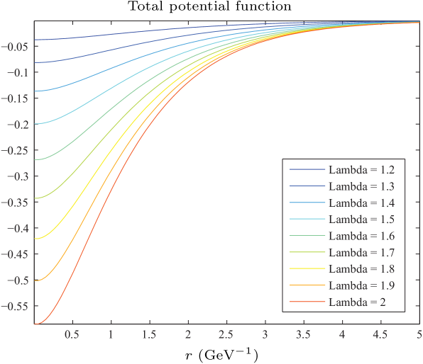
(c)	(d)

Figure 14: (a), (b), (c) and (d) are the potentials of the $[PP_{1}^{\prime}]_{s1}^{0}$ with $(c=+1,\,\beta\beta^{\prime}>0)$, $(c=+1,\,\beta\beta^{\prime}<0)$, $(c=-1,\,\beta\beta^{\prime}>0)$ and $(c=-1,\,\beta\beta^{\prime}<0)$, respectively. Here, we take $\zeta\varpi<0$ with $|\beta|=0.909$, $|\beta^{\prime}|=0.533$, $|\zeta|=0.727$ and $|\varpi|=0.364$.

Here the effective potential of the $[PP_{1}^{\prime}]_{s1}^{0}$ arises from the $\phi$ meson exchange. There exist eight combinations of the parameters $c$, $\beta\beta^{\prime}$ and $\zeta\varpi$. With different parameters, the dependence of the effective potential of the $[PP_{1}^{\prime}]_{s1}^{0}$ system with $c=\pm 1$ on $r$ is shown in Figs. 13-14.

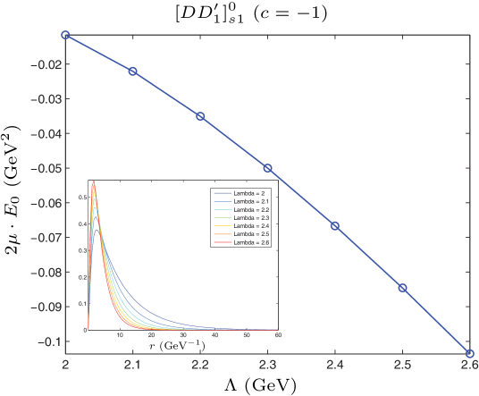
Figure 15: The dependence of the binding energy of the $[PP_{1}^{\prime}]_{s1}^{0}$ system on $\Lambda$ with $c=-1$, $\beta\beta^{\prime}<0$ and $\zeta\varpi<0$ with $|\beta|=0.909$, $|\beta^{\prime}|=0.533$, $|\zeta|=0.727$ and $|\varpi|=0.364$.

When solving the Schrödinger equation, the cutoff $\Lambda$ is expected to be larger than the mass of the $\phi$ meson. We only find bound state solutions of $[PP_{1}^{\prime}]_{s1}^{0}$ with $c=-1$, $\beta\beta^{\prime}<0$ and $\zeta\varpi<0$, which is shown in Fig. 15.

III.2.4 $[PP_{1}^{\prime}]_{8}^{0}$

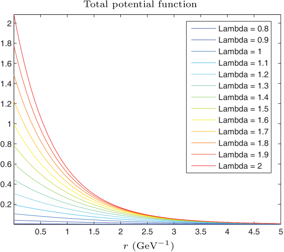
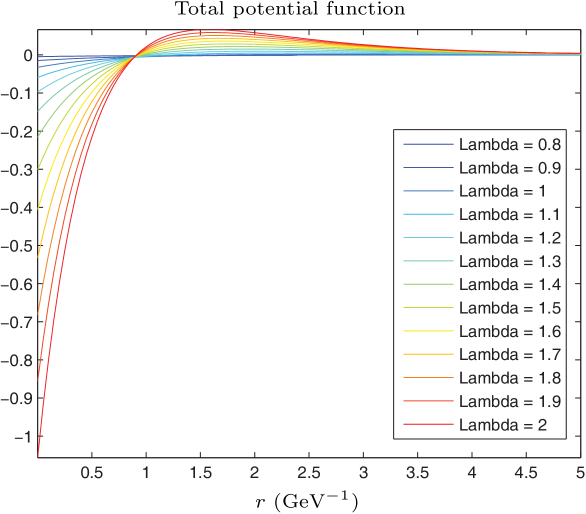
(a)	(b)
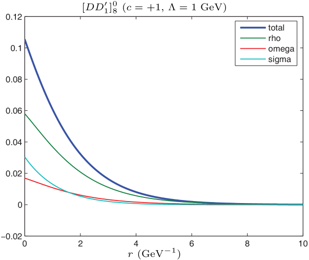
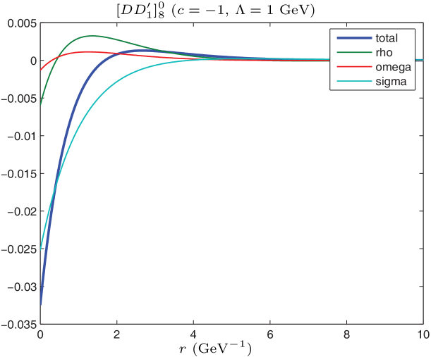
(c)	(d)

Figure 16: (a) and (b) are the total potentials of the $[PP_{1}^{\prime}]_{8}^{0}$ system with $c=+1$ and $c=-1$ respectively when $g_{\sigma}g_{\sigma}^{\prime}>0$, $\beta\beta^{\prime}>0$ and $\zeta\mu>0$ with $|\beta|=0.909$, $|\beta^{\prime}|=0.533$, $|\zeta|=0.727$ and $|\varpi|=0.364$. With $\Lambda=1$ GeV, we show the comparison of the total potential and the $\sigma,\,\rho,\,\omega$ exchange potentials, where (c) and (d) illustrate the result of the $[PP_{1}^{\prime}]_{8}^{0}$ system with $c=+1$ and $c=-1$ respectively.

The $\sigma$, $\rho$, $\omega$ exchange contributes to the total effective potential of $[PP_{1}^{\prime}]_{8}^{0}$ system. In Fig. 16, the variation of the total effective potential of $[PP_{1}^{\prime}]_{8}^{0}$ to $r$ and different typical $\Lambda$ values is given. The comparison of the total potential with the $\sigma$, $\rho$ and $\omega$ exchange potential is presented in Fig. 16 (c) and (d) with $\Lambda=1$ GeV.

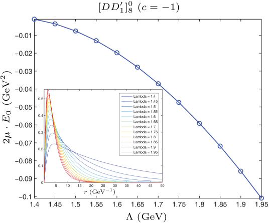
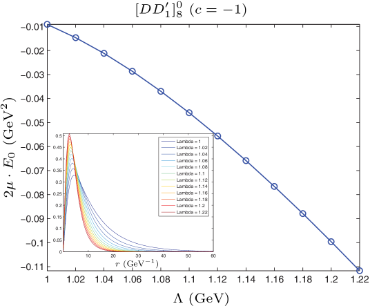
(a)	(b)
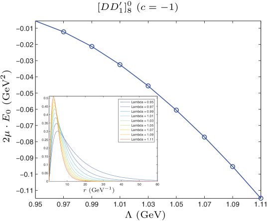
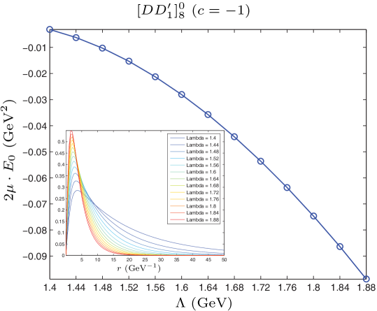
(c)	(d)
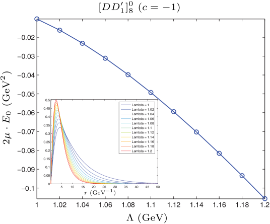
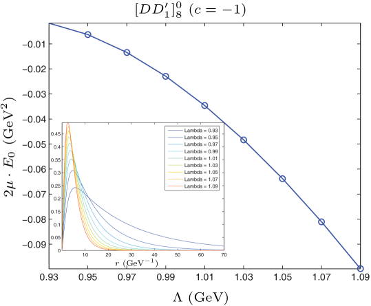
(e)	(f)

Figure 17: The bound state solution of the $[PP_{1}^{\prime}]_{8}^{0}$ with $c=-1$. (a), (b), (c), (d), (e), and (f) correspond to the results with $(g_{\sigma}g_{\sigma}^{\prime}>0,\,\beta\beta^{\prime}<0,\,\zeta\varpi>0)$, $(g_{\sigma}g_{\sigma}^{\prime}>0,\,\beta\beta^{\prime}>0,\,\zeta\varpi<0)$, $(g_{\sigma}g_{\sigma}^{\prime}>0,\,\beta\beta^{\prime}<0,\,\zeta\varpi<0)$, $(g_{\sigma}g_{\sigma}^{\prime}<0,\,\beta\beta^{\prime}<0,\,\zeta\varpi>0)$, $(g_{\sigma}g_{\sigma}^{\prime}<0,\,\beta\beta^{\prime}>0,\,\zeta\varpi<0)$ and $(g_{\sigma}g_{\sigma}^{\prime}<0,\,\beta\beta^{\prime}<0,\,\zeta\varpi<0)$ respectively. When taking $(g_{\sigma}g_{\sigma}^{\prime}>0,\,\beta\beta^{\prime}>0,\,\zeta\varpi>0)$ or $(g_{\sigma}g_{\sigma}^{\prime}<0,\,\beta\beta^{\prime}>0,\,\zeta\varpi>0)$, we can not find the bound state solution. Here, $|g_{\sigma}|=0.76$, $|g_{\sigma}^{\prime}|=0.76$, $|h_{\sigma}|=0.323$, $|\beta|=0.909$ and $|\beta^{\prime}|=0.533$, $\zeta=0.727$ and $\varpi=0.364$.

Since the total potential is repulsive for the case of $c=+1$, we only explore wether there exists the bound state $[PP_{1}^{\prime}]_{8}^{0}$ system with $c=-1$. The combinations of coupling constants $g_{\sigma}g_{\sigma}^{\prime}$, $\beta\beta^{\prime}$ and $\zeta\varpi$ are eight. However, we find the bound state solution of $[PP_{1}^{\prime}]_{8}^{0}$ system with $c=-1$ with six parameter combinations just listed in the caption of Fig. 17.

III.3 The $[P^{*}P_{0}^{*}]$ system

III.3.1 $[P^{*}P_{0}^{*}]^{\pm,0}$

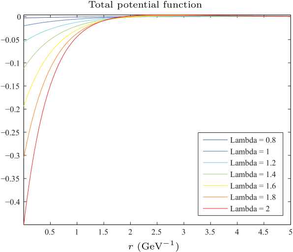
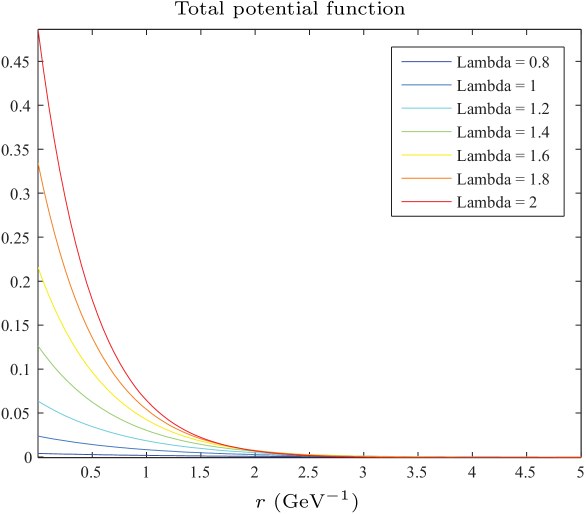
(a)	(b)
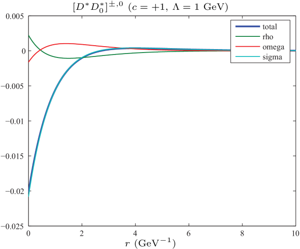
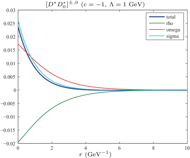
(c)	(d)

Figure 18: (a) The variation of the total potential of the $[D^{*}D_{0}^{*}]^{\pm,0}$ system $(c=+1)$ with $r$ and $\Lambda$; (b) the variation of the total potential of the $[D^{*}D_{0}^{*}]^{\pm,0}$ system $(c=-1)$ with $r$ and $\Lambda$; (c) the exchange potentials of the $\sigma,\,\rho,\,\omega$ mesons of the $[DD_{1}^{\prime}]^{\pm,0}$ system $(c=+1)$ with $\Lambda=1$ GeV; (d) the exchange potentials of the $\sigma,\,\rho,\,\omega$ mesons of the $[D^{*}D_{0}^{*}]^{\pm,0}$ system $(c=-1)$ with $\Lambda=1$ GeV. The above potentials are obtained with $g_{\sigma}g_{\sigma}^{\prime}>0$, $\beta\beta^{\prime}>0$ and $\zeta\varpi>0$. Here, $|g_{\sigma}|=0.76$, $|g_{\sigma}^{\prime}|=0.76$, $|h_{\sigma}|=0.32$, $|\beta|=0.909$ and $|\beta^{\prime}|=0.533$, $\zeta=0.727$ and $\varpi=0.364$.

The total effective potential of the $[P^{*}P_{0}^{*}]^{\pm,0}$ system arises from the $\sigma$, $\rho$ and $\omega$ meson exchange. Since the $\rho$ and $\omega$ exchange potentials cancel each other, the $\sigma$ exchange potential is dominant in the total effective potential of $[P^{*}P_{0}^{*}]^{\pm,0}$. We only consider the $\omega$ exchange potential contribution to explore whether there exists a $[P^{*}P_{0}^{*}]^{\pm,0}$ bound state . In Fig. 18, the effective potential of the $[P^{*}P_{0}^{*}]^{\pm,0}$ system is presented.

The $\sigma$ exchange potential of $[PP_{1}^{\prime}]^{\pm,0}$ system with $c=-1$ is repulsive. Thus there does not exist a $[PP_{1}^{\prime}]^{\pm,0}$ bound state with $c=-1$.

For the $[P^{*}P_{0}^{*}]^{\pm,0}$ system with $c=+1$, the $\sigma$ exchange potential is attractive. Meanwhile, the cross diagram plays the dominant role to the $\sigma$ exchange potential. However, in the $g_{\sigma}g_{\sigma}^{\prime}>0$ and $g_{\sigma}g_{\sigma}^{\prime}<0$ two cases, we can not find bound state solutions of the $[P^{*}P_{0}^{*}]^{\pm,0}$ system with $c=-1$ and the coupling constants listed in the caption of Fig. 18 when scanning the range of the cutoff $\Lambda$.

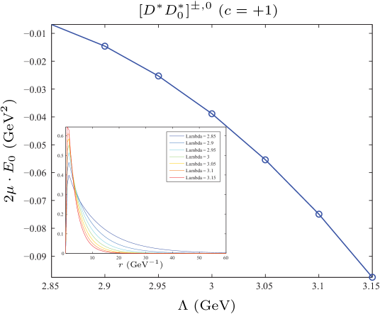
Figure 19: The binding energy of the $[D^{*}D_{0}^{*}]^{\pm,0}$ system $(c=+1)$ and its wave function with $2h_{\sigma}$. Here, we only consider the $\sigma$ exchange potential and take $g_{\sigma}g_{\sigma}^{\prime}<0$ with $|h_{\sigma}|=0.323$, $|g_{\sigma}|=0.76$ and $|g_{\sigma}^{\prime}|=0.76$.

When taking $2h_{\sigma}$, we obtain the binding energy of the $[P^{*}P_{0}^{*}]^{\pm,0}$ system with $c=+1$ dependent on the cutoff $\Lambda$ in Fig. 19 only in the $g_{\sigma}g_{\sigma}^{\prime}<0$ case. However, the corresponding cutoff $\Lambda$ is far larger than usual $1$ GeV. Thus, the $[P^{*}P_{0}^{*}]^{\pm,0}$ system with $c=+1$ seems impossible to form the bound state.

III.3.2 $[P^{*}P_{0}^{*}]_{s}^{\pm,0},\,[P^{*}P_{0}^{*}]_{\hat{s}}^{0}$

There does not exist the $[P^{*}P_{0}^{*}]_{s}^{\pm,0},\,[P^{*}P_{0}^{*}]_{\hat{s}}^{0}$ bound state since no suitable meson exchange force is allowed as indicated in Table 4.

III.3.3 $[P^{*}P_{0}^{*}]_{s1}^{0}$

(a)	(b)
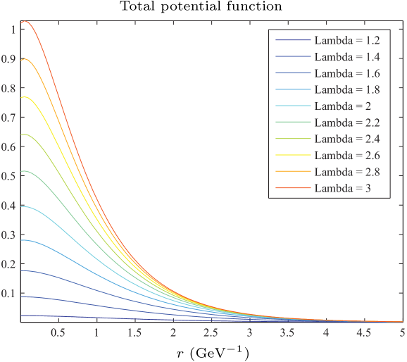
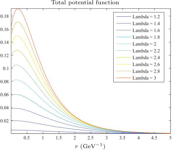
(c)	(d)

Figure 21: (a), (b), (c) and (d) are the potentials of the $[D^{*}D_{0}^{*}]_{s1}^{0}$ system with $(c=+1,\,\beta\beta^{\prime}>0)$, $(c=+1,\,\beta\beta^{\prime}<0)$, $(c=-1,\,\beta\beta^{\prime}>0)$ and $(c=-1,\,\beta\beta^{\prime}<0)$, respectively. Here, we take $\zeta\varpi<0$ with $|\beta|=0.909$, $|\beta^{\prime}|=0.533$, $|\zeta|=0.727$ and $|\varpi|=0.364$.

Here, the effective potential of the $[P^{*}P_{0}^{*}]_{s1}^{0}$ system results from the $\phi$ meson exchange. There exist eight combinations of the parameters $c$, $\beta\beta^{\prime}$ and $\zeta\varpi$. Under different parameter space, the dependence of the effective potential of $[P^{*}P_{0}^{*}]_{s1}^{0}$ with $c=\pm 1$ on $r$ is listed in Figs. 20-21.

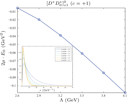
Figure 22: The dependence of the binding energy of $[D^{*}D_{0}^{*}]_{s1}^{0}$ on $\Lambda$ with $c=+1$, $\beta\beta^{\prime}<0$ and $\zeta\varpi<0$ with $|\beta|=0.909$, $|\beta^{\prime}|=0.533$, $|\zeta|=0.727$ and $|\varpi|=0.364$.

When solving the Schrödinger equation, the cutoff $\Lambda$ should be larger than the mass of the $\phi$ meson. There exists a bound state solution of the $[P^{*}P_{0}^{*}]_{s1}^{0}$ system only with $c=+1$, $\beta\beta^{\prime}<0$ and $\zeta\varpi<0$, which is shown in Fig. 22.

III.3.4 $[P^{*}P_{0}^{*}]_{8}^{0}$

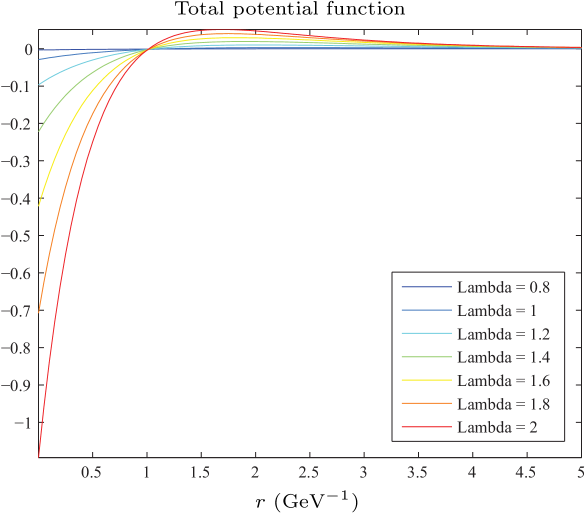
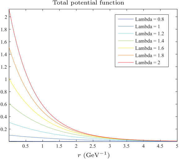
(a)	(b)
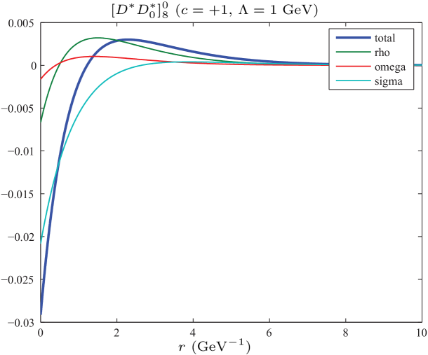
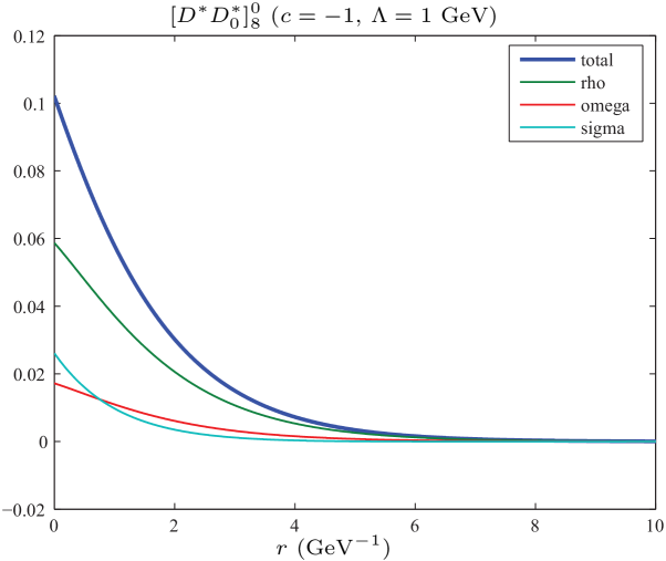
(c)	(d)

Figure 23: (a) and (b) are the total potentials of the $[D^{*}D_{0}^{*}]_{8}^{0}$ system with $c=+1$ and $c=-1$ respectively with $g_{\sigma}g_{\sigma}^{\prime}>0$, $\beta\beta^{\prime}>0$ and $\zeta\mu>0$ with $|\beta|=0.909$, $|\beta^{\prime}|=0.533$, $|\zeta|=0.727$ and $|\varpi|=0.364$. With $\Lambda=1$ GeV, we show the comparison of the total potential and the $\sigma,\,\rho,\,\omega$ exchange potentials, where (c) and (d) illustrate the result of the $[D^{*}D_{0}^{*}]_{8}^{0}$ system with $c=+1$ and $c=-1$ respectively.

As indicated in Table 4, the behavior of the $\rho$ meson exchange potential is similar to that of the $\omega$ meson exchange potential. When exploring the $[P^{*}P_{0}^{*}]_{8}^{0}$ system, we need to consider the $\sigma$ exchange potential together with both the $\rho$ and $\omega$ meson exchanges. The relevant total and partial potentials are shown in Fig. 23.

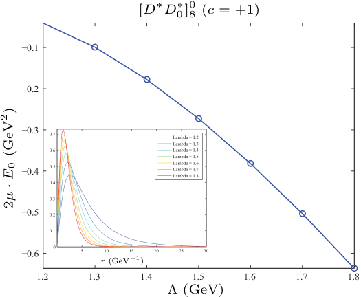
(a)	(b)
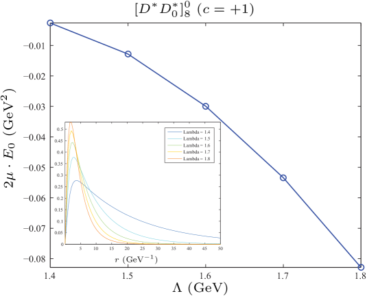
(c)	(d)
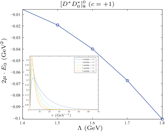
(e)	(f)

Figure 24: The bound state solution of the $[D^{*}D_{0}^{*}]_{8}^{0}$ with $c=+1$. (a), (b), (c), (d), (e), and (f) correspond to the results with $(g_{\sigma}g_{\sigma}^{\prime}>0,\,\beta\beta^{\prime}<0,\,\zeta\varpi>0)$, $(g_{\sigma}g_{\sigma}^{\prime}>0,\,\beta\beta^{\prime}<0,\,\zeta\varpi<0)$, $(g_{\sigma}g_{\sigma}^{\prime}>0,\,\beta\beta^{\prime}>0,\,\zeta\varpi<0)$, $(g_{\sigma}g_{\sigma}^{\prime}<0,\,\beta\beta^{\prime}<0,\,\zeta\varpi>0)$, $(g_{\sigma}g_{\sigma}^{\prime}<0,\,\beta\beta^{\prime}>0,\,\zeta\varpi<0)$ and $(g_{\sigma}g_{\sigma}^{\prime}<0,\,\beta\beta^{\prime}<0,\,\zeta\varpi<0)$ respectively. When taking $(g_{\sigma}g_{\sigma}^{\prime}>0,\,\beta\beta^{\prime}>0,\,\zeta\varpi>0)$ or $(g_{\sigma}g_{\sigma}^{\prime}<0,\,\beta\beta^{\prime}>0,\,\zeta\varpi>0)$, we can not find the bound state solution. Here, $|g_{\sigma}|=0.76$, $|g_{\sigma}^{\prime}|=0.76$, $|h_{\sigma}|=0.323$, $|\beta|=0.909$ and $|\beta^{\prime}|=0.533$, $\zeta=0.727$ and $\varpi=0.364$.

Since the total potential of the $[P^{*}P_{0}^{*}]_{8}^{0}$ system with $c=-1$ is repulsive, there does not exist a $[P^{*}P_{0}^{*}]_{8}^{0}$ bound state system with $c=-1$. In the following, we mainly focus on the $[P^{*}P_{0}^{*}]_{8}^{0}$ system with $c=+1$, where the total effective potential is attractive. As shown in Fig. 24, there exists the bound state solution of the $[P^{*}P_{0}^{*}]_{8}^{0}$ system with $c=+1$.

III.4 The $[P^{*}P_{1}^{\prime}]$ system

In Refs. liu3 ; liu4 ; close1 , the $[P^{*}P_{1}^{\prime}]^{\pm,0}$ and $[P^{*}P_{1}^{\prime}]_{8}^{0}$ systems were studied. In this work we will discuss the rest two cases of the $[P^{*}P_{1}^{\prime}]$ system, i.e., $[P^{*}P_{1}^{\prime}]_{s}^{\pm,0}/[P^{*}P_{1}^{\prime}]_{\hat{s}}^{0}$ and $[P^{*}P_{0}^{\prime}]_{s1}^{0}$.

III.4.1 $[P^{*}P_{1}^{\prime}]_{s}^{\pm,0},\,[P^{*}P_{1}^{\prime}]_{\hat{s}}^{0}$

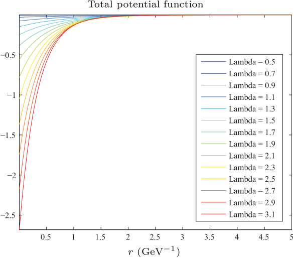
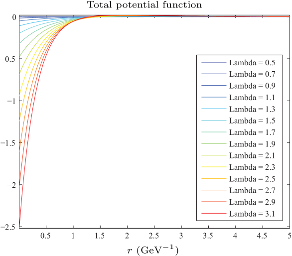
(a)	(b)
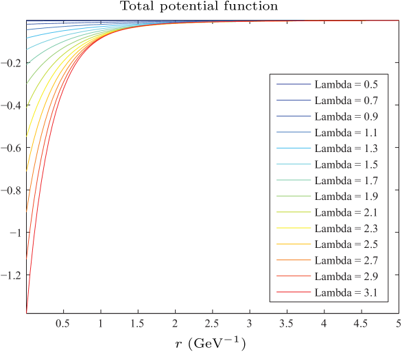
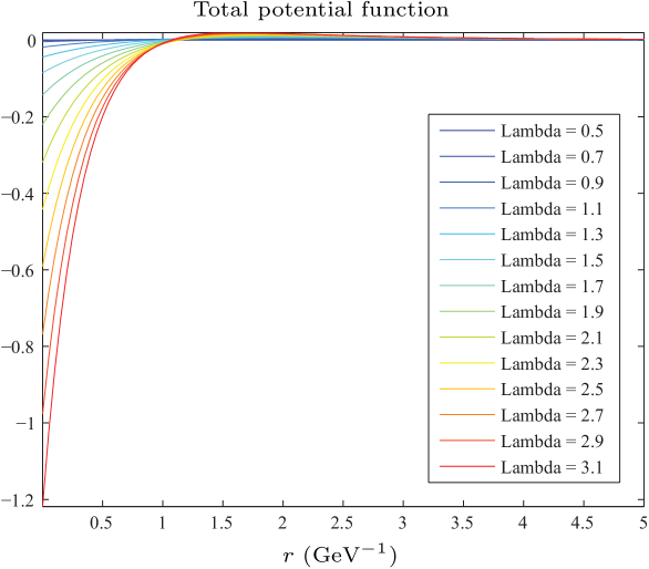
(c)	(d)
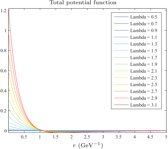
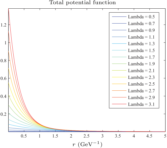
(e)	(f)

Figure 25: The variation of the potential of the $[D^{*}D_{1}^{\prime}]_{s}^{\pm,0}$, $[D^{*}D_{1}^{\prime}]_{\hat{s}}^{0}$ system, where we only list several typical cases with parameters $(c=+1,\,J=0,\,gg^{\prime}>0)$, $(c=-1,\,J=0,\,gg^{\prime}>0)$, $(c=+1,\,J=1,\,gg^{\prime}>0)$, $(c=-1,\,J=1,\,gg^{\prime}>0)$, $(c=+1,\,J=2,\,gg^{\prime}>0)$ and $(c=-1,\,J=0,\,gg^{\prime}>0)$, which correspond to diagrams (a), (b), (c), (d), (e) and (f) respectively. The above results are obtained with $1h$. Here, $|h|=0.56$, $|g|=0.75$ and $|g^{\prime}|=0.25$.

The effective potential of the $[P^{*}P_{1}^{\prime}]_{s}^{\pm,0},\,[P^{*}P_{1}^{\prime}]_{\hat{s}}^{0}$ system arises from the $\eta$ meson exchange only, which is plotted in Fig. 25 under several typical combinations of parameters.

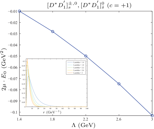
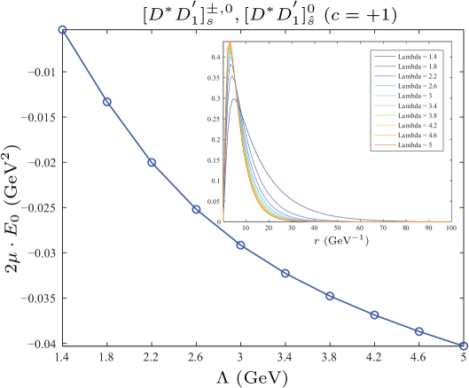
(a)	(b)
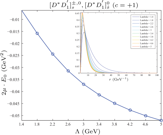
(c)	(d)
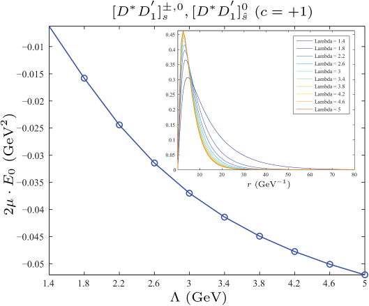
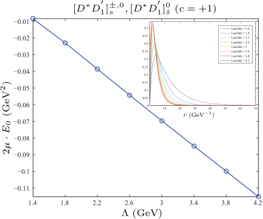
(e)	(f)

Figure 26: The bound state solutions of the $[D^{*}D_{1}^{\prime}]_{s}^{\pm,0}$, $[D^{*}D_{1}^{\prime}]_{\hat{s}}^{0}$ system with $(c=+1,\,J=0,\,gg^{\prime}>0)$, $(c=+1,\,J=0,\,gg^{\prime}<0)$, $(c=+1,\,J=1,\,gg^{\prime}>0)$, $(c=+1,\,J=1,\,gg^{\prime}<0)$, $(c=+1,\,J=2,\,gg^{\prime}>0)$ and $(c=+1,\,J=0,\,gg^{\prime}<0)$, which correspond to diagrams (a), (b), (c), (d), (e) and (f) respectively. The above numerical results are obtained with $3h$ while we can not find the bound state solution for $1h$ and $2h$. Here, $|h|=0.56$, $|g|=0.75$ and $|g^{\prime}|=0.25$.

When solving the the Schrödinger equation, we obtain the bound state solutions of the $[D^{*}D_{1}^{\prime}]_{s}^{\pm,0}$, $[D^{*}D_{1}^{\prime}]_{\hat{s}}^{0}$ system, which are listed in Fig. 26. The bound state solution of the $[D^{*}D_{1}^{\prime}]_{s}^{\pm,0}$, $[D^{*}D_{1}^{\prime}]_{\hat{s}}^{0}$ system appears when $(c=+1,\,J=0,\,gg^{\prime}>0)$, $(c=+1,\,J=0,\,gg^{\prime}<0)$, $(c=+1,\,J=1,\,gg^{\prime}>0)$, $(c=+1,\,J=1,\,gg^{\prime}<0)$, $(c=+1,\,J=2,\,gg^{\prime}>0)$ and $(c=+1,\,J=0,\,gg^{\prime}<0)$. The above numerical results are obtained with $3h$ while we can not find the bound state solution for $1h$ and $2h$.

III.4.2 $[P^{*}P_{0}^{\prime}]_{s1}^{0}$

(a)	(b)
(c)	(d)
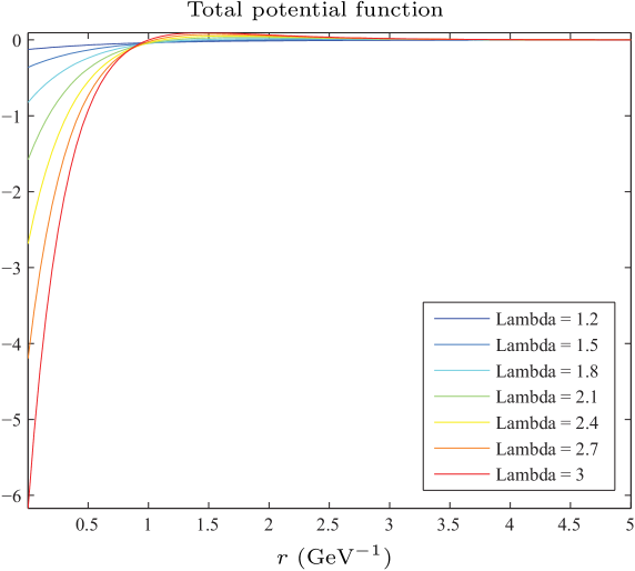
(e)	(f)

Figure 27: The variation of the potential of the $[D^{*}D_{1}^{\prime}]_{s1}^{0}$ system with $r$. (a), (b), (c), (d), (e) and (f) are for parameters $(c=+1,\,J=0,\,\beta\beta^{\prime}>0,\,\lambda\lambda^{\prime}>0,\,\zeta\varpi>0)$, $(c=-1,\,J=0,\,\beta\beta^{\prime}>0,\,\lambda\lambda^{\prime}>0,\,\zeta\varpi>0)$, $(c=+1,\,J=1,\,\beta\beta^{\prime}>0,\,\lambda\lambda^{\prime}>0,\,\zeta\varpi>0)$, $(c=-1,\,J=1,\,\beta\beta^{\prime}>0,\,\lambda\lambda^{\prime}>0,\,\zeta\varpi>0)$, $(c=+1,\,J=2,\,\beta\beta^{\prime}>0,\,\lambda\lambda^{\prime}>0,\,\zeta\varpi>0)$ and $(c=-1,\,J=2,\,\beta\beta^{\prime}>0,\,\lambda\lambda^{\prime}>0,\,\zeta\varpi>0)$, respectively. Here, $|h|=0.56$, $|g|=0.75$, $|g^{\prime}|=0.25$, $|\lambda|=0.4546$, $|\lambda^{\prime}|=0.2667$, $|\beta|=0.909$, $|\beta^{\prime}|=0.533$, $|\zeta|=0.727$ and $|\varpi|=0.364$.

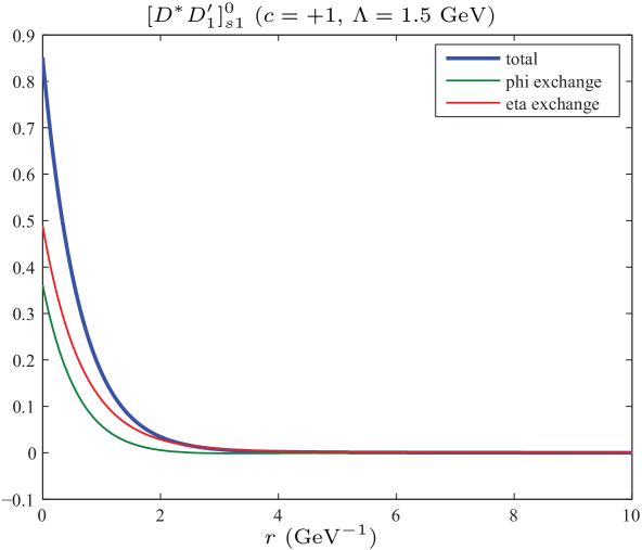
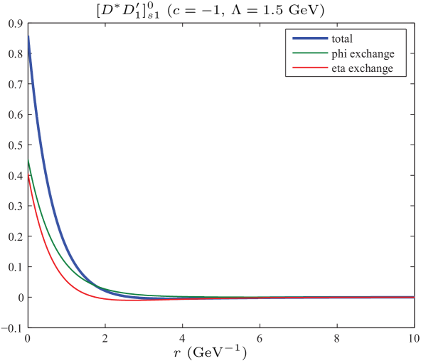
(a)	(b)
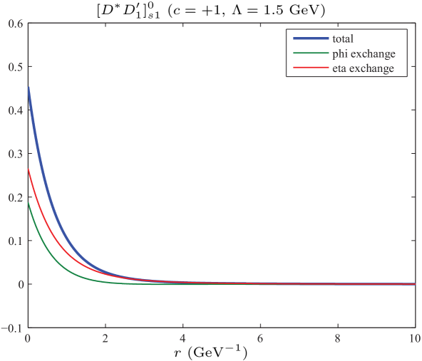
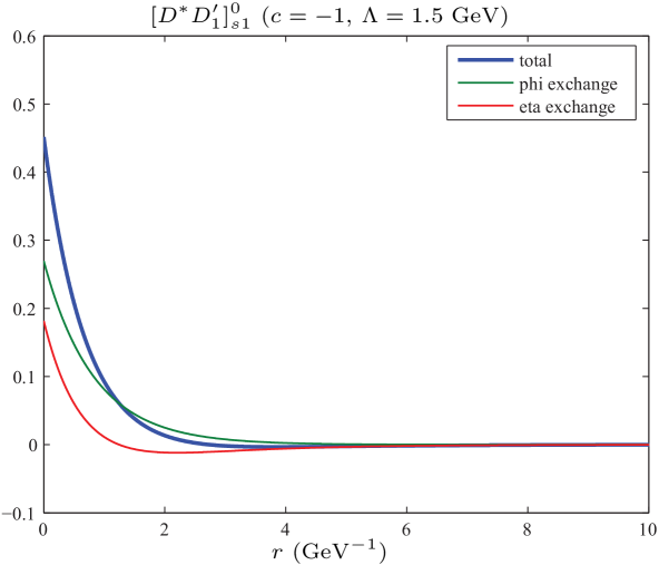
(c)	(d)
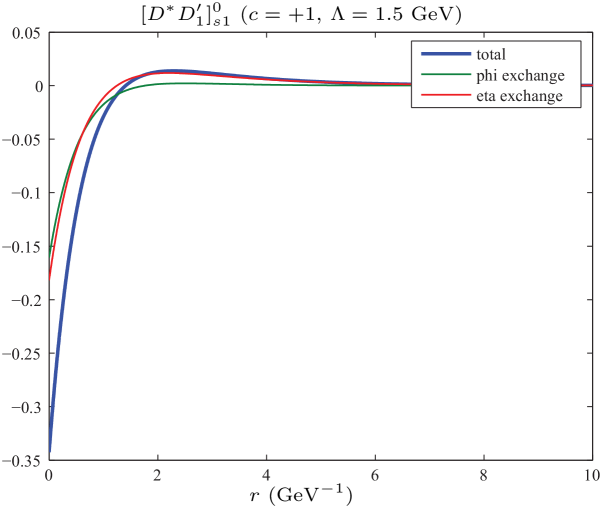
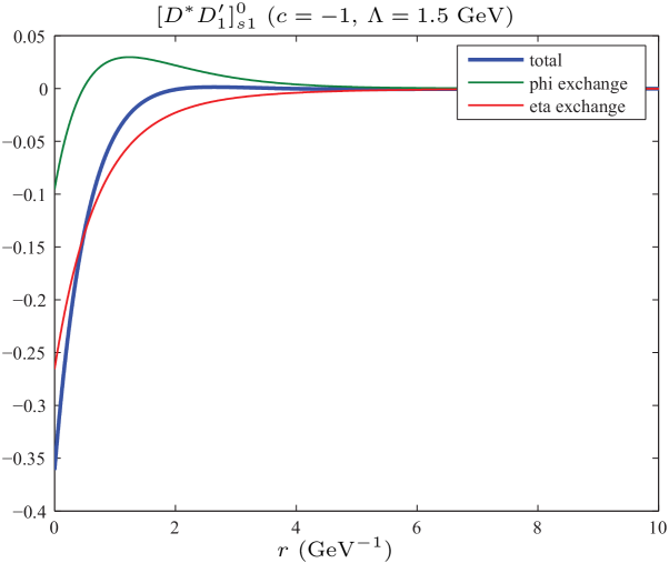
(e)	(f)

Figure 28: The comparison of the $\eta$ and $\phi$ exchange potentials with the total effective potential for the $[D^{*}D_{1}^{\prime}]_{s1}^{0}$ system with $\Lambda=1.5$ GeV. (a), (b), (c), (d), (e) and (f) are for parameters $(c=+1,\,J=0,\,\beta\beta^{\prime}>0,\,\lambda\lambda^{\prime}>0,\,gg^{\prime}>0,\,\zeta\varpi>0)$, $(c=-1,\,J=0,\,\beta\beta^{\prime}>0,\,\lambda\lambda^{\prime}>0,\,gg^{\prime}>0,\,\zeta\varpi>0)$, $(c=+1,\,J=1,\,\beta\beta^{\prime}>0,\,\lambda\lambda^{\prime}>0,\,gg^{\prime}>0,\,\zeta\varpi>0)$, $(c=-1,\,J=1,\,\beta\beta^{\prime}>0,\,\lambda\lambda^{\prime}>0,\,gg^{\prime}>0,\,\zeta\varpi>0)$, $(c=+1,\,J=2,\,\beta\beta^{\prime}>0,\,\lambda\lambda^{\prime}>0,\,gg^{\prime}>0,\,\zeta\varpi>0)$ and $(c=-1,\,J=2,\,\beta\beta^{\prime}>0,\,\lambda\lambda^{\prime}>0,\,gg^{\prime}>0,\,\zeta\varpi>0)$, respectively. Here, $|h|=0.56$, $|g|=0.75$, $|g^{\prime}|=0.25$, $|\lambda|=0.4546$, $|\lambda^{\prime}|=0.2667$, $|\beta|=0.909$, $|\beta^{\prime}|=0.533$, $|\zeta|=0.727$ and $|\varpi|=0.364$.

The effective potential of the $[P^{*}P_{1}^{\prime}]_{s1}^{0}$ system results from both the $\eta$ and $\phi$ meson exchanges as shown in Figs. 27 and 28.

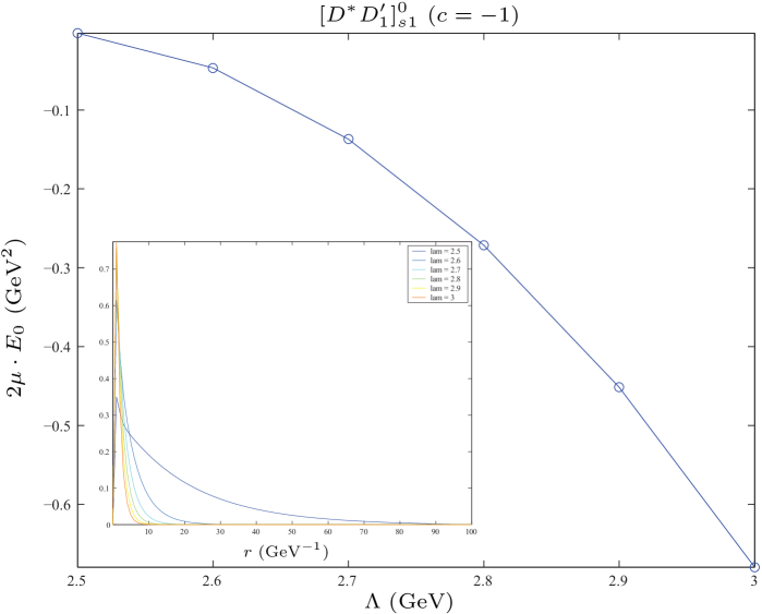
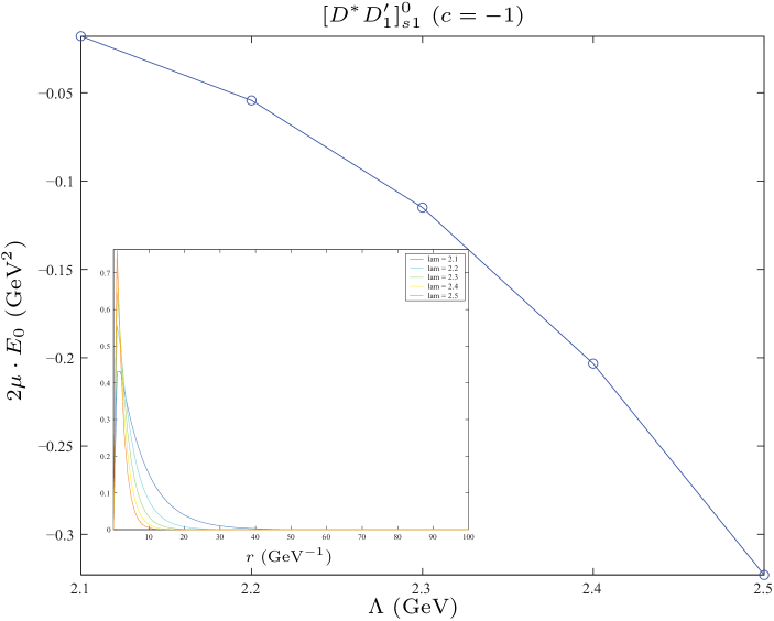
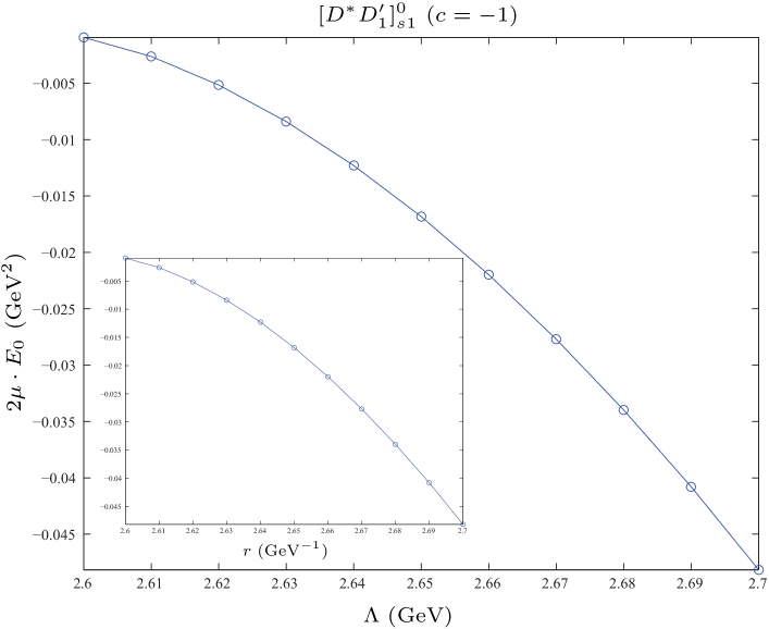
(a)	(b)	(c)
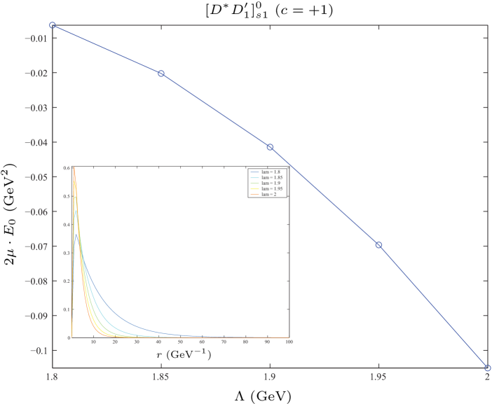
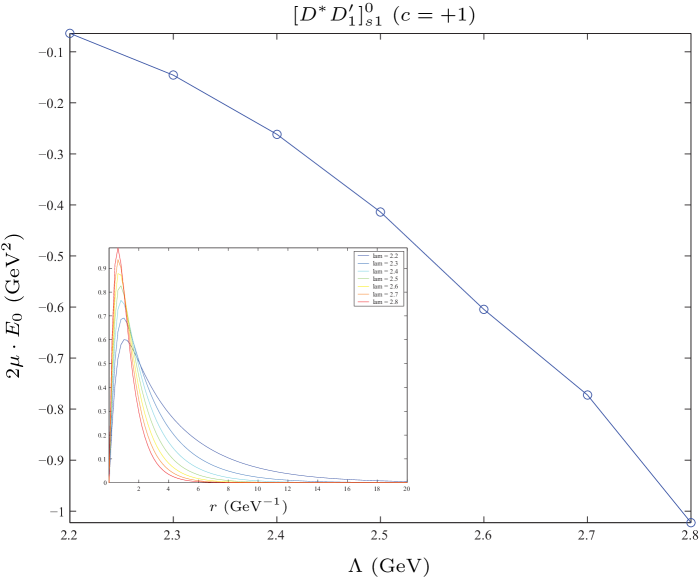
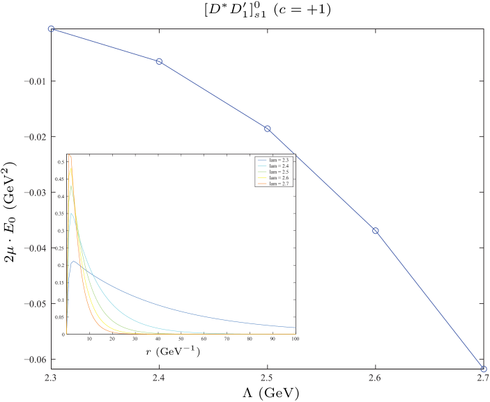
(d)	(e)	(f)
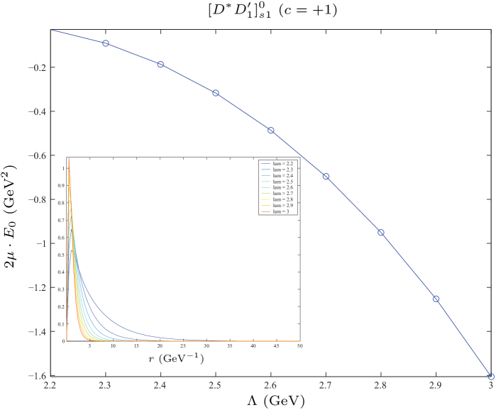
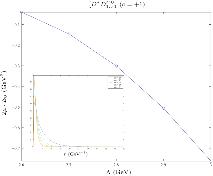
(g)	(h)

Figure 29: The bound state solution of the $[D^{*}D_{1}^{\prime}]_{s1}^{0}$ system with $(c=-1,\,J=0,\,\beta\beta^{\prime}<0,\,\lambda\lambda^{\prime}<0,\,gg^{\prime}<0,\,\zeta\varpi<0)$, $(c=-1,\,J=0,\,\beta\beta^{\prime}<0,\,\lambda\lambda^{\prime}<0,\,gg^{\prime}<0,\,\zeta\varpi>0)$, $(c=-1,\,J=0,\,\beta\beta^{\prime}>0,\,\lambda\lambda^{\prime}<0,\,gg^{\prime}<0,\,\zeta\varpi>0)$, $(c=+1,\,J=0,\,\beta\beta^{\prime}<0,\,\lambda\lambda^{\prime}<0,\,gg^{\prime}<0,\,\zeta\varpi<0)$, $(c=+1,\,J=0,\,\beta\beta^{\prime}<0,\,\lambda\lambda^{\prime}<0,\,gg^{\prime}<0,\,\zeta\varpi>0)$, $(c=+1,\,J=0,\,\beta\beta^{\prime}<0,\,\lambda\lambda^{\prime}<0,\,gg^{\prime}>0,\,\zeta\varpi<0)$, $(c=+1,\,J=0,\,\beta\beta^{\prime}>0,\,\lambda\lambda^{\prime}<0,\,gg^{\prime}<0,\,\zeta\varpi<0)$ and $(c=+1,\,J=0,\,\beta\beta^{\prime}>0,\,\lambda\lambda^{\prime}<0,\,gg^{\prime}<0,\,\zeta\varpi>0)$, which correspond to diagrams (a), (b), (c), (d), (e), (f), (g) and (h) respectively. Here, we take $1h$. $|h|=0.56$, $|g|=0.75$, $|g^{\prime}|=0.25$, $|\lambda|=0.4546$, $|\lambda^{\prime}|=0.2667$, $|\beta|=0.909$, $|\beta^{\prime}|=0.533$, $|\zeta|=0.727$ and $|\varpi|=0.364$.

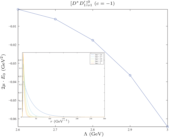
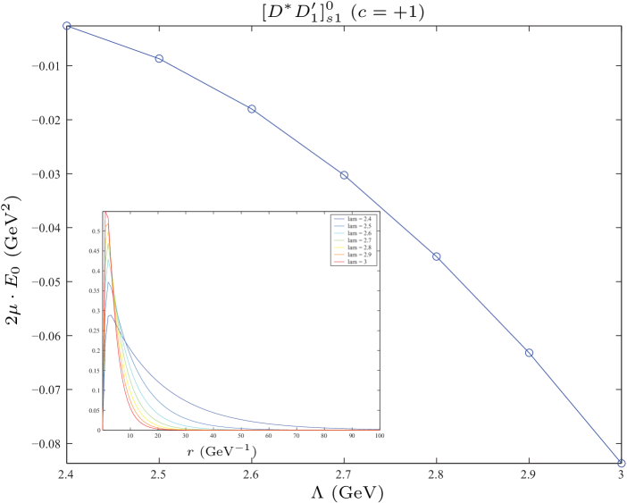
(a)	(b)
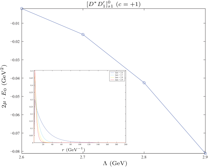
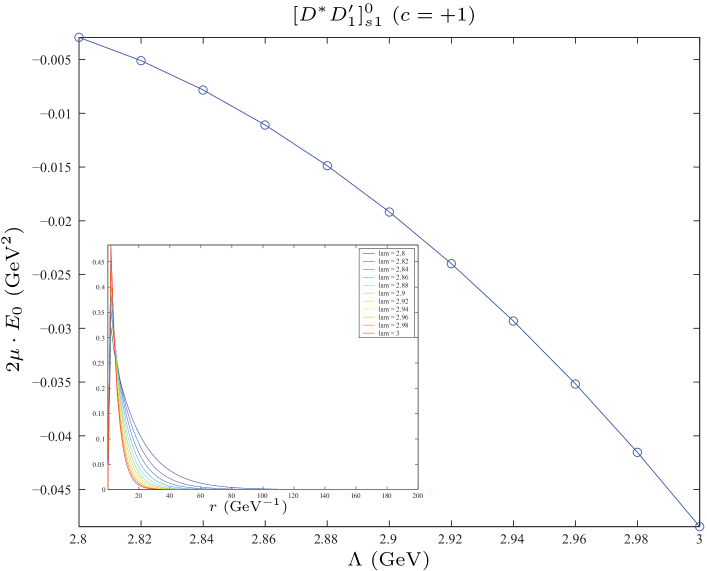
(c)	(d)
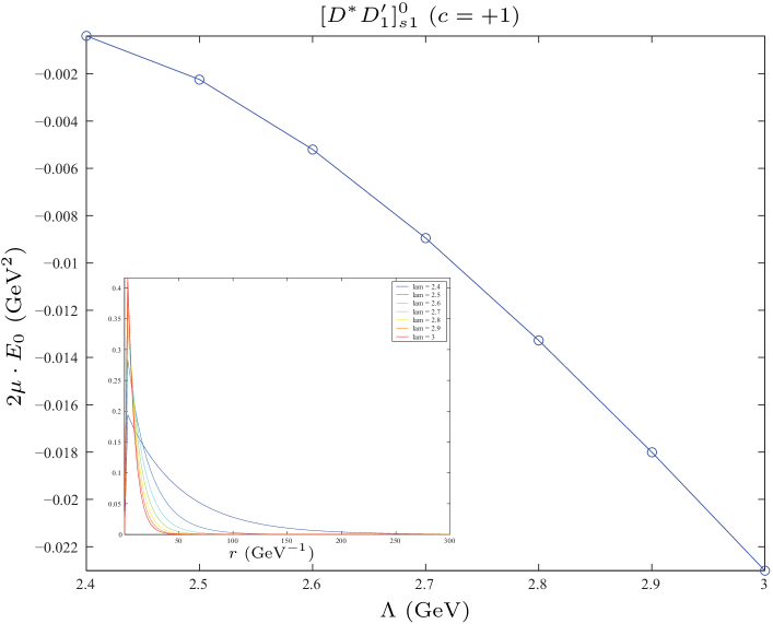
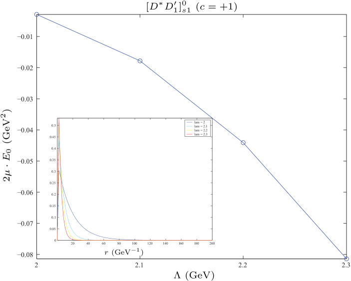
(e)	(f)

Figure 30: The bound state solution of the $[D^{*}D_{1}^{\prime}]_{s1}^{0}$ system with $(c=-1,\,J=1,\,\beta\beta^{\prime}<0,\,\lambda\lambda^{\prime}<0,\,gg^{\prime}<0,\,\zeta\varpi>0)$, $(c=+1,\,J=1,\,\beta\beta^{\prime}>0,\,\lambda\lambda^{\prime}<0,\,gg^{\prime}>0,\,\zeta\varpi<0)$, $(c=+1,\,J=1,\,\beta\beta^{\prime}>0,\,\lambda\lambda^{\prime}<0,\,gg^{\prime}<0,\,\zeta\varpi>0)$, $(c=+1,\,J=1,\,\beta\beta^{\prime}>0,\,\lambda\lambda^{\prime}<0,\,gg^{\prime}<0,\,\zeta\varpi<0)$, $(c=+1,\,J=1,\,\beta\beta^{\prime}<0,\,\lambda\lambda^{\prime}>0,\,gg^{\prime}<0,\,\zeta\varpi<0)$ and $(c=+1,\,J=1,\,\beta\beta^{\prime}<0,\,\lambda\lambda^{\prime}<0,\,gg^{\prime}<0,\,\zeta\varpi<0)$, which correspond to diagrams (a), (b), (c), (d), (e) and (f) respectively. Here, we use $1h$. $|h|=0.56$, $|g|=0.75$, $|g^{\prime}|=0.25$, $|\lambda|=0.4546$, $|\lambda^{\prime}|=0.2667$, $|\beta|=0.909$, $|\beta^{\prime}|=0.533$, $|\zeta|=0.727$ and $|\varpi|=0.364$.

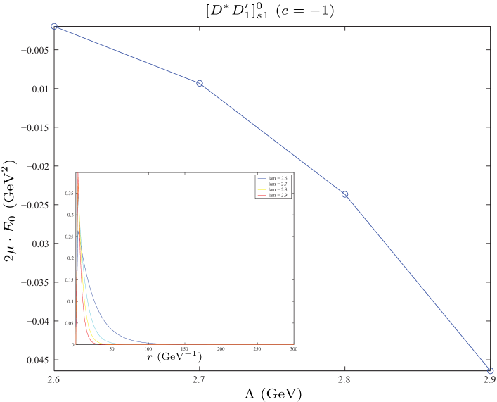
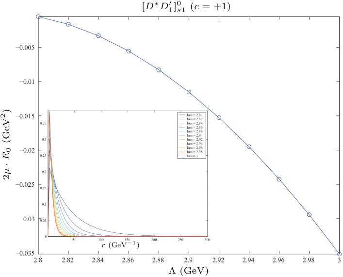
(a)	(b)
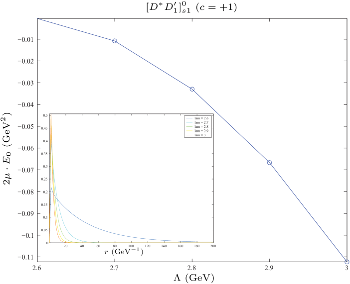
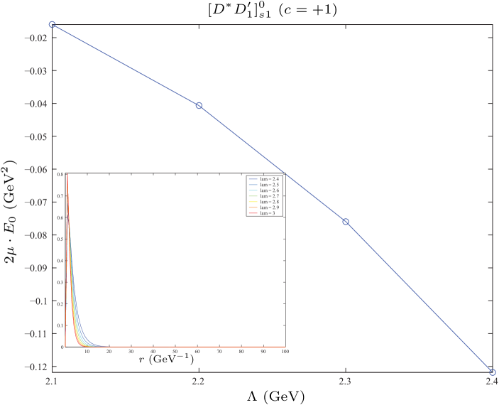
(c)	(d)
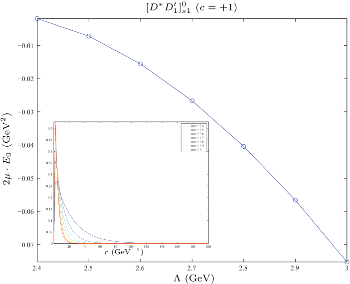
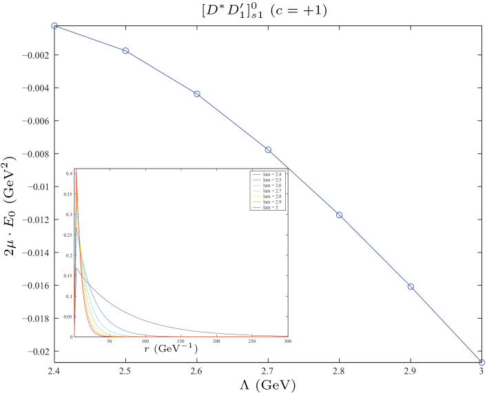
(e)	(f)

Figure 31: The bound state solution of the $[D^{*}D_{1}^{\prime}]_{s1}^{0}$ system with $(c=-1,\,J=2,\,\beta\beta^{\prime}<0,\,\lambda\lambda^{\prime}>0,\,gg^{\prime}>0,\,\zeta\varpi>0)$, $(c=+1,\,J=2,\,\beta\beta^{\prime}>0,\,\lambda\lambda^{\prime}>0,\,gg^{\prime}>0,\,\zeta\varpi<0)$, $(c=+1,\,J=2,\,\beta\beta^{\prime}<0,\,\lambda\lambda^{\prime}>0,\,gg^{\prime}>0,\,\zeta\varpi>0)$, $(c=+1,\,J=2,\,\beta\beta^{\prime}<0,\,\lambda\lambda^{\prime}>0,\,gg^{\prime}>0,\,\zeta\varpi<0)$, $(c=+1,\,J=2,\,\beta\beta^{\prime}<0,\,\lambda\lambda^{\prime}>0,\,gg^{\prime}<0,\,\zeta\varpi<0)$ and $(c=+1,\,J=2,\,\beta\beta^{\prime}<0,\,\lambda\lambda^{\prime}<0,\,gg^{\prime}>0,\,\zeta\varpi<0)$, which correspond to diagrams (a), (b), (c), (d), (e) and (f) respectively. Here, we use $1h$. $|h|=0.56$, $|g|=0.75$, $|g^{\prime}|=0.25$, $|\lambda|=0.4546$, $|\lambda^{\prime}|=0.2667$, $|\beta|=0.909$, $|\beta^{\prime}|=0.533$, $|\zeta|=0.727$ and $|\varpi|=0.364$.

There exist 96 combinations of the parameters $c$, $\beta\beta^{\prime}$, $gg^{\prime}$, $\lambda\lambda^{\prime}$ and $\zeta\varpi$. When solving the Schrödinger equation, the cutoff $\Lambda$ should be larger than the mass of the $\phi$ meson. We only find bound state solutions of the $[P^{*}P_{1}^{\prime}]_{s1}^{0}$ system under 20 combinations of $c$, $\beta\beta^{\prime}$, $gg^{\prime}$, $\lambda\lambda^{\prime}$ and $\zeta\varpi$, which are shown in Figs. 29, 30 and 31 for $J=0,\,1,\,2$ cases respectively.

IV Conclusion

We have investigated the possible molecular states composed of a pair of heavy mesons in the $H$ and $S$ doublet. They are expected to be loosely bound states mainly via the long range pseudoscalar scalar meson exchange. We are interested in these shallow S-wave states with $J^{P}=0^{-},1^{-},2^{-}$, especially those neutral ones with either $C=+$ or $C=-$. Those states with $J^{PC}=0^{--},1^{-+}$ are exotic. They may exist with very reasonable coupling constants. For example, the $J^{PC}=0^{--}$ state is shown in Fig. 2.

The non-strange P-wave $(0^{+},1^{+})$ heavy mesons are very broad with a width around several hundred MeV pdg . Instead of forming a stable molecular state, the system containing one non-strange P-wave heavy meson may decay rapidly. Experimental identification of such a molecular state may be difficult. The attractive interaction between the meson pair may lead to a possible threshold enhancement in the production cross section.

In contrast, the P-wave charm-strange mesons $D_{s0}(2317)$ and $D_{s1}(2460)$ lie below the $DK$ and $D^{\ast}K$ threshold respectively. They are extremely narrow because their strong decays violate the isospin symmetry. The future experimental observation of the possible heavy molecular states composed of $D_{s}/D_{s}^{\ast}$ and $D_{s0}(2317)/D_{s1}(2460)$ may be feasible if they really exist.

There may exist (1) two $0^{-}$ states around 4.25 GeV with different C-parity; (2) two $0^{-}$ states around 4.5 GeV with different C-parity; (3) two $2^{-}$ states around 4.5 GeV with different C-parity; (4) four $1^{-}$ states around 4.35 GeV with different C-parity; (5) two $1^{-}$ states around 4.5 GeV with different C-parity. The three neutral $J^{PC}=1^{--}$ states may be searched for via the initial state radiation technique. We notice that they are are rather close to those $1^{--}$ states observed by Belle around this mass region. The other states might be produced from $B$ or $B_{s}$ decays if kinematically allowed or at other possible facilities such as RHIC, Tevatron and LHCb.

The dominant decay modes of the above states are the open-charm modes $D_{s}^{(\ast)}{\bar{D}}_{s}^{(\ast)}$ if angular momentum conservation, parity and C-parity symmetry allow. The other characteristic decay modes are the hidden-charm modes containing one $J/\psi$, or $\eta_{c}$ or $\chi_{cJ}$ etc. One may easily exhaust the possible final states according to C/P parity and angular momentum conservation and kinematical considerations. For those non-exotic states, they may be significantly narrower than the conventional charmonium around the same mass region because of their molecular nature. The manifestly exotic states may be searched for through their quantum number.

Appendix

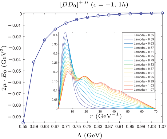
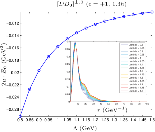
(a)	(b)
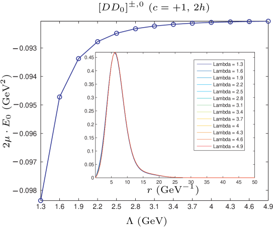
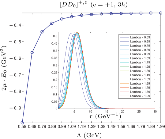
(c)	(d)

Figure 2: The dependence of the binding energy of the $[DD_{0}]^{\pm,0}$ system $(c=+1)$ on $\Lambda$ and the wave function of this system. Here, we only consider the single $\pi$ exchange potential. (a), (b), (c) and (d) correspond to the case of $1h$, $1.3h$, $2h$ and $3h$ with $|h|=0.56$ respectively.

(a)	(b)
(c)	(d)

Figure 20: (a), (b), (c) and (d) are the potentials of the $[D^{*}D_{0}^{*}]_{s1}^{0}$ with $(c=+1,\,\beta\beta^{\prime}>0)$, $(c=+1,\,\beta\beta^{\prime}<0)$, $(c=-1,\,\beta\beta^{\prime}>0)$ and $(c=-1,\,\beta\beta^{\prime}<0)$, respectively. Here, we take $\zeta\varpi>0$ with $|\beta|=0.909$, $|\beta^{\prime}|=0.533$, $|\zeta|=0.727$ and $|\varpi|=0.364$.

References

- (1) S. K. Choi et al., Phys. Rev. Lett. 91, 262001 (2003).
- (2) S. K. Choi et al., Phys. Rev. Lett. 94, 182002 (2005).
- (3) B. Aubert et al., BABAR Collaboration, Phys. Rev. Lett. 95, 142001 (2005).
- (4) C. Z. Yuan et al., Belle Collaboration, Phys. Rev. Lett. 99, 182004 (2007).
- (5) S. Uehara et al., Phys. Rev. Lett. 96, 082003 (2006).
- (6) K. Abe et al., Phys. Rev. Lett. 98, 082001 (2007).
- (7) B. Aubert et al., BABAR Collaboration, Phys. Rev. Lett. 98, 212001 (2007).
- (8) X. L. Wang et al., Belle Collaboration, Phys. Rev. Lett. 99, 142002 (2007).
- (9) S. K. Choi et al., Belle Collaboration, Phys. Rev. Lett. 100, 142001 (2008).
- (10) R. Mizuk et al., Belle Collaboration, Phys. Rev. D 78, 072004 (2008).
- (11) T. Aaltonen et al., CDF Collaboration, Phys. Rev. Lett. 102, 242002 (2009).
- (12) E. S. Swanson, Phys. Lett. B 598, 197 (2004); E. S. Swanson, Phys. Lett. B 588, 189 (2004); T. Fernandez-Carames, A. Valcarce, and J. Vijande, Phys. Rev. Lett. 103, 222001 (2009).
- (13) F. E. Close and C. Downum, Phys. Rev. Lett. 102, 242003 (2009); F. E. Close, C. Downum, and C. E. Thomas, arXiv:1001.2553v1 [hep-ph].
- (14) S. H. Lee, A. Mihara, F. Navarra, and M. Nielsen, Phys. Lett. B 661, 28 (2008); C. Meng and K. T. Chao, arXiv:0708.4222 [hep-ph]; G. J. Ding, arXiv:0711.1485 [hep-ph].
- (15) N. Mahajan Phys. Lett. B 679, 228 (2009); T. Branz, T. Gutsche, and V. E. Lyubovitskij, Phys. Rev. D 80, 054019 (2009); G. J. Ding, Eur. Phys. J. C 64 297 (2009).
- (16) X. Liu, Z. G. Luo, Y. R. Liu, Shi-Lin Zhu, Eur. Phys. J. C 61, 411 (2009), arXiv:0808.0073 [hep-ph].
- (17) Y. R. Liu, X. Liu, W. Z. Deng, Shi-Lin Zhu, Eur. Phys. J. C 56, 63 (2008), arXiv:0801.3540 [hep-ph].
- (18) X. Liu, Y.R. Liu, W. Z Deng, and S. L. Zhu, Phys. Rev. D 77, 094015 (2008).
- (19) X. Liu, Y.R. Liu, W. Z Deng, and S. L. Zhu, Phys. Rev. D 77, 034003 (2008).
- (20) X. Liu and S. L.Zhu, Phys. Rev. D 80, 017502 (2009).
- (21) B. Hu, X.L. Chen, Z.G. Luo, P.Z. Huang, S.L. Zhu, P.F. Yu and X. Liu, arXiv:1004.4032 [hep-ph].
- (22) C. Amsler et al., (Particle Data Group), Phys. Lett. B 667, 1 (2008).
- (23) R. Casalbuoni, A. Deandrea, N. Di Bartolomeo, R. Gatto, F. Feruglio and G. Nardulli, Phys. Rept. 281, 145 (1997) [arXiv:hep-ph/9605342].
- (24) P. Z. Huang, L. Zhang, Shi-Lin Zhu, Phys. Rev. D 80, 014023 (2009).