Multiple hydrodynamical shocks induced by Raman effect in photonic crystal fibres

Abstract

We theoretically predict the occurrence of multiple hydrodynamical-like shock phenomena in the propagation of ultrashort intense pulses in a suitably engineered photonic crystal fiber. The shocks are due to the Raman effect, which acts as a nonlocal term favoring their generation in the focusing regime. It is shown that the problem is mapped to shock formation in the presence of a slope and a gravity-like potential. The signature of multiple shocks in XFROG signals is unveiled.

I Introduction

The existence of regimes where nonlinear optical propagation and Bose-Einstein condensation (BEC) obey hydrodynamical-like models is well known Gurevich and Krylov (1987); Anderson et al. (1992); Stringari (1996); Kodama (1999); Forest et al. (1999). Among the resulting hydrodynamic-like phenomena for intense light pulses or spatial beams, the most fascinating is certainly the formation of shocks Landau and Lifshitz (1995), which can also be considered in Bose-Einstein condensates (BEC) Rothenberg and Grischkowsky (1989); Cai et al. (1997); Ablowitz et al. (2009); Pérez-García et al. (2004); Kamchatnov et al. (2004); Wan et al. (2007); Hoefer et al. (2006); Chang et al. (2008).

Theoretical and experimental work on optical shock formation has been recently reported for nonlocal media, like thermal liquids Ghofraniha et al. (2007); Fratalocchi et al. (2008); Conti et al. (2009), liquid crystals Assanto et al. (2008) and photorefractive materials El et al. (2007); Wan et al. (2010). In the time domain, shocks have been considered in connection with the carrier wave Flesch et al. (1996) and quadratic media Degasperis et al. (2006). Spatiotemporal hyperbolic shocks have also been studied Berge et al. (2002), together with related nonlinear X-wave generation Conti et al. (2003); Bragheri et al. (2007) and multidimensional effects Armaroli et al. (2009); Hoefer and Ilan (2009).

When considering temporal shocks, if it is true that the development of extreme nonlinear optics Brabec and Krausz (2000) unavoidably requires the consideration of ultra-wide spectral-band and intense excitations (common to all shock phenomena), the presence of higher order effects radically affects shock formation and related regularization processes, such as undular bores Whitham (1999); Gurevich and Pitaevskii (1973). In this respect, microstructured photonic-crystal fibers (PCFs) Russell (2003) offer an unprecedented framework for exploring the hydrodynamical properties of light. Indeed, not only do solid-core PCFs exhibit very pronounced nonlinear effects (mainly thanks to their small effective modal areas), but their dispersion profile can be engineered to a large degree. The latter circumstance is particularly appealing for the physics of shock wave generation, because most of the dynamics described by nonlinear Schrödinger (NLS) models predict wave-breaking phenomena in the limit of vanishing dispersion. Such a condition, for temporal shocks, is in general very difficult to achieve over wide spectral regions. PCFs can however be designed with almost flat dispersion over bandwidths of several hundreds nanometers, thus opening up new perspectives in temporal optical shock generation and related applications.

From a theoretical point of view, there are still several open problems concerning the physics of optical shocks. One of the most challenging is the onset of wave-breaking phenomena in the regime of focusing nonlinearity and anomalous group velocity dispersion. Even if unstable kink-antikink solutions (regularized shock fronts without oscillations) are known to exist when including Raman terms Agrawal and Headley (1992); Kivshar and Malomed (1993), the standard hydrodynamical limit of the NLS apparently rules out shock formation in the focusing regime, as the jump condition on the resulting Euler equations (see, e.g, Hoefer et al. (2006)) gives an imaginary result, which does not have a simple physical interpretation. However, it has been shown that, in non-local models Ghofraniha et al. (2007) for spatial beam propagation and BEC, a multi-valued solution of the hydrodynamical equation for the so-called velocity field can be predicted by using the method of characteristics. Such a solution corresponds in the numerical simulations of the nonlocal NLS to the clear formation of an undular-like bore in a regime in which it competes with the modulational instability, as also considered in Assanto et al. (2008). The scenario is hence extremely rich and interesting, and the open question is whether temporal shocks, undular bores and wave-breaking phenomena may form in a focusing regime when considering a real-world system.

The most natural counterpart of a nonlocal nonlinear response in the time domain is the Raman effect. Indeed this is described by a kernel response function, which, under suitable conditions on the pulse duration, leads to a nonlinear shock term containing the first-order derivative of the intensity Agrawal (2007). Previous investigations of intense light propagation in solid-core PCFs when including the Raman effect have shown that the peculiar breathing phenomenon exhibited by higher-order solitons can be used to excite the formation of quasi-symmetric resonant radiation in a step-like fashion in presence of highly distorted GVD Tran and Biancalana (2009). However, in that work, and in all previous observations of the phenomenon (see e.g. Cristiani et al. (2004)), there is no convincing explanation of why the soliton breathing should increase its rate in the presence of the Raman effect, which leads to soliton splitting, and the internal dynamics of the breathing has currently a rather cumbersome interpretation.

In this paper we show that under suitable conditions the soliton breathing process is accompanied by the formation of multiple optical shock waves leading to strong spectral broadening, and that this can described by a hydrodynamical model containing a gravity-like slope term, or equivalently a constant external electric field in a cold plasma. This point of view allows one to clarify and shed new light on the several well-known phenomena described above. Our theoretical results are validated by real-world simulations in a realistic PCF, and represent the first theoretical prediction of shock waves in the focusing regime, also unveiling their measurable signatures in the XFROG signal.

The paper is organized as follows. In section II we discuss the hydrodynamical model for the NLS in the presence of a Raman term. In section III we adopt the method of characteristics to predict and give a mechanical interpretation to the occurrence of multi-valued solutions for the velocity-field. In section IV we describe the PCF we used for investigating temporal hydrodynamic-like shocks and report on the corresponding simulations and the XFROG signal at the shock formation. Conclusions are drawn in section V.

II The hydrodynamical limit in the accelerated reference frame

We start by considering the simplest model for an optical pulse propagating in an optical fibre, described by the envelope equation Agrawal (2007)

$$i\psi_{z}+\frac{1}{2}\psi_{tt}+|\psi|^{2}\psi-\tau_{R}\psi\partial_{t}|\psi|^{2}=0.$$ (1)

In Eq. (1), $\psi$ is the envelope of the electric field, scaled with the soliton power $P_{0}=|\beta_{2}|/(\gamma t_{0})$, where $\beta_{2}$ is the second order dispersion coefficient, $\gamma$ is the nonlinear coefficient of the fiber, and $t_{0}$ is the input pulse duration. The dimensionless propagation length $z$ is scaled with the second order dispersion length $L_{\rm D2}=t_{0}^{2}/|\beta_{2}|$, while the temporal variable $t$ is scaled with $t_{0}$. The last term in (1) represents the Raman effect, and $\tau_{R}\equiv T_{R}/t_{0}$, where $T_{R}$ is the Raman response time (about $2$ fs in silica) Agrawal (2007). For simplicity, only second order dispersion has been included in the model of Eq. (1). Note that Eq. (1) is written in the anomalous dispersion regime, where bright solitons are expected in the absence of the Raman term ($\tau_{R}=0$). Eq. (1) is subject to the initial condition

$$\psi(z=0,t)=N\textrm{sech}\left(t\right).$$ (2)

The generation of the shock-like dynamics corresponds to the case of large $N$, and introducing the smallness parameter $\epsilon\sim 1/\sqrt{N}$, the hydrodynamical limit is obtained via rewriting Eq. (1) in the semiclassical form with the scaled variables $z\rightarrow z/\epsilon^{3}$, $t\rightarrow t/\epsilon^{2}$, $\psi\rightarrow\psi\epsilon$, obtaining

$$i\epsilon\psi_{z}+\frac{\epsilon^{2}}{2}\psi_{tt}+|\psi|^{2}\psi-\frac{\tau_{R}}{\epsilon}\psi\partial_{t}|\psi|^{2}=0\text{.}$$ (3)

The Raman term appears at the relevant order in the hydrodynamical limit for $\tau\sim\epsilon$, which is the condition at which the Raman effect radically alters the shock dynamics, as also confirmed by the simulations reported below.

It is interesting to derive the hydrodynamical limit in the accelerated reference frame where the soliton moves in presence of the Raman effect Gorbach and Skryabin (2007). This is obtained by introducing the variable $\xi=t-\frac{g}{2}z^{2}$ (with $g=32\tau_{R}a^{2}/15$ as in Gorbach and Skryabin (2007)), and performing the Gagnon-Bélanger phase transformation Gagnon and Bélanger (1990)

$$\psi=f(\xi,z)\exp[-i(\frac{g^{2}}{3}z^{3}-gzt+az)],$$ (4)

after which the resulting NLS is written as Akhmediev et al. (1996); Gagnon and Bélanger (1990)

$$if_{z}-g\xi f+af+\frac{1}{2}f_{\xi\xi}+|f|^{2}f-\tau_{R}f\partial_{\xi}|f|^{2}=0$$ (5)

Letting $f=\sqrt{\rho}\exp(i\phi)$, and performing a WKB expansion on Eq. (5), one obtains

$$\rho_{z}+\partial_{\xi}(\rho v)=0$$ (6)

$$\phi_{z}+\frac{1}{2}\phi_{\xi}^{2}=-g\xi+a+\rho-\tau_{R}\partial_{\xi}\rho+\frac{1}{4}\frac{1}{\sqrt{\rho}}\frac{\partial}{\partial\xi}\frac{\rho_{\xi}}{\sqrt{\rho}}$$ (7)

By deriving Eq. (7) with respect to $\xi$, one has (after defining the velocity field $v=\phi_{\xi}$, physically corresponding to the instantaneous frequency inside the pulse)

$$v_{z}+vv_{\xi}=-\partial_{\xi}(U_{QP}+U).$$ (8)

The quantum pressure potential is defined as

$$U_{QP}=-\frac{1}{4}\frac{1}{\sqrt{\rho}}\frac{\partial}{\partial_{\xi}}\frac{\rho_{\xi}}{\sqrt{\rho}},$$ (9)

and the modified ’classical’ potential term is

$$U=g\xi-\rho+\tau_{R}\partial_{\xi}\rho.$$ (10)

Note that potential $U$ in Eq. (10) is exactly the same as the one formerly introduced in Gorbach and Skryabin (2007). The above relations show that the hydrodynamical limit of the NLS with Raman corresponds to fluid motion in an accelerated frame (being $g$ the acceleration) or, equivalently, to a charged plasma in a constant electric field of magnitude $g$.

III Effective particle interpretation

Eq. (8) can be solved before the occurrence of shocks in an approximate way by recalling that the equation for $\rho$ is obtained at a higher order in $\epsilon$, and hence that the initial dynamics is ruled by the velocity field $v$ only. This allows, as a zero-order approximation, to take $\rho(\xi)$ as a fixed profile, e.g. as a sech function denoting the initial pulse profile. Eq. (8) can hence be mapped by the method of characteristics into the system of ordinary differential equations

$$\begin{array}[]{l}\frac{d\xi}{dz}=v\\ \frac{dv}{dz}=-\partial_{\xi}U(\xi)\end{array}$$ (11)

with the initial conditions $\xi=s$ and $v=0$ at $z=0$. The solution for a given $\rho(\xi)$, gives the manifold $(\xi(s,z),v(s,z))$, which for a given $z$ provides a parametric plot of $v$ versus $z$ and allows one to predict the occurrence of hydrodynamical shocks.

Eqs. (11) can be interpreted as the motion of a particle with trajectory $\xi(z)$ in the potential $U$ and can be rewritten as a single Newton-like equation

$$\frac{d^{2}\xi}{dz^{2}}=-\frac{\partial U}{\partial\xi}.$$ (12)

Shocks correspond to the case in which the plot of the trajectory in the space $(\xi,v)$ display a vertical slope, i.e. $d\xi/dv=0$.

This can be geometrically interpreted as follows: various trajectories are generated by varying the particle’s initial position $\xi=s$, see Fig. 1(a), which corresponds to considering the motion of particles in the potential $U$ [shown in Fig. 1(b)] for different values of $\tau_{R}$ which are falling (with initially zero velocity) from position $\xi=s$. A shock, i.e. a multi-valued function $v=v(\xi)$ in the plane $(\xi,v)$ [see Fig. 1(c)] corresponds to the existence of trajectories reaching the same position $\xi$ at the same $z$ with different velocities, i.e. to collisions between particles falling from different initial positions under the effect of $U$.

Given the shape of $U(\xi)$, such collisions specifically involve the particles trapped in a bounded motion, which implies the formation of shocks in a periodic fashion, see also Fig. 1(a) and (c).

As $\tau_{R}$ increases the bounded motion occurs within an increasingly smaller region in $\xi$ [the potential well is reduced, as it is clear from Fig. 1(b)], and it becomes negligible for larger values of $\tau_{R}$. This implies that for increasing $\tau_{R}$, shocks become more frequent (as the corresponding particle collisions), but also that the corresponding discontinuities will be less pronounced. Such a qualitative interpretation, gives a simple picture of what is observed in the simulations discussed below.

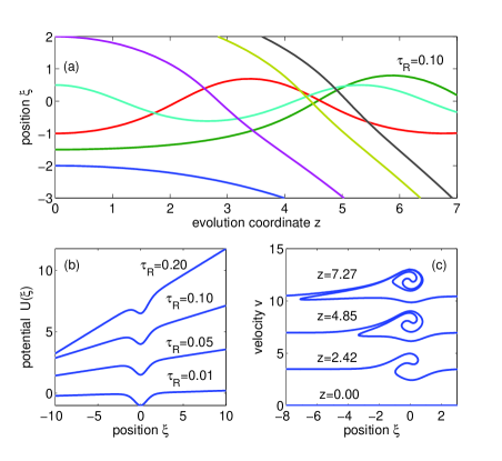
Figure 1: (Color online) (a) Positions of a particle falling inside potential $U(\xi)$ as described by Eq. (10), for different values of the initial position $\xi=s$ and for $\tau_{R}=0.1$. Multiple collisions between oscillating bound particles produce multiple values for the velocity field $v$, i.e. shocks. Non-bound particles can also collide with bound particles – although more rarely – contributing to isolated shocks. (b) Shape of the effective potential for different values of $\tau_{R}$ with $\rho=\textrm{sech}\left(\xi\right)^{2}$; (c) Solution of the hydrodynamical system (11) for different values of $z$, showing multiple-shock occurrences. The velocity is plotted for clarity with an arbitrary vertical shift for the various $z$.

IV Simulations

In this section we show that the hydrodynamical limit of the NLS equation [see Eq. (3)] can be realized in practice through a realistic PCF design. We also compare the simulation dynamics of the idealized model of Eq. (3) with a more realistic simulation based on the full generalized NLS equation (GNLSE).

We start by integrating numerically Eq. (3) with parameters $\tau_{R}=0.1$ and $\epsilon=0.2$, with initial condition $\psi_{\rm in}=\textrm{sech}\left(t\right)$. This set of parameters is chosen to realize the hydrodynamical limit by means of the scaling discussed in section II. After a propagation length of $z\simeq 0.62$, one can observe the formation of the first shock, see Fig. 2(a) where the time-derivative of the phase (i.e. the velocity field) $v(t)\equiv\phi_{t}$ has been plotted. Linked to the formation of the phase shock, one observes the formation of a sharp cusp in the time domain located at the maximum amplitude of the pulse, see Fig. 2(b). Large values of the time-derivative at the cusp produce large spectral broadening in the frequency domain, which in the conventional and very well-known picture is associated with the temporal and spectral ’breathing’ oscillations of higher-order solitons Tran and Biancalana (2009); Agrawal (2007). In the presence of the Raman effect ($\tau_{R}\neq 0$), one will observe the occurrence of multiple shocks, which become more and more frequent during propagation, contrary to the perfectly regular oscillations of the soliton breathing phenomenon in the absence of the Raman Tran and Biancalana (2009); Agrawal (2007). This ’breathing acceleration’ can again be interpreted as multiple shocks of the falling fluid induced by the ’gravity-like’ potential of Eq. (8), as described in section III. Moreover, as is shown in Fig. 2(a), a very clear undular bore phenomenon develops in the trailing edge of the Raman-shifting pulse at longer propagation distances, which does not occur in the absence of the Raman effect. This is associated to the strong oscillations of the velocity field $v$ induced by the quantum pressure potential (9). This term becomes indeed important in proximity of those parts of the pulse for which $\rho\rightarrow 0$, i.e. far from the pulse center. This, when combined with the Raman gravity-like potential (10), leads to the formation and transport of increasingly stronger oscillations in the trailing edge of each pulse.

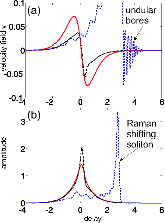
Figure 2: (Color online) Pulse propagation and shock formation according to Eq. (13), using the GVD of Fig. 3. (a) Velocity field $v=\partial_{t}\phi$ as a function of time for three different propagation distances, namely $z=0.4$ (red solid line, before the occurrence of shock), $z=0.62$ (black dotted line, at the moment of shock) and $z=1.5$ (blue dashed line, long distance dynamics), for $\tau_{R}=0.1$ and $\epsilon=0.2$. For long propagation dynamics, the formation of clear undular bores is observed. (b) Amplitude $|\psi|$ at the same values of $z$ as in (a). At the moment of the first shock, a sharp cusp is formed.

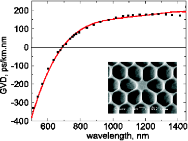
Figure 3: (Color online) GVD curve of the PCF used in our simulations. The black dots represent the data measured experimentally through white-light interferometry, while the solid curve is a polynomial fit. The ZDW is close to $\lambda_{Z}=690$ nm. The inset shows an SEM of the fiber cross section.

We now compare the shock dynamics of the above simplified model with the full GNLSE, applied to a realistic waveguide. In Fig. 3 we show the GVD of a solid-core PCF, the SEM picture of which is given in the inset. The black dots correspond to measured data, while the red solid line shows a fit. The fiber has a core diameter of approximately $1.5$ $\mu$m, an estimated nonlinear coefficient $\gamma\simeq 100$ W^-1m^-1, and a zero-GVD point located at $\lambda_{Z}\simeq 690$ nm. We use the following GNLSE Agrawal (2007):

$$\small{i\partial_{z}\psi+\hat{D}(i\partial_{t})\psi+\left(1+\frac{i\partial_{t}}{\omega_{0}t_{0}}\right)\left[\psi\int_{-\infty}^{+\infty}r(t-t^{\prime})|\psi(t^{\prime})|^{2}dt^{\prime}\right]=0},$$ (13)

where $r(t)=[(1-\theta)\delta(t)+\theta h(t)]/t_{0}$ is the total response function, $t_{0}$ is the input pulse duration, $\theta$ is the relative contribution between the non-instantaneous Raman and the instantaneous Kerr effect in the material ($\theta=0.18$ in silica), $\delta(t)$ is the Dirac-delta function. The Raman response function is introduced in the code by using the Hollenbeck and Cantrell approach Hollenbeck and Cantrell (2002). The $h$-function is normalized, $\int_{-\infty}^{+\infty}r(t^{\prime})dt^{\prime}=1$, while the dimensionless Raman response time parameter used in Eq. (1) and Eq. (3), proportional to the first momentum, is given by $\tau_{R}=(1/t_{0})\int_{-\infty}^{+\infty}t^{\prime}r(t^{\prime})dt^{\prime}$. Operator $\hat{D}(i\partial_{t})$ in Eq. (13) describes the full complexity of the fiber GVD shown in Fig. 3, and is given by $\hat{D}(i\partial_{t})\equiv\sum_{m\geq 2}\frac{\beta_{m}(i\partial_{t})^{m}}{m!}$, where $\beta_{m}\equiv(\partial^{m}\beta(\omega)/\partial\omega^{m})_{\omega=\omega_{0}}$ is the $m$-th derivative of the propagation constant $\beta(\omega)$ calculated at a suitable arbitrary reference frequency $\omega_{0}$.

Figure 4: (Color online) XFROG spectrograms for the pulses at $z$ equal to (a) $1.761$, (b) $2.192$, (c) $2.723$, and (d) $3.393$ cm. The peak power of the $t_{0}=130$ fs input pulse was $P=5$ kW ($N=3.1$), and they were launched at $\lambda=1$ $\mu$m. Fig (a) and (b) are snapshots of the first shock. Fig (c) and (d) show the second shock, coinciding with the second spectral oscillation.

The panels in Fig. 4(a-d) show the evolution of the XFROG trace $I(\delta,\tau)=\left|A(t)A_{\rm ref}(t-\tau)e^{-i\delta t}dt\right|^{2}$ Agrawal (2007) ($A_{\rm ref}$ is a suitable reference pulse) recorded at four different propagation distances, corresponding to the first two occurrences of maximum spectral broadening, for $\lambda=1$ $\mu$m, relatively far from the zero GVD point.

The goal of our simulations is to identify the multiple shock generation during pulse propagation in a PCF. In section II we showed that the hydrodynamical limit requires large N, thus very high peak powers. We find however, that in our siumlations the dynamics of the multiple shock can best be demonstrated for lower N. In this case, the dynamics are not obscured by unwanted effects like resonant radiation, which disturb the soliton propagation and prevents thus a clear signature of the multiple shocks. In this regard, the presented GVD curve in Fig. 3 will be advanteous for the purpose of observing shock phenomena. A higher value of $\beta_{2}$ would lead to a massive Raman self-frequency shift which would obscure shock formation. On the other hand, smaller values of $\beta_{2}$ (or too large values of $N$) lead to a dominating self-phase modulation, since $L_{\rm D2}$ would be much longer that the nonlinear length $L_{\rm NL}=(\gamma P)^{-1}$. In that case, a very strong spectral broadening would be accompanied by the emission of resonant radiation from solitons Biancalana et al. (2004), which would also disturb the formation of clear shocks. The fiber is pumped by a sech pulse with $N=3.1$. The amplitude shocks that develop at these moments are evident. The panels in Fig. 5(a-d) show the corresponding intensity profiles and the velocity field $v(t)=\partial_{t}\phi$ at the same values of $z$ as in Fig. 4. Again, one can see phase discontinuities located at the various pulse centers. Moreover, one can notice the generation of strong undular bores in the trailing edge of the pulse, which agree qualitatively with the simplified model examined above.

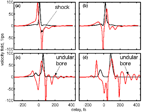
Figure 5: (Color online) (a-d) Amplitude (black dotted line) and velocity field (red solid line) in the same conditions as in Figs. 4(a-d). (a) is the moment of the first shock, while (b-d) show the generation of undular bores from the strong velocity field oscillations of the singularities due to the quantum pressure potential (9).

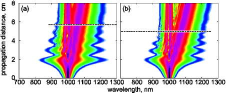
Figure 6: (Color online) Spectral evolution of $P=5$ kW pulses for Raman fractions (a) $f_{R}=0.18$ ($\tau_{R}=0.0334$), and (b) $f_{R}=0.3$ ($\tau_{R}=0.0557$), with $t_{0}=130$ fs and a pulse launched at $\lambda=800$ nm in the PCF of Fig. 3. For increasing values of $\tau_{R}$, the spectral oscillation rate rises, which can be interpreted by the hydrodynamical formulation of Eqs. (6-7). Horizontal dashed lines indicate the distance at which one has 5 spectral oscillations, to help visualization.

In Figs. 6(a,b) we show the evolution of Eq. (13) in two different cases, one for $\tau_{R}=0.0334$ [Fig. 6(a)] and the other for $\tau_{R}=0.0557$ [Fig. 6(b)]. One can notice the well-known slight increase of the rate of spectral oscillations when increasing the value of $\tau_{R}$, which cannot find an easy explanation in the model of Eq. (13). However, such behavior can easily be explained in terms of the hydrodynamical analogy expressed by Eqs. (6-7): in presence of Raman effect, the ’falling’ photon fluid feels a gravity-like field which increases the rate of shocks during propagation, according to the qualitative explanation based on colliding particles given in section III.

V Conclusions

In conclusion we have shown that suitably engineered photonic crystal fibers may sustain the formation of multiple hydrodynamical-like shocks during the propagation of ultrashort pulses. The shocks are shown to be clearly evident in the XFROG signal, have measurable signatures, and occur for a focusing nonlinearity. This effect can be exploited for the optimization and control of supercontinuum generation, and is expected to play a role when considering multidimensional dynamics.

VI Acknowledgements

We acknowledge support from the INFM-CINECA initiative for parallel computing and CASPUR. The research leading to these results has received funding from the European Research Council under the European Community Seventh Framework Program (FP7/2007-2013)/ERC grant agreement n.201766. FB, SS and PSJR are supported by the Max Planck Society for the Advancement of Science (MPG).

References

- Gurevich and Krylov (1987) A. V. Gurevich and A. L. Krylov, Sov. Phys. JETP 65, 994 (1987).
- Anderson et al. (1992) D. Anderson, M. Desaix, M. Lisak, and M. L. Quiroga-Teixeiro, J. Opt. Soc. Am. B 9, 1358 (1992).
- Stringari (1996) S. Stringari, Phys. Rev. Lett. 77, 2360 (1996).
- Kodama (1999) Y. Kodama, SIAM J. Appl. Math. 59, 2162 (1999).
- Forest et al. (1999) M. G. Forest, J. N. Kutz, and K. T. R. McLaughlin, J. Opt. Soc. Am. B p. 1856 (1999).
- Landau and Lifshitz (1995) L. D. Landau and E. M. Lifshitz, Fluid Mechanics (Pergamon, 1995).
- Rothenberg and Grischkowsky (1989) J. E. Rothenberg and D. Grischkowsky, Phys. Rev. Lett. 62, 531 (1989).
- Cai et al. (1997) D. Cai, A. R. Bishop, N. Grønbech-Jensen, and B. A. Malomed, Phys. Rev. Lett. 78, 223 (1997).
- Ablowitz et al. (2009) M. J. Ablowitz, D. E. Baldwin, and M. A. Hoefer, Phys. Rev. E 80, 016603 (2009).
- Pérez-García et al. (2004) V. M. Pérez-García, V. V. Konotop, and V. A. Brazhnyi, Phys. Rev. Lett. 92, 220403 (2004).
- Kamchatnov et al. (2004) A. M. Kamchatnov, A. Gammal, and R. A. Kraenkel, Phys. Rev. A 69, 063605 (2004).
- Wan et al. (2007) W. Wan, S. Jia, and J. W. Fleischer, Nature Phys. 3, 46 (2007).
- Hoefer et al. (2006) M. A. Hoefer, M. J. Ablowitz, I. Coddington, E. A. Cornell, P. Engels, and V. Schweikhard, Phys. Rev. A 74, 023623 (2006).
- Chang et al. (2008) J. J. Chang, P. Engels, and M. A. Hoefer, Phys. Rev. Lett. 101, 170404 (2008).
- Ghofraniha et al. (2007) N. Ghofraniha, C. Conti, G. Ruocco, and S. Trillo, Phys. Rev. Lett. 99, 043903 (2007).
- Fratalocchi et al. (2008) A. Fratalocchi, C. Conti, G. Ruocco, and S. Trillo, Phys. Rev. Lett. 101, 044101 (2008).
- Conti et al. (2009) C. Conti, A. Fratalocchi, M. Peccianti, G. Ruocco, and S. Trillo, Phys. Rev. Lett. 102, 083902 (2009).
- Assanto et al. (2008) G. Assanto, T. R. Marchant, and N. F. Smyth, Phys. Rev. A 78, 063808 (2008).
- El et al. (2007) G. A. El, A. Gammal, E. G. Khamis, R. A. Kraenkel, and A. M. Kamchatnov, Phys. Rev. A 76, 053813 (2007).
- Wan et al. (2010) W. Wan, S. Muenzel, and J. W. Fleischer, Phys. Rev. Lett. 104, 073903 (2010).
- Flesch et al. (1996) R. G. Flesch, A. Pushkarev, and J. V. Moloney, Phys. Rev. Lett. 76, 2488 (1996).
- Degasperis et al. (2006) A. Degasperis, M. Conforti, F. Baronio, and S. Wabnitz, Phys. Rev. Lett. 97, 093901 (2006).
- Berge et al. (2002) L. Berge, K. Germaschewski, R. Grauer, and J. J. Rasmussen, Phys. Rev. Lett. (2002).
- Conti et al. (2003) C. Conti, S. Trillo, P. Di Trapani, G. Valiulis, A. Piskarskas, O. Jedrkiewicz, and J. Trull, Phys. Rev. Lett. 90, 170406 (2003).
- Bragheri et al. (2007) F. Bragheri, D. Faccio, A. Couairon, A. Matijosius, G. Tamošauskas, A. Varanaviius, V. Degiorgio, A. Piskarskas, and P. Di Trapani, Phys. Rev. A 76, 025801 (2007).
- Armaroli et al. (2009) A. Armaroli, S. Trillo, and A. Fratalocchi, Phys. Rev. A 80, 053803 (2009).
- Hoefer and Ilan (2009) M. A. Hoefer and B. Ilan, Phys. Rev. A 80, 061601 (2009).
- Brabec and Krausz (2000) T. Brabec and F. Krausz, Rev. Mod. Phys. 72, 545 (2000).
- Whitham (1999) G. B. Whitham, Linear and Nonlinear Waves (Wiley, New York, 1999).
- Gurevich and Pitaevskii (1973) A. V. Gurevich and L. Pitaevskii, Sov. Phys. JETP 38, 291 (1973).
- Russell (2003) P. S. J. Russell, Science 299, 358 (2003).
- Agrawal and Headley (1992) G. P. Agrawal and C. Headley, Phys. Rev. A 46, 1573 (1992).
- Kivshar and Malomed (1993) Y. S. Kivshar and B. A. Malomed, Opt. Lett. 18, 485 (1993).
- Agrawal (2007) G. P. Agrawal, Nonliner Fibre Optics (Academic Press, San Diego, 2007), 4th ed.
- Tran and Biancalana (2009) T. X. Tran and F. Biancalana, Phys. Rev. A 79, 065802 (2009).
- Cristiani et al. (2004) I. Cristiani, R. Tediosi, L. Tartara, and V. Degiorgio, Opt. Expr. 12, 124 (2004).
- Gorbach and Skryabin (2007) A. V. Gorbach and D. V. Skryabin, Phys. Rev. A 76, 053803 (2007).
- Gagnon and Bélanger (1990) L. Gagnon and P. A. Bélanger, Opt. Lett. 15, 466 (1990).
- Akhmediev et al. (1996) N. Akhmediev, W. Królikovski, and A. Lowery, Opt. Commun. 131, 260 (1996).
- Hollenbeck and Cantrell (2002) D. Hollenbeck and C. D. Cantrell, J. Opt. Soc. Am. B 19, 2886 (2002).
- Biancalana et al. (2004) F. Biancalana, D. V. Skryabin, and A. V. Yulin, Phys. Rev. E 70, 016615 (2004).