Average phase factor in the PNJL model

Abstract

The average phase factor $\langle e^{2i\theta}\rangle$ of the QCD determinant is evaluated at finite quark chemical potential ($\mu_{\rm q}$) with the two-flavor version of the Polyakov-loop extended Nambu-Jona-Lasinio (PNJL) model with the scalar-type eight-quark interaction. For $\mu_{\rm q}$ larger than half the pion mass $m_{\pi}$ at vacuum, $\langle e^{2i\theta}\rangle$ is finite only when the Polyakov loop is larger than $\sim 0.5$, indicating that lattice QCD is feasible only in the deconfinement phase. A critical endpoint (CEP) lies in the region of $\langle e^{2i\theta}\rangle=0$. The scalar-type eight-quark interaction makes it shorter a relative distance of the CEP to the boundary of the region. For $\mu_{\rm q}<m_{\pi}/2$, the PNJL model with dynamical mesonic fluctuations can reproduce lattice QCD data below the critical temperature.

I Introduction

The thermodynamics of quantum chromodynamics (QCD) is well defined, since QCD is renormalizable and parameter free. Nevertheless, the thermodynamics is not understood at lower temperature ($T$) because of its nonperturbative nature. The thermodynamics is closely related to not only natural phenomena such as compact stars and the early universe but also laboratory experiments such as relativistic heavy-ion collisions. Lattice QCD (LQCD) is a first-principle calculation, but it has the well-known sign problem when the quark-number chemical potential ($\mu_{\rm q}$) is real; for example, see Ref. Kogut (2007). So far, several approaches have been proposed to circumvent the difficulty; for example, the reweighting method Fodor (2002), the Taylor expansion method Allton (2004) and the analytic continuation from imaginary $\mu_{\rm q}$ to real $\mu_{\rm q}$ Forcrand and Philipsen (2002); Elia and Lombardo (2003, 2003); Chen and Luo (2005). However, these are still far from perfection particularly at $\mu_{\rm q}/T\mathrel{\mathchoice{\lower 3.6pt\vbox{\halign{$\mathsurround=0pt\displaystyle\hfil#\hfil$\cr>\crcr\sim\crcr}}}{\lower 3.6pt\vbox{\halign{$\mathsurround=0pt\textstyle\hfil#\hfil$\cr>\crcr\sim\crcr}}}{\lower 3.6pt\vbox{\halign{$\mathsurround=0pt\scriptstyle\hfil#\hfil$\cr>\crcr\sim\crcr}}}{\lower 3.6pt\vbox{\halign{$\mathsurround=0pt\scriptscriptstyle\hfil#\hfil$\cr>\crcr\sim\crcr}}}}1$.

The success of the approaches is linked to how difficult the sign problem is. As a good index of the difficulty, one can consider the average of the phase factor

$$e^{2i\theta}=\frac{\det(D+\mu_{\rm q}\gamma_{0}+m)}{\det(D+\mu_{\rm q}\gamma_{0}+m)^{*}}$$ (1)

of the Fermion determinant. If the average of the phase factor is much smaller than 1, this means that there are severe cancellations in the path integral of the QCD partition function. In this situation, LQCD simulations are not feasible.

The average is obtained by taking the expectation value of the phase factor in the phase-quenched theory in which the Fermion determinant is replaced by the absolute value. In the two-flavor case, the average is

$$\langle e^{2i\theta}\rangle=\frac{Z_{1+1}}{Z_{1+1^{*}}},$$ (2)

where $Z_{1+1}$ stands for the partition function of the ordinary two-flavor theory and $Z_{1+1^{*}}$ represents that of the two-flavor phase-quenched theory in which one of two flavors is changed into a conjugate flavor. For comparison of the 1+1^∗ system with the 1+1 system, let us introduce the modified isospin chemical potential $\mu_{\rm I}$ related to the isospin chemical potential $\mu_{\rm iso}$ as $\mu_{\rm I}=\mu_{\rm iso}/2$. When the 1+1 system has a value of $\mu_{q}$, the 1+1^∗ system possesses the same value of $\mu_{\rm I}$.

It is not easy to calculate the average phase factor with LQCD even for small $\mu_{\rm q}/T$. Actually, several LQCD results on the average phase factor are spotted; see Ref. Han and Stephanov (2008) and references therein. It is then important to make a systematic analysis on the phase factor by using effective theories. This was done by the chiral perturbation theory Splittorff and Verbaarschot (2007); Bloch and Wettig (2008). The result is consistent with LQCD one Han and Stephanov (2008) when $T$ is lower than the critical one $T_{\rm c}$. However, the theory is not valid for $T>T_{\rm c}$.

Recently, the average phase factor at $T>T_{\rm c}$ was calculated by the random matrix theory Han and Stephanov (2008) and the Nambu–Jona-Lasinio (NJL) model Anderson et al. (2010). When the saddle-point approximation is applied to the path integrals in the partition functions $Z_{1+1}$ and $Z_{1+1^{*}}$, the average phase factor can be described by

$$\langle e^{2i\theta}\rangle\approx\frac{\sqrt{\det H_{1+1^{*}}}}{\sqrt{\det H_{1+1}}}e^{-\beta V(\Omega_{1+1}-\Omega_{1+1^{*}})},$$ (3)

where $\beta=1/T$, $\Omega$ is the thermodynamic potential at mean field level and $H$ is the Hessian matrix showing static fluctuations (SF) at the saddle point. The average phase factor thus obtained is dominated not by the exponential factor $e^{-\beta V(\Omega_{1+1}-\Omega_{1+1^{*}})}$ but by the SF factor ${\sqrt{\det H_{1+1^{*}}}}/{\sqrt{\det H_{1+1}}}$ Anderson et al. (2010), because $\Omega_{1+1}=\Omega_{1+1^{*}}$ in the normal phase with no pion condensate and the SF factor is zero in the pion condensate phase; this will be explained explicitly in subsection II.2. Thus, the average phase factor should be calculated with the mean field (MF) approximation plus SF corrections. This framework is referred to as MF+SF in the present paper.

The NJL model describes the chiral phase transition  Nambu and Jona-Lasinio (1961a); Asakawa and Yazaki (1989); S. P. Klevansky (1992); Hatsuda and Kunihiro (1994); Kashiwa et al (2006, 2006), but not the deconfinement transition. The Polyakov-loop extended Nambu–Jona-Lasinio (PNJL) model Meisinger et al. (1996); Fukushima (2004, 2008); S. K. Ghosh et al. (2006); Megias et al. (2006); Ratti et al. (2006); Rossner et al. (2007); Ciminale (2007); Schaefer (2007); Zhang et al (2007); Mukherjee et al (2007); Costa et al (2008); Kashiwa et al (2008); Fu (2007); Hell et al (2009); Sakai et al (2008, 2009); Sakai (2009); Xiong (2009); Sasaki et al. (2009) was constructed to treat both the transitions simultaneously. Very recently, the PNJL model was shown to be successful in reproducing LQCD data for imaginary quark chemical potential Sakai et al (2008, 2009), imaginary quark and isospin chemical potentials Sakai (2009) and real isospin chemical potential Sasaki et al. (2009). Thus, the PNJL model is one of the most reliable models.

In this paper, we evaluate the average phase factor by the PNJL model in the MF+SF framework and investigate a relation between the Polyakov-loop and the average phase factor. For thermal systems at $\mu_{\rm I}=\mu_{\rm q}=0$ and at $\mu_{\rm I}>0$ and $\mu_{\rm q}=0$, the scalar-type eight-quark interaction is essential for the PNJL model to reproduce LQCD data Sakai et al (2009); Sasaki et al. (2009). We then analyze an effect of the eight-quark interaction on the average phase factor, too. Finally, we consider dynamical mesonic fluctuations (DF), instead of static mesonic fluctuations, to compare the PNJL results with LQCD data.

This paper is organized as follows. In Sec. II, we recapitulate the PNJL model and a way of calculating the average phase factor. The numerical results are shown in Sec. III. Effects of the Polyakov loop, the eight-quark interaction, static fluctuations and dynamical mesonic fluctuations are investigated. Section IV is devoted to summary.

II Formalism

In this section, we first explain the PNJL model in the MF level for the case of finite $\mu_{\rm q}$ and $\mu_{\rm I}$ and treat SF in order to evaluate the average phase factor.

II.1 PNJL model

The Lagrangian of the two-flavor PNJL model in Euclidean spacetime is

$$\mathcal{L} = \bar{q}(\gamma_{\nu}D^{\nu}-\gamma_{4}{\hat{\mu}}+{\hat{m}}_{0})q+G_{\rm s}\left[(\bar{q}q)^{2}+(\bar{q}i\gamma_{5}\vec{\tau}q)^{2}\right]$$

$$+ G_{\rm s8}\left[(\bar{q}q)^{2}+(\bar{q}i\gamma_{5}\vec{\tau}q)^{2}\right]^{2}-{\cal U}(\Phi[A],{\Phi}[A]^{*},T),$$ (4)

where $D^{\nu}=\partial^{\nu}+iA^{\nu}$ and $A^{\nu}=\delta^{\nu}_{0}gA^{0}_{a}{\lambda^{a}\over{2}}$ with the gauge field $A^{\nu}_{a}$, the Gell-Mann matrix $\lambda_{a}$ and the gauge coupling $g$. The coupling constant $G_{\rm s}$ ($G_{\rm s8}$) represents a strength of the scalar-type four-quark (eight-quark) interaction. The Polyakov potential ${\cal U}$ of (20) is a function of the Polyakov loop $\Phi$ and its Hermitian conjugate $\Phi^{*}$.

The chemical potential matrix ${\hat{\mu}}$ is defined by ${\hat{\mu}}={\rm diag}(\mu_{u},\mu_{d})$ with the $u$-quark ($d$-quark) number chemical potential $\mu_{u}$ ($\mu_{d}$), while ${\hat{m}}_{0}={\rm diag}(m_{0},m_{0})$. The chemical potential matrix is described by $\mu_{\rm q}$ and $\mu_{\rm I}$ as

$${\hat{\mu}}=\mu_{\rm q}\tau_{0}+\mu_{\rm I}\tau_{3},$$ (5)

where $\tau_{0}$ is the unit matrix and $\tau_{i}$ ($i=1,2,3$) are the Pauli matrices in flavor space. The $\mu_{\rm q}$ and $\mu_{\rm I}$ are related to the baryon and isospin chemical potentials, $\mu_{\rm B}$ and $\mu_{\rm iso}$, coupled respectively to the baryon charge ${\bar{B}}$ and to the isospin charge ${\bar{I}_{3}}$ as

$$\mu_{\rm q}=\frac{\mu_{u}+\mu_{d}}{2}=\frac{\mu_{\rm B}}{3},~{}~{}\mu_{\rm I}=\frac{\mu_{u}-\mu_{d}}{2}=\frac{\mu_{\rm iso}}{2}.$$ (6)

For later convenience, we use $\mu_{\rm I}$ instead of $\mu_{\rm iso}$ and call it the isospin chemical potential simply. The $1$+$1$ and the $1$+$1^{*}$ theory correspond to taking $(\mu_{\rm q},\mu_{\rm I})=(\mu_{\rm q},0)$ and $(0,\mu_{\rm q})$, respectively, in $\mathcal{L}$ of (4). In the limit of $m_{0}=\mu_{\rm I}=0$, the PNJL Lagrangian has the $SU_{\rm L}(2)\times SU_{\rm R}(2)\times U_{\rm v}(1)\times SU_{\rm c}(3)$ symmetry. For $m_{0}\neq 0$ and $\mu_{\rm I}\neq 0$, it is reduced to $U_{\rm I_{3}}(1)\times U_{\rm v}(1)\times SU_{\rm c}(3)$.

The Polyakov-loop operator $\hat{\Phi}$ and its Hermitian conjugate $\hat{\Phi}^{\dagger}$ are defined as

$$\hat{\Phi} = {1\over 3}{\rm Tr}L,~{}~{}~{}~{}\hat{\Phi}^{*}={1\over 3}{\rm Tr}L^{\dagger},$$ (7)

with

$$L({\bf x}) = {\cal P}\exp\Bigl{[}{i\int^{\beta}_{0}d\tau A_{4}({\bf x},\tau)}\Bigr{]},$$ (8)

where ${\cal P}$ is the path ordering and $A_{4}=iA^{0}$. In the Polyakov gauge, $L$ can be written in a diagonal form in color space Fukushima (2004):

$$L=e^{i\beta(\phi_{3}\lambda_{3}+\phi_{8}\lambda_{8})}.$$ (9)

In the MF level, $\phi_{3}$ and $\phi_{8}$ are treated as classical variables Rossner et al. (2007).

The spontaneous breakings of the chiral and the $U_{\rm I_{3}}(1)$ symmetry are described, respectively, by the chiral condensate $\sigma=\langle\bar{q}q\rangle$ and the charged pion condensate Zhang et al (2007)

$$\pi^{\pm}=\frac{\pi}{\sqrt{2}}e^{\pm i\alpha}=\langle\bar{q}i\gamma_{5}\tau_{\pm}q\rangle.$$ (10)

Since the phase $\alpha$ represents the direction of the $U_{\rm I_{3}}(1)$ symmetry breaking, we take $\alpha=0$ for convenience. The pion condensate is then expressed by

$$\pi=\langle\bar{q}i\gamma_{5}\tau_{1}q\rangle.$$ (11)

Making the MF approximation Kashiwa et al (2006); Zhang et al (2007), one can obtain the MF Lagrangian as

$${\cal L}_{\rm MF} = {\bar{q}}(\gamma_{\nu}D^{\nu}-\gamma_{4}{\hat{\mu}}+M\tau_{0}+Ni\gamma_{5}\tau_{1})q~{}~{}~{}~{}~{}~{}$$

$$+G_{\rm s}[\sigma^{2}+\pi^{2}]+3G_{\rm s8}(\sigma^{2}+\pi^{2})^{2}+{\cal U}\quad$$ (12)

with

$$M = m_{0}-2[G_{\rm s}+2G_{\rm s8}(\sigma^{2}+\pi^{2})]\sigma,~{}~{}$$

$$N = -2[G_{\rm s}+2G_{\rm s8}(\sigma^{2}+\pi^{2})]\pi.$$ (13)

The quark propagator ${\cal S}$ in the MF level, that has off-diagonal elements in flavor space, is obtained by

$${\cal S}^{-1}(p)=\left(\begin{array}[]{cc}\gamma_{\nu}P^{\nu}-\mu_{u}\gamma_{4}+M&-i\gamma_{5}N\\ i\gamma_{5}N&\gamma_{\nu}P^{\nu}-\mu_{d}\gamma_{4}+M\end{array}\right),$$ (16)

where $P^{\nu}=p^{\nu}-A^{\nu}$. Performing the path integral in the PNJL partition function

$$Z_{\rm MF}=\int DqD\bar{q}\exp\left[-\int d^{4}x{\cal L}_{\rm MF}\right],$$ (17)

we can get the thermodynamic potential (per unit volume),

$$\Omega_{\rm MF} =-T\ln(Z_{\rm MF})/V=-2\sum_{i=\pm}\int\frac{d^{3}{\rm p}}{(2\pi)^{3}}\Bigl{[}3E_{i}({\rm p})$$

$$+\frac{1}{\beta}\ln~{}[1+3(\Phi+\Phi^{*}e^{-\beta E_{i}^{-}({\bf p})})e^{-\beta E_{i}^{-}({\bf p})}+e^{-3\beta E_{i}^{-}({\bf p})}]$$

$$+\frac{1}{\beta}\ln~{}[1+3(\Phi^{*}+{\Phi e^{-\beta E_{i}^{+}({\bf p})}})e^{-\beta E_{i}^{+}({\bf p})}+e^{-3\beta E_{i}^{+}({\bf p})}]\Bigl{]}$$

$$+G_{\rm s}[\sigma^{2}+\pi^{2}]+3G_{\rm s8}(\sigma^{2}+\pi^{2})^{2}+{\cal U}$$ (18)

with

$$E_{\pm}^{\pm}({\rm p})=E_{\pm}({\rm p})\pm\mu_{\rm q},$$ (19)

where $E_{\pm}({\rm p})=\sqrt{(E({\rm p})\pm\mu_{\rm I})^{2}+N^{2}}$ and $E({\rm p})=\sqrt{{\bf p}^{2}+M^{2}}$. The mometum integral in (18) is regularized by the three-dimensional cutoff $\Lambda$.

We use ${\cal U}$ of Ref. Rossner et al. (2007):

$${\cal U}=T^{4}\Bigl{[}-\frac{a(T)}{2}{\Phi}^{*}\Phi$$

$$~{}~{}~{}~{}~{}+b(T)\ln(1-6{\Phi\Phi^{*}}+4(\Phi^{3}+{\Phi^{*}}^{3})-3(\Phi\Phi^{*})^{2})\Bigr{]},$$ (20)

$$a(T)=a_{0}+a_{1}\Bigl{(}\frac{T_{0}}{T}\Bigr{)}+a_{2}\Bigl{(}\frac{T_{0}}{T}\Bigr{)}^{2},~{}~{}~{}b(T)=b_{3}\Bigl{(}\frac{T_{0}}{T}\Bigr{)}^{3}.$$ (21)

The parameters of ${\cal U}$ are adjusted to LQCD data in the heavy-quark (pure-gauge) limit Boyd et al. (1996); Kaczmarek (2002); the resultant parameter set is shown in Table I. In the limit, the Polyakov potential yields a first-order deconfinement phase transition at $T=T_{0}$. Since the first-order transition takes place at $T=270$ MeV in LQCD, $T_{0}$ is often set to 270 MeV in the PNJL calculation. In the light-quark case, however, the PNJL calculation with this value of $T_{0}$ yields a larger value of $T_{\mathrm{c}}$ than the full LQCD prediction $T_{\mathrm{c}}=173$ MeV Karsch (2002); Karsch, Leermann and Peikert (2002); Kaczmarek2 . Therefore, we rescale $T_{0}$ to 200 MeV to reproduce $T_{\mathrm{c}}=173$ MeV Sakai et al (2009).

$a_{0}$	$a_{1}$	$a_{2}$	$b_{3}$
3.51	-2.47	15.2	-1.75

Table 1: Summary of the parameter set in the Polyakov-potential sector determined in Ref. Rossner et al. (2007). All parameters are dimensionless.

In the NJL sector, two parameter sets are taken; in the first set $G_{\rm s8}$ is finite, while in the second set it is zero. The first set is $\Lambda=0.6315$ GeV, $G_{\rm s}=4.673$ [GeV${}^{-2}]$, $G_{\rm s8}=452.12$ [GeV${}^{-8}]$ and $m_{0}=5.5$ MeV. This set reproduces not only the pion decay constant $f_{\pi}=93.3$ MeV and the pion mass $m_{\pi}=139$ MeV at vacuum but also LQCD data Karsch, Leermann and Peikert (2002); Karsch (2002); Kaczmarek2 on $\sigma$ and $|\Phi|$ for thermal systems with no $\mu_{\rm q}$ and $\mu_{\rm I}$ Sakai et al (2009). The second set is $\Lambda=0.6315$ GeV, $G_{\rm s}=5.498$ GeV^-2, $G_{\rm s8}=0$ and $m_{0}=5.5$ MeV. This set can reproduce the pion decay constant and the pion mass at vacuum, but not LQCD data for thermal systems with no $\mu_{\rm q}$ and $\mu_{\rm I}$. Thus, the first set with finite $G_{\rm s8}$ is more reliable.

II.2 Average phase factor

As mentioned in section I, we have to consider fluctuations to mean fields to evaluate the average phase factor. In this subsection, we consider static fluctuations (SF).

In the path-integral representation of the partition function $Z$ or the thermodynamic potential $\Omega$, $\phi_{3}$ and $\phi_{8}$ are fundamental fields rather than $\Phi$ and $\Phi^{*}$. This means that we should solve the stationary conditions

$$\frac{\partial\Omega}{\partial\varphi}=0$$ (22)

for $\varphi=(\sigma,\vec{\pi},\phi_{3},\phi_{8})$ rather than $\varphi=(\sigma,\vec{\pi},\Phi,\Phi^{*})$ Rossner et al. (2007), although the solutions are not so different between the two cases. However, the first case does not guarantee that $\Omega$ is real. Following Ref. Rossner et al. (2007), we then put $\phi_{8}=0$ to keep $\Omega$ real. Noting that the first-order derivative with respect to $\phi_{8}$ does not vanish, we expand $\Omega$ up to quadratic terms of fluctuations:

$$\Omega=\Omega_{\rm MF}+\left(\frac{\delta\Omega}{\delta\varphi_{i}}\right)_{\rm MF}\delta\varphi_{i}+\frac{1}{2}\left(\frac{\delta^{2}\Omega}{\delta\varphi_{i}\delta\varphi_{j}}\right)_{\rm MF}\delta\varphi_{i}\delta\varphi_{j},~{}~{}~{}$$ (23)

where $\varphi=\sum_{i}\delta\varphi_{i}+\varphi_{\rm MF}$ for mean fields $\varphi_{\rm MF}$ and static (constant) fluctuations $\delta\varphi_{i}$. Since first-order terms in $\delta\varphi_{i}$ are purely imaginary, we can regard an integral over $\delta\varphi_{i}$ as a Fourier integral. We then obtain

$$Z = \int\prod_{i}d(\delta\varphi_{i})\exp\left[-\frac{V}{T}\Omega\right]=\frac{1}{\cal N}\exp\left[-\frac{V}{T}\tilde{\Omega}\right]~{}~{}~{}~{}~{}~{}~{}$$ (24)

with

$$\tilde{\Omega}=\left\{\Omega_{\rm MF}+\frac{1}{2}\left(\frac{\delta^{2}\Omega}{\delta^{2}\phi_{8}}\right)^{-1}_{\rm MF}\left(\frac{\delta\Omega}{\delta\phi_{8}}\right)^{2}_{\rm MF}\right\}$$ (25)

and

$${\cal N}=\left(\frac{V}{2\pi T}\right)^{\frac{n}{2}}\left\|\det H\right\|^{\frac{1}{2}},~{}~{}~{}~{}$$ (26)

where $n$ is the number of fields and $H$ is the Hessian matrix defined by

$$H=\left[\frac{\delta^{2}\Omega}{\delta\varphi_{i}\delta\varphi_{j}}\right]_{\rm MF}.$$ (27)

Obviously, the Hessian matrix describes static fluctuations of mean fields $\varphi_{\rm MF}$. Therefore, the average phase factor is obtained by (3) with $\Omega$ replaced by $\tilde{\Omega}$. The average phase factor thus obtained is a function of the $\varphi_{\rm MF}$ that satisfy the stationary conditions (22). Thus, the average phase factor is calculable in the MF+SF framework.

The static fluctuations are composed of those of $\sigma$ and $\pi$ and of $\phi_{3}$ and $\phi_{8}$. In subsection III.3, we keep treating static fluctuations for $\phi_{3}$ and $\phi_{8}$, but consider dynamical fluctuations for $\sigma$ and $\pi$, that is, $\sigma$ and $\pi$ mesons.

It was revealed in Ref. Anderson et al. (2010) with the NJL model that in the pion condensate phase, where $\pi_{\rm MF}$ is finite and then a massless mode appears, the average phase factor vanishes owing to $\det H_{1+1^{*}}=0$. Obviously, this is true also for the PNJL model, as shown in (27). In the normal phase with no pion condensate, $\Omega_{1+1}$ and $\Omega_{1+1^{*}}$ are the same in the MF level, so that the average phase factor is determined by only the SF factor ${\sqrt{\det H_{1+1^{*}}}}/{\sqrt{\det H_{1+1}}}$.

LQCD calculation in Ref. Elia and Lombardo (2003) has a lattice size $16^{3}\times 4$. Hence, the three-dimensional volume is $V=(16a)^{3}$ for a lattice spacing $a$ and the inverse of temperature is $1/T=4a$. The four-dimensional volume is then obtained by $V/T=64T^{-4}$. This four-dimensional volume is taken also for the PNJL model in its calculation of the average phase factor.

III Numerical results

III.1 Average phase factor and Polyakov loop

Solving the stationary conditions (22) and inserting the solutions in (3), one can obtain $\Phi$, $\pi$ and $\langle e^{2i\theta}\rangle$ as a function of $T$ and $\mu_{\rm q}$. As a shorthand notation, we use $\Phi$ for $\Phi_{1+1}$ and $\pi$ for $\pi_{1+1^{*}}$. All the calculations in this subsection are done without the scalar-type eight-quark interaction; roles of the eight-quark interaction will be discussed in subsection III.2.

Fig. 1: $\Phi$ dependence of the scaled pion condensate $\pi/\sigma_{0}$ and the average phase factor $\langle e^{2i\theta}\rangle$ at $\mu_{\rm q}=100$ MeV. Here, $\sigma_{0}$ is a chiral condensate at $T=\mu_{\rm q}=0$. The former is plotted by a dashed curve, while the latter is by a solid curve.

In Fig. 1, we plot $(\Phi(T),\pi(T))$ by a dashed line and $(\Phi(T),\langle e^{2i\theta}\rangle(T))$ by a solid line, varying $T$ with $\mu_{\rm q}$ fixed at 100 MeV. Since $\Phi$ is an increasing function of $T$ Sakai et al (2009), an increase of $\Phi$ means that of $T$. The pion condensate $\pi$ decreases as $\Phi$ increases and finally vanishes at a critical value $\Phi_{\rm c}$ of $\Phi$. Below $\Phi_{\rm c}$, the average phase factor is always zero, while $\pi$ is finite. Above $\Phi_{\rm c}$, inversely, the average phase factor is finite, while $\pi$ is always zero. Thus, there is a negative correlation between the average phase factor and the pion condensate. This property is also seen in the NJL model Anderson et al. (2010). In contrast, there exists a positive correlation between the average phase factor and the Polyakov loop: the average phase factor is zero at small $\Phi$ such as $\Phi<\Phi_{\rm c}$, but at large $\Phi$ such as $\Phi>\Phi_{\rm c}$ the average phase factor is finite and an increasing function of $\Phi$. In the $\Phi=1$ limit, the average phase factor tends to 1. This implies that the NJL model overestimates the average phase factor compared with the PNJL model, since $\Phi=1$ in the NJL model. This is true, as shown below in Fig. 2.

Fig. 2: Boundary of the $\langle e^{2i\theta}\rangle=0$ region in $\mu_{\rm q}$-$T$ plane. A solid (dashed) line represents the boundary in the PNJL (NJL) model. Symbols $\times$ and $+$ stand for critical endpoints of the PNJL and NJL models, respectively.

Figure 2 shows a boundary of the region where $\langle e^{2i\theta}\rangle=0$. The solid (dashed) curve is a result of the PNJL (NJL) model. The region is wider in the PNJL model compared with the NJL model. Thus, the fact that $\Phi<1$ in the PNJL model makes the region wider and the average phase factor smaller outside the region. The critical endpoint (CEP) of the first-order chiral phase transition is also plotted by a cross ($\times$) for the PNJL model and a plus ($+$) for the NJL model. For both the models, thus, the CEP and the first-order phase transition are in the $\langle e^{2i\theta}\rangle=0$ region. This implies that the location of CEP cannot be determined by LQCD directly. The CEP is located at higher $T$ and lower $\mu_{\rm q}$ in the PNJL model compared with the NJL model. However, a relative distance of CEP to the boundary of the $\langle e^{2i\theta}\rangle=0$ region is almost the same between the two models.

III.2 Scalar-type eight-quark inteaction

The scalar-type eight-quark interaction

$$G_{\rm s8}[(\bar{q}q)^{2}+(\bar{q}i\gamma_{5}\vec{\tau}q)^{2}]^{2}$$ (28)

is inevitable to reproduce LQCD data at finite real isospin chemical potential Sasaki et al. (2009) and zero and finite imaginary quark chemical potential Sakai et al (2009). Furthermore, the interaction affects a location of CEP for real $\mu_{\rm q}$. Therefore, it is important to see how the scalar-type eight-quark interaction affects the average phase factor.

Figure 3 shows $\mu_{\rm q}$ dependence of the average phase factor at $T=0.9T_{\rm c},T_{\rm c}$ and $1.1T_{\rm c}$. The solid and dashed lines correspond to the PNJL result with and without the eight-quark interaction. Below $T_{\rm c}$ such as $T=0.9T_{\rm c}$, the scalar-type eight-quark interaction does not affect the average phase factor, and at $T=T_{\rm c}$ the effect becomes appreciable. Above $T_{\rm c}$ such as $T=1.1T_{\rm c}$, it enhances the average phase factor sizably.

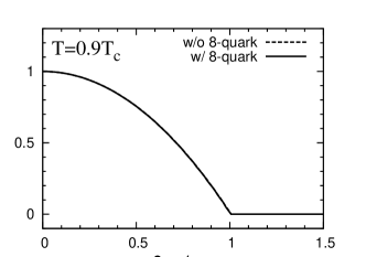
Fig. 3: Effect of scalar-type eight-quark interaction on average phase factor. Solid and dashed lines stand for the PNJL result with and without the eight-quark interaction, respectively.

Figure 4 presents a boundary of the $\langle e^{2i\theta}\rangle=0$ region and locations of CEP calculated by the PNJL model without and with the scalar-type eight-quark interaction. The eight-quark interaction makes the region smaller. Meanwhile, it shifts the CEP to higher $T$ and lower $\mu_{\rm q}$. Thus, the relative distance of CEP to the boundary becomes much smaller by the scalar-type eight-quark interaction, although CEP itself lies in the $\langle e^{2i\theta}\rangle=0$ region even after the scalar-type eight-quark interaction is taken into account. If more accurate LQCD data becomes available in future outside the region $\langle e^{2i\theta}\rangle=0$, the PNJL model that reproduces the data can predict a location of CEP in principle. The reliability of the prediction may be proportional to the relative distance. In this sense, the fact that the relative distance is small is important.

Fig. 4: Effect of the scalar-type 8-quark interaction on locations of CEP and the boundary of the $\langle e^{2i\theta}\rangle=0$ region. Solid and dashed lines stand for the boundary calculated by the PNJL model with and without the eight-quark interaction, respectively. Symbols $+$ and $\times$ mean the CEP calculated by the PNJL model with and without the eight-quark interaction, respectively.

Figure 5 presents contours of $\langle e^{2i\theta}\rangle$ and $\Phi$ in $\mu_{\rm q}$-$T$ plane calculated by the PNJL model with scalar-type eight-quark interaction. Solid curves correspond to contours of $\langle e^{2i\theta}\rangle=0,0.4,$ and 0.8, while dashed curves do to contours of $\Phi=0.3,0.5$ and $0.7$. For $\mu_{\rm q}<m_{\pi}/2$, the average phase factor is finite and then calculable with LQCD in principle. For $\mu_{\rm q}>m_{\pi}/2$, $\langle e^{2i\theta}\rangle=0$ at $\Phi\mathrel{\mathchoice{\lower 3.6pt\vbox{\halign{$\mathsurround=0pt\displaystyle\hfil#\hfil$\cr<\crcr\sim\crcr}}}{\lower 3.6pt\vbox{\halign{$\mathsurround=0pt\textstyle\hfil#\hfil$\cr<\crcr\sim\crcr}}}{\lower 3.6pt\vbox{\halign{$\mathsurround=0pt\scriptstyle\hfil#\hfil$\cr<\crcr\sim\crcr}}}{\lower 3.6pt\vbox{\halign{$\mathsurround=0pt\scriptscriptstyle\hfil#\hfil$\cr<\crcr\sim\crcr}}}}0.5$ corresponding to the confinement region. At $\Phi\mathrel{\mathchoice{\lower 3.6pt\vbox{\halign{$\mathsurround=0pt\displaystyle\hfil#\hfil$\cr>\crcr\sim\crcr}}}{\lower 3.6pt\vbox{\halign{$\mathsurround=0pt\textstyle\hfil#\hfil$\cr>\crcr\sim\crcr}}}{\lower 3.6pt\vbox{\halign{$\mathsurround=0pt\scriptstyle\hfil#\hfil$\cr>\crcr\sim\crcr}}}{\lower 3.6pt\vbox{\halign{$\mathsurround=0pt\scriptscriptstyle\hfil#\hfil$\cr>\crcr\sim\crcr}}}}0.5$ corresponding to the deconfinement region, the factor $\langle e^{2i\theta}\rangle$ is finite and an increasing function of $\Phi$, indicating that there is a positive correlation between $\langle e^{2i\theta}\rangle$ and $\Phi$. Thus, LQCD is feasible only in the deconfinement phase, when $\mu_{\rm q}>m_{\pi}/2$.

Fig. 5: Contours of the average phase factor and the Polyakov loop in $\mu_{\rm q}$-$T$ plane. Contours of $\langle e^{2i\theta}\rangle=0,0.4,0.8$ and 1 are drawn by solid curves, while those of $\Phi=0.3,0.5$ and $0.7$ are by dashed curves.

III.3 Dynamical mesonic fluctuations

The average phase factor was calculated with LQCD Elia and Lombardo (2003) in which the lattice size is $16^{3}\times 4$ and the pion mass at vacuum is $m_{\pi}^{\rm LQCD}\approx 280$ MeV. In the PNJL calculation, we have then varied the quark mass from $m_{0}=5.5$ MeV to $22.5$ MeV to reproduce $m_{\pi}^{\rm LQCD}=280$ MeV. For this value of $m_{0}$, the deconfinement transition temperature becomes a bit higher value, i.e., $T_{\rm c}=180$ MeV.

Fig. 6: Effects of mesonic fluctuations on the average phase factor. All the calculations take account of the eight-quark interaction. In MF+DF and MF+DF2 calculations, $m_{\pi}=m_{\pi}^{\rm LQCD}$ and $2.8m_{\pi}^{\rm LQCD}$, respectively.

Figure 6 shows $\mu_{\rm q}$ dependence of the average phase factor at $T=0.9T_{\rm c},T_{\rm c}$ and $1.25T_{\rm c}$. LQCD result is evaluated from LQCD data at imaginary chemical by assuming a polynomial function. For each panel, the two solid lines delimit the 90% confidence level region for the extrapolation, while the MF+SF calculation is represented by dotted lines. The MF+SF calculation overestimates LQCD data largely. Therefore, we consider dynamical mesonic fluctuations beyond the MF+SF framework.

Below $T_{\rm c}$ where the system is confined, it is natural to think that mesonic modes dominate rather than quark modes. Therefore, we should take all possible channels (mesonic modes) in the bubble summation in the random phase approximation (RPA). If there is no pion condensate, $\sigma$ and $\pi$ meson modes are decoupled to each other. Hence, the mesonic polarization function matrix does not have off-diagonal elements. Up to order $1/N_{\rm c}$, where $N_{\rm c}$ is the number of colors, the thermodynamic potential is obtained by

$$\Omega=\Omega_{\rm MF}+\Omega_{\rm DF},$$ (29)

where $\Omega_{\rm MF}$ is the mean-field part shown in (18) and $\Omega_{\rm DF}$ is the dynamical mesonic fluctuation (DF) part in the ring diagram. Hence, $\Omega_{\rm DF}$ is obtained by Zhuang

$$\Omega_{\rm DF}=-\frac{i}{2}\int\frac{d^{4}q}{(2\pi)^{4}}\ln\det[1-G^{*}_{\rm s}\Pi(q)]$$ (30)

with the effective coupling $G_{\rm s}^{*}={\rm diag}(G^{*}_{{\rm s}j})$ for

$$G^{*}_{{\rm s}\sigma}=\frac{\partial M}{\partial\sigma},~{}~{}~{}G^{*}_{{\rm s}\pi_{+}}=G^{*}_{{\rm s}\pi_{-}}=G^{*}_{{\rm s}\pi_{0}}=\frac{\partial N}{\partial\pi},$$ (31)

and the mesonic polarization bubbles

$$\Pi_{jk}(q) = i\int\frac{d^{4}p}{(2\pi)^{4}}{\rm Tr}[\Gamma^{*}_{j}{\cal S}(p+q)\Gamma_{k}{\cal S}(p)]$$ (32)

for $j,~{}k=\sigma,~{}\pi_{+},~{}\pi_{-},~{}\pi_{0}$, where Tr is the trace in color, flavor and Dirac indexes and the four momentum integral is defined as $\int d^{4}q/(2\pi)^{4}=iT\sum_{n}\int d^{3}{\bf q}/(2\pi)^{3}$ for finite temperature. The meson vertexes $\Gamma_{k}$ depend on meson taken; precisely, $\Gamma_{\sigma}=1,~{}\Gamma_{\pi_{+}}=i\tau_{+}\gamma_{5},~{}\Gamma_{\pi_{-}}=i\tau_{-}\gamma_{5},~{}\Gamma_{\pi_{0}}=i\tau_{3}\gamma_{5}$.

Before calculating dynamical mesonic fluctuations, we clarify a relation between static and dynamical mesonic fluctuations. The effective action of the NJL-type model to $1/N_{\rm c}$ order is derivable by using the auxiliary field method Kashiwa et al (2006). The second derivative of the effective action with respect to meson fields yields the inverse meson propagator $G^{*}_{\rm s}[1-G^{*}_{\rm s}\Pi(q)]$. Since the static fluctuations are constant, the Hessian matrix (27) is obtained by setting the external momentum $q=0$ in the inverse propagator:

$$H=G^{*}_{\rm s}[1-G^{*}_{\rm s}\Pi(q=0)].$$ (33)

Setting $q=0$ in (30) reduces $\Omega_{\rm DF}$ to $\ln\det[H]$ and the resultant partition function turns out to be (24). Thus, the static mesonic fluctuation $\Omega_{\rm SF}=\ln\det[H]$ can be regarded as an approximation to the dynamical one $\Omega_{\rm DF}$.

Now we introduce the effective meson mass $m_{j}^{*}$ which satisfy

$$\det[1-G_{\rm s}^{*}\Pi(q_{0}+\mu_{j}=m_{j}^{*},{\bf q=0})]=0$$ (34)

with the meson chemical potentials $\mu_{\sigma}=\mu_{\pi_{0}}=0$, $\mu_{\pi_{+}}=2\mu_{\rm I}$ and $\mu_{\pi_{-}}=-2\mu_{\rm I}$. Here note that physical meson masses are not $m_{j}^{*}$ but $m_{j}=m_{j}^{*}-\mu_{j}$ because they are calculated from $q_{0}$.

Since it is difficult to calculate the dynamical mesonic fluctuations (30) exactly, here we make the pole approximation that neglects the scattering phase shift. If $T<T_{\rm c}$ and there is no pion condensation, $m_{j}^{*}$ is well approximated by the meson mass $m_{j}^{0}$ at vacuum. In this approximation, $\Omega_{\rm DF}$ can be obtained by a sum of four quasiparticles, $\sigma$, $\pi^{+}$, $\pi^{-}$ and $\pi^{0}$:

$$\Omega_{\rm DF} = \sum_{j}\Omega_{j},$$ (35)

$$\Omega_{j} = \int\frac{d^{3}{\bf q}}{(2\pi)^{3}}\left[\frac{1}{2}(E_{j}-\mu_{j})+T\ln\left(1-e^{-\beta(E_{j}-\mu_{j})}\right)\right],$$

where $E_{j}=\sqrt{{\bf q}^{2}+{m^{*}}^{2}_{j}}$. However, corrections due to $\sigma$ and $\pi^{0}$ mesons are exactly cancelled out between $\Omega_{1+1}$ and $\Omega_{1+1^{*}}$. This framework is referred to as MF+DF in this paper; here, the static fluctuations of $\phi_{3}$ and $\phi_{8}$ are taken into account in the Hessian matrix.

As seen in Fig. 6, at lower $T$ such as $T=0.9T_{\rm c}$ and $T_{\rm c}$, the MF+DF calculation (dashed line) almost reproduces LQCD data. Above $T_{\rm c}$ such as $T=1.25T_{\rm c}$, the MF+DF calculation underestimates LQCD data. For $T>T_{\rm c}$, in general, the pion mass becomes larger than $m^{0}_{\pi}$ Xiong (2009). If $m_{\pi}=2.8m^{0}_{\pi}$ is taken, the calculation (dot-dashed line) is consistent with LQCD data; this calculation is denoted by MF+DF2 in Fig. 6.

IV Summary

We have calculated the average phase factor of the QCD determinant at finite quark chemical potential $\mu_{\rm q}$, using the two-flavor version of the PNJL model with the scalar-type eight quark interaction, since the model is successful in reproducing LQCD data not only on the 1+1 system in the limit of no $\mu_{\rm q}$ Sakai et al (2009) but also on the $1$+$1^{*}$ system with finite isospin chemical potential $\mu_{\rm I}$ Sasaki et al. (2009). In the present model, there exists a critical endpoint (CEP) in the 1+1 system with finite $\mu_{\rm q}$. The CEP lies inside the $\langle e^{2i\theta}\rangle=0$ region. This implies that the location cannot be determined by LQCD solely.

For $\mu_{\rm q}>m_{\pi}/2$, the pion condensate occurs at $\Phi\mathrel{\mathchoice{\lower 3.6pt\vbox{\halign{$\mathsurround=0pt\displaystyle\hfil#\hfil$\cr<\crcr\sim\crcr}}}{\lower 3.6pt\vbox{\halign{$\mathsurround=0pt\textstyle\hfil#\hfil$\cr<\crcr\sim\crcr}}}{\lower 3.6pt\vbox{\halign{$\mathsurround=0pt\scriptstyle\hfil#\hfil$\cr<\crcr\sim\crcr}}}{\lower 3.6pt\vbox{\halign{$\mathsurround=0pt\scriptscriptstyle\hfil#\hfil$\cr<\crcr\sim\crcr}}}}0.5$, so that $\langle e^{2i\theta}\rangle=0$ there. At $\Phi\mathrel{\mathchoice{\lower 3.6pt\vbox{\halign{$\mathsurround=0pt\displaystyle\hfil#\hfil$\cr>\crcr\sim\crcr}}}{\lower 3.6pt\vbox{\halign{$\mathsurround=0pt\textstyle\hfil#\hfil$\cr>\crcr\sim\crcr}}}{\lower 3.6pt\vbox{\halign{$\mathsurround=0pt\scriptstyle\hfil#\hfil$\cr>\crcr\sim\crcr}}}{\lower 3.6pt\vbox{\halign{$\mathsurround=0pt\scriptscriptstyle\hfil#\hfil$\cr>\crcr\sim\crcr}}}}0.5$, the factor $\langle e^{2i\theta}\rangle$ is finite and an increasing function of $\Phi$. Thus, there exists a positive correlation between $\langle e^{2i\theta}\rangle$ and $\Phi$. Therefore, LQCD is feasible only in the deconfinement phase with large $\Phi$, when $\mu_{\rm q}>m_{\pi}/2$.

The eight-quark interaction makes the $\langle e^{2i\theta}\rangle=0$ region shrink, while it shifts the CEP toward higher $T$ and smaller $\mu_{\rm q}$. As a consequence of these properties, a relative distance of the CEP to the boundary of the $\langle e^{2i\theta}\rangle=0$ region becomes smaller. If more accurate LQCD data becomes available in future outside the $\langle e^{2i\theta}\rangle=0$ region, we can predict a location of the CEP with the PNJL model the parameters of which are fitted to the data. The accuracy of the model prediction seems to be proportional to the distance. In this sense, the fact that the relative distance is small is important.

For $\mu_{\rm q}<m_{\pi}/2$ where no pion condensate takes place, the PNJL calculation with static fluctuations cannot reproduce LQCD data Elia and Lombardo (2003) at both $T\leq T_{\rm c}$ and $T>T_{\rm c}$. This problem is solved partly by treating dynamical mesonic fluctuations with the pole approximation. The PNJL model with the dynamical mesonic fluctuations reproduces LQCD data at $T\leq T_{\rm c}$. For $T>T_{\rm c}$, however, the calculation cannot reproduce the data. The first possible reason is that the meson mass at $T>T_{\rm c}$ is different from the value at vacuum. The second possible reason is that the pole approximation is not good, because meson at $T>T_{\rm c}$ is generally in a resonance state. The third possible reason is effects of physical states with nonzero baryon numbers. It is reported in Ref. Elia and Lombardo (2003) that the physical states tend to enhance the average phase factor, although the PNJL model does not include such effects. This problem should be solved in future in order to construct a reliable effective model that makes it possible to predict a location of CEP and the phase diagram at finite $\mu_{\rm q}$.