Lensing reconstruction of cluster-mass cross-correlation with cosmic microwave background polarization

Abstract

We extend our maximum likelihood method for reconstructing the cluster-mass cross-correlation from cosmic microwave background (CMB) temperature anisotropies and develop new estimators that utilize six different quadratic combinations of CMB temperature and polarization fields. Our maximum likelihood estimators are constructed with delensed CMB temperature and polarization fields by using an assumed model of the convergence field and they can be iteratively applied to a set of clusters, approaching to the optimal condition for the lensing reconstruction as the assumed initial model is refined. Using smoothed particle hydrodynamics simulations, we create a catalog of realistic clusters obtainable from the current Sunyaev-Zel’dovich (SZ) surveys, and we demonstrate the ability of the maximum likelihood estimators to reconstruct the cluster-mass cross-correlation from the massive clusters. The iTT temperature estimator provides a signal-to-noise ratio of a factor 3 larger than the iEB polarization estimator, unless the detector noise for measuring polarization anisotropies is controlled under $3\mu{\rm K}$.

I Introduction

In the past few years we have seen rapid development in the measurements of cosmic microwave background (CMB) anisotropies on arcminute scales. Higher precision measurements of CMB temperature anisotropies are available from the completed missions such as the Arcminute Cosmology Bolometer Array Receiver Reichardt et al. (2009) and the Cosmic Background Imager Sievers et al. (2009) and the ongoing experiments with better angular resolution and multi-frequency channels such as the Atacama Cosmology Telescope (ACT, Hincks et al. (2009)) and the South Pole Telescope (SPT, Staniszewski et al. (2008)). While most of the current polarization experiments are aimed at measuring CMB polarization anisotropies on large scales, ACT and SPT will be capable of measuring CMB polarization anisotropies on arcminute scales.

Especially, ACT and SPT are designed for measuring the Sunyaev-Zel’dovich (SZ) effect arising from the Thomson scattering off hot electrons in clusters and thereby detecting massive clusters. These SZ surveys can explore the growth of structure by measuring the abundance of massive clusters and the expansion history of the universe by measuring their correlation functions to probe the evolution of dark energy (see, e.g., Albrecht et al. (2006)). With precisely measured distance and their omnipresence behind all the clusters, CMB anisotropies can be used as a distant background source for weak lensing measurements, providing the cluster-mass cross-correlation and complementing the measurements of cluster mass and their abundance from the same SZ surveys. Moreover, weak lensing measurements of the CMB can be combined with galaxy weak lensing measurements of the same clusters from optical follow-up surveys to measure the source distance ratios in a model-independent way, constraining the expansion history of the universe Hu et al. (2007a).

Weak lensing of the CMB by large-scale structure is efficiently probed by using quadratic estimators, measuring the deviation of the correlation function of CMB anisotropies from the otherwise statistically isotropic correlation Hu (2001). However, it was shown that the standard method of using quadratic estimators is compromised Maturi et al. (2005) on cluster scales and needs additional free parameters Hu et al. (2007b) for calibration, as this method rests on the linear approximation in the lensing effect which breaks down near massive clusters. This problem was tackled by delensing the observed CMB temperature field and analyzing the likelihood of the delensed fields Yoo and Zaldarriaga (2008).

We showed that if the assumed initial model for delensing is a good approximation to the true underlying matter distribution, our new estimator based on the delensed CMB temperature fields becomes an optimal estimator and it can be iteratively applied to given measurements of CMB temperature anisotropies, until the assumed initial model converges to the true matter distribution and the likelihood is maximized. Here we extend our maximum likelihood estimation method for reconstructing the cluster-mass cross-correlation with CMB temperature anisotropies and apply it to CMB polarization anisotropies, yielding new maximum likelihood estimators with six different quadratic combinations of CMB temperature and polarization fields. We demonstrate their applicability by using realistic clusters that can be found in the current CMB experiments.

The rest of the paper is organized as follows. We briefly review the formalism for weak lensing of CMB anisotropies and derive our maximum likelihood estimators in Sec. II. In Sec. III we describe our numerical simulations to model realistic clusters and we construct a catalog of massive clusters with CMB secondary anisotropies. We reconstruct the cluster-mass cross-correlation by using our maximum likelihood estimators and quantify their signal-to-noise ratios in Sec. IV.1, and we investigate the impact of the kSZ contamination in Sec. IV.2. We summarize our findings and conclude in Sec. V. For illustrative purposes, we adopt a flat $\Lambda$CDM universe with cosmological parameters ($\Omega_{m}h^{2}=0.127$, $\Omega_{b}h^{2}=0.0222$, $h=0.73$, $n_{s}=0.95$, $\sigma_{8}=0.78$), consistent with the recent estimation (e.g., (Tegmark and et al., 2006; Komatsu et al., 2008)).

II Formalism

II.1 Weak lensing of CMB polarization

Gravitational lensing is a surface brightness conserving process and it simply redistributes the intrinsic CMB temperature and polarization fields. Here we use $T$, $Q$, and $U$ to represent the CMB temperature and the Stokes parameters for the CMB polarization in units of $\mu{\rm K}$ and use tildes to indicate that the corresponding field is gravitationally lensed. The lensed CMB temperature and polarization fields at the angular position ${\bf\hat{n}}$ on the sky are therefore

$$\tilde{T}({\bf\hat{n}}) = T\left[{\bf\hat{n}}+\hat{\nabla}\phi({\bf\hat{n}})\right]~{},$$ (1)

$$(\tilde{Q}\pm i\tilde{U})({\bf\hat{n}}) = (Q\pm iU)\left[{\bf\hat{n}}+\hat{\nabla}\phi({\bf\hat{n}})\right]~{},$$

and the projected potential

$$\phi({\bf\hat{n}})=-2\int_{0}^{D_{\star}}dD~{}{D_{\star}-D\over DD_{\star}}~{}\psi~{}(D{\bf\hat{n}},D)~{}$$ (2)

describes the deflection angle $\hat{\nabla}\phi({\bf\hat{n}})$ on the sky, where the gravitational potential is $\psi$, the comoving angular diameter distance to the CMB last scattering surface is $D_{\star}=14.12$ Gpc Komatsu et al. (2008), and $\hat{\nabla}$ is the derivative with respect to unit angular vector ${\bf\hat{n}}$. The projected potential $\phi$ is related to the convergence $\kappa$ as $\hat{\nabla}^{2}\phi=-2\kappa$ and it is further related to the physical matter density $\delta\rho_{m}$ projected along the line-of-sight as

$$\kappa({\bf\hat{n}})=\int_{0}^{D_{\star}}dD~{}{D(D_{\star}-D)\over(1+z)^{2}D_{\star}}~{}4\pi G~{}\delta\rho_{m}(D{\bf\hat{n}},D)~{}.$$ (3)

As we are interested in reconstructing the cluster-mass cross-correlation, we adopt the flat sky approximation and express quantities of interest in Fourier space. To linear order in $\phi$, the lensed CMB temperature field can be written as

$$\tilde{T}_{\bf l}=T_{\bf l}-\int{d^{2}{\bf l}_{1}\over(2\pi)^{2}}~{}({\bf l}_{2}\cdot{\bf l}_{1})~{}\phi_{{\bf l}_{2}}~{}T_{{\bf l}_{1}}~{},$$ (4)

with ${\bf l}_{2}={\bf l}-{\bf l}_{1}$ and this equation is also valid for the lensed Stokes parameters $\tilde{Q}_{\bf l}$ and $\tilde{U}_{\bf l}$ in Fourier space. However, since density fluctuations excite only curl-free polarization, the CMB polarization fields are better described by two parity eigenstates, $E$- and $B$-modes Seljak and Zaldarriaga (1997) as $(Q_{\bf l}\pm iU_{\bf l})=(E_{\bf l}\pm iB_{\bf l})e^{\pm 2i\varphi_{\bf l}}$ with the phase $\varphi_{\bf l}$ of the wavevector ${\bf l}$. The lensed CMB polarization fields are therefore

$$\tilde{E}_{\bf l} = E_{\bf l}-\int{d^{2}{\bf l}_{1}\over(2\pi)^{2}}~{}({\bf l}_{2}\cdot{\bf l}_{1})~{}\phi_{{\bf l}_{2}}~{}E_{{\bf l}_{1}}\cos 2\Delta\varphi_{{\bf l}_{1}}~{},$$ (5)

$$\tilde{B}_{\bf l} = -\int{d^{2}{\bf l}_{1}\over(2\pi)^{2}}~{}({\bf l}_{2}\cdot{\bf l}_{1})~{}\phi_{{\bf l}_{2}}~{}E_{{\bf l}_{1}}\sin 2\Delta\varphi_{{\bf l}_{1}}~{},$$

and the lensed CMB power spectra are related to the intrinsic CMB power spectra as

$$\tilde{C}^{T}_{l} = \left[1-l^{2}R\right]C^{T}_{l}+\int{d^{2}{\bf l}_{1}\over(2\pi)^{2}}~{}({\bf l}_{2}\cdot{\bf l}_{1})^{2}~{}C^{\phi}_{l_{2}}~{}C^{T}_{l_{1}}~{},$$ (6)

$$\tilde{C}^{E}_{l} = \left[1-l^{2}R\right]C^{E}_{l}+\int{d^{2}{\bf l}_{1}\over(2\pi)^{2}}~{}({\bf l}_{2}\cdot{\bf l}_{1})^{2}~{}C^{\phi}_{l_{2}}~{}C^{E}_{l_{1}}\cos^{2}2\Delta\varphi_{{\bf l}_{1}},$$

$$\tilde{C}^{C}_{l} = \left[1-l^{2}R\right]C^{C}_{l}+\int{d^{2}{\bf l}_{1}\over(2\pi)^{2}}~{}~{}({\bf l}_{2}\cdot{\bf l}_{1})^{2}~{}C^{\phi}_{l_{2}}~{}C^{C}_{l_{1}}\cos^{2}2\Delta\varphi_{{\bf l}_{1}},$$

$$\tilde{C}^{B}_{l} = \int{d^{2}{\bf l}_{1}\over(2\pi)^{2}}~{}({\bf l}_{2}\cdot{\bf l}_{1})^{2}~{}C^{\phi}_{l_{2}}~{}C^{E}_{l_{1}}\sin^{2}2\Delta\varphi_{{\bf l}_{1}}~{},$$

where $\Delta\varphi_{{\bf l}_{1}}=\varphi_{{\bf l}_{1}}-\varphi_{\bf l}$ and $R=(1/4\pi)\int d\ln l~{}l^{4}C^{\phi}_{l}$ is the half of the rms deflection angle (see, e.g., Hu (2000); Lewis and Challinor (2006)).

Finally, we assume the Gaussian random noise for the detector and the Gaussian beam of the telescope. Therefore, the power spectrum of the detector noise is Knox (1995)

$$C_{l}^{N,T}=\sigma_{\rm pix}^{2}~{}\Omega_{\rm pix}~{},$$ (7)

and the observed CMB temperature field and its power spectrum are

$$\tilde{T}^{\rm obs}_{\bf l} = \tilde{T}_{\bf l}~{}e^{-{1\over 2}l^{2}\sigma_{b}^{2}}+N^{T}_{\bf l}~{},$$ (8)

$$\tilde{C}^{T,{\rm obs}}_{l} = \tilde{C}^{T}_{l}e^{-l^{2}\sigma_{b}^{2}}+C^{N,T}_{l}~{},$$

where $\sigma_{\rm pix}$ is the rms noise of the detector, $\Omega_{\rm pix}$ is the solid angle subtending each pixel of the detector, $N^{T}_{\bf l}$ is the Fourier mode of the detector noise, and the full-width half-maximum (FWHM) of the telescope beam is $\theta_{\rm FWHM}=\sigma_{b}\sqrt{8\ln 2}$ . The observed CMB polarization fields are also described by Eqs. (8), while $\sigma_{\rm pix}$ and $\sigma_{b}$ in CMB polarization experiments may differ from those in CMB experiments for measuring temperature anisotropies.

II.2 Improved quadratic estimators

Matter fluctuations along the line-of-sight deflect CMB photons and this process imprints a deviation of the CMB two-point statistics from statistical isotropy. Quadratic estimators are often used to measure the deviation, but they become progressively biased as the lensing effect increases. This problem can be overcome by using improved quadratic estimators that are constructed by using delensed CMB fields Yoo and Zaldarriaga (2008). Here we briefly review the standard quadratic estimators Hu et al. (2007b) using the CMB polarization fields, on which our improved quadratic estimators are based, and then we describe how our improved quadratic estimators can be used to reconstruct the cluster-mass cross-correlation.

With the CMB temperature and polarization fields, we can construct six convergence estimators $\hat{\kappa}^{XY}({\bf\hat{n}})$ that use two CMB temperature and polarization fields $X,Y=T,E,B$, permitting repetition (hence they are quadratic estimators). The estimators $\hat{\kappa}^{XY}({\bf\hat{n}})$ are symmetric with two fields $X$ and $Y$ interchanged and we use quantities with a hat to indicate that they are estimators thereof (not to be confused with unit angular vectors on the sky). The six convergence estimators are uniquely determined with the requirement that each estimator be unbiased $\langle\hat{\kappa}^{XY}({\bf\hat{n}})\rangle=\kappa({\bf\hat{n}})$  over an ensemble average of the CMB temperature and polarization fields $X$ and $Y$, and the variance of the estimator be minimal Hu (2001),

$$\langle\hat{\kappa}^{XY}_{\bf l}\hat{\kappa}^{*XY}_{{\bf l}^{\prime}}\rangle=(2\pi)^{2}~{}\delta^{D}({\bf l-l^{\prime}})(C^{\kappa}_{l}+N^{\kappa,XY}_{l})~{}.$$ (9)

These estimators can be easily computed in configuration space by using the two Wiener-filtered functions

$${\bf G}_{XY}({\bf\hat{n}})=\int\!\!\!{d^{2}{\bf l}\over(2\pi)^{2}}~{}i{\bf l}\tilde{X}^{\rm obs}_{\bf l}{C_{l}^{XY}\over\tilde{C}^{X,{\rm obs}}_{l}}\bigg{\{}\begin{array}[]{c}e^{2i\varphi_{{\bf l}}}\\ e^{2i\varphi_{{\bf l}}}\end{array}\bigg{\}}e^{-{1\over 2}l^{2}\sigma_{b}^{2}+i{\bf l}\cdot{\bf\hat{n}}}~{},$$ (12)

$$W_{Y}({\bf\hat{n}})=\int\!\!\!{d^{2}{\bf l}\over(2\pi)^{2}}~{}{\tilde{Y}^{\rm obs}_{\bf l}\over\tilde{C}^{Y,{\rm obs}}_{l}}\bigg{\{}\begin{array}[]{c}e^{2i\varphi_{{\bf l}}}\\ ie^{2i\varphi_{{\bf l}}}\end{array}\bigg{\}}e^{-{1\over 2}l^{2}\sigma_{b}^{2}+i{\bf l}\cdot{\bf\hat{n}}}~{},$$ (15)

with the phase angle $\varphi_{\bf l}$ of the wavevector ${\bf l}$ and two phase factors for $Y=E,B$ in the braces. Note that $C_{l}^{XY}=C_{l}^{XE}$ for $Y=B$ and the phase factor in the braces is unity for $Y=T$. The convergence estimator is then

$$\hat{\kappa}^{XY}_{\bf l}=-{N^{XY}_{l}\over 2}~{}i{\bf l}\cdot\int d^{2}{\bf\hat{n}}~{}{\rm Re}\left[{\bf G}_{XY}({\bf\hat{n}})W_{Y}^{*}({\bf\hat{n}})\right]~{}e^{-i{\bf l}\cdot{\bf\hat{n}}}~{}.$$ (16)

The normalization coefficients $N^{XY}_{l}$ are related to the noise power spectrum $N^{\kappa,XY}_{l}$ of XY estimators $\hat{\kappa}^{XY}({\bf\hat{n}})$ as $N^{\kappa,XY}_{l}=l^{2}N^{XY}_{l}/4$, and they can be obtained as

$${1\over N^{XY}_{l}} = {1\over l^{2}}\int{d^{2}{\bf l}_{1}\over(2\pi)^{2}}{({\bf l}\cdot{\bf l}_{1})~{}C^{XY}_{l_{1}}f^{XY}_{{\bf l}_{1}{\bf l}_{2}}\over\tilde{C}^{X,{\rm obs}}_{l_{1}}~{}\tilde{C}^{Y,{\rm obs}}_{l_{2}}}$$ (17)

$$\times \bigg{\{}\begin{array}[]{c}\cos 2\Delta\varphi\\ \sin 2\Delta\varphi\end{array}\bigg{\}}~{}e^{-l_{1}^{2}\sigma_{b}^{2}}~{}e^{-l_{2}^{2}\sigma_{b}^{2}}~{},$$ (20)

with ${\bf l}={\bf l}_{1}+{\bf l}_{2}$, $\Delta\varphi=\varphi_{{\bf l}_{1}}-\varphi_{{\bf l}_{2}}$, and $\langle X_{{\bf l}_{1}}Y_{{\bf l}_{2}}\rangle=f_{{\bf l}_{1}{\bf l}_{2}}^{XY}~{}\phi_{\bf l}$ , where

$$f^{TT}_{{\bf l}_{1},{\bf l}_{2}} = ({\bf l}\cdot{\bf l}_{1})~{}C^{T}_{l_{1}}+({\bf l}\cdot{\bf l}_{2})~{}C^{T}_{l_{2}}~{},$$ (21)

$$f^{TE}_{{\bf l}_{1},{\bf l}_{2}} = ({\bf l}\cdot{\bf l}_{1})~{}C^{C}_{l_{1}}\cos 2\Delta\varphi+({\bf l}\cdot{\bf l}_{2})~{}C^{C}_{l_{2}}~{},$$

$$f^{TB}_{{\bf l}_{1},{\bf l}_{2}} = ({\bf l}\cdot{\bf l}_{1})~{}C^{C}_{l_{1}}\sin 2\Delta\varphi~{},$$

$$f^{EE}_{{\bf l}_{1},{\bf l}_{2}} = \left[({\bf l}\cdot{\bf l}_{1})~{}C^{E}_{l_{1}}+({\bf l}\cdot{\bf l}_{2})~{}C^{E}_{l_{2}}\right]\cos 2\Delta\varphi~{},$$

$$f^{EB}_{{\bf l}_{1},{\bf l}_{2}} = ({\bf l}\cdot{\bf l}_{1})~{}C^{E}_{l_{1}}\sin 2\Delta\varphi~{}$$

(see Hu and Okamoto (2002); Hu et al. (2007b) for details). Due to the vanishing signal-to-noise ratio, no quadratic BB estimator is used.

Improved quadratic estimators are similar in many aspects to the above standard quadratic estimators. Our estimation process is as follows: Improved quadratic estimators take an initial model $\kappa^{m}({\bf\hat{n}})$ of the convergence field and we first compute the delensed CMB temperature and polarization fields $X^{d}({\bf\hat{s}})=\tilde{X}^{\rm obs}({\bf\hat{n}})$ by solving the lensing equation ${\bf\hat{s}}={\bf\hat{n}}+\hat{\nabla}\phi^{m}({\bf\hat{n}})$, where the initial model $\phi^{m}({\bf\hat{n}})$ for the projected potential is related to $\kappa^{m}({\bf\hat{n}})$ as $\hat{\nabla}^{2}\phi^{m}({\bf\hat{n}})=-2~{}\kappa^{m}({\bf\hat{n}})$ . Improved quadratic estimators are constructed by using the same Wiener-filtered functions ${\bf G}_{XY}({\bf\hat{n}})$ and $W_{Y}({\bf\hat{n}})$ but with the delensed CMB temperature and polarization fields $X^{d}$ and $Y^{d}$ rather than $\tilde{X}^{\rm obs}$ and $\tilde{Y}^{\rm obs}$ themselves, and Eq. (16) yields the change $\Delta\kappa^{XY}({\bf\hat{n}})$ in the convergence field with respect to the assumed initial model $\kappa^{m}({\bf\hat{n}})$. The resulting convergence field $\kappa^{m}({\bf\hat{n}})+\Delta\kappa^{XY}({\bf\hat{n}})$ then serves as a refined initial model for the next iteration and this process is iterated until the numerical convergence is achieved $\Delta\kappa^{XY}({\bf\hat{n}})/\kappa^{m}({\bf\hat{n}})\ll 1$. In practice, one can try different initial models for a faster numerical convergence, when $\Delta\kappa^{XY}({\bf\hat{n}})\simeq\kappa^{m}({\bf\hat{n}})$.

While our improved quadratic estimators take the same functional form as the standard quadratic estimators (thereby its name is inherited), there exist critical differences: Our improved quadratic estimators are based on the maximum likelihood of the delensed CMB temperature and polarization fields, and the iteration process is indeed the standard Newton-Raphson method for maximizing the likelihood of each estimate given the observed CMB temperature and polarization fields. Since the initial model $\kappa^{m}({\bf\hat{n}})$ that depends on the previous iteration process is refined and the refined model $\kappa^{m}+\Delta\kappa$ becomes a new initial model in the following iteration, the improved quadratic estimators are in fact rational functions of the CMB temperature and polarization fields, rather than quadratic functions, making full use of the information contained in the likelihood.

Furthermore, our improved quadratic estimators are free from the approximation that the lensing effect is weak, the breakdown of which plagues the standard quadratic estimators. Consequently, there is no arbitrary cutoff scale used in modified quadratic estimators Hu et al. (2007b) that breaks the symmetry in the convergence estimators when the CMB temperature and polarization fields $X$ and $Y$ are interchanged. Hereafter, we refer to improved quadratic estimators using delensed CMB temperature and polarization fields $X$ and $Y$ as iXY estimators.

III Massive Clusters

We describe our model for massive clusters in Sec. III.1 and discuss possible contaminants for lensing reconstruction arising from secondary anisotropies in the CMB temperature and polarization fields in Sec. III.2. Tests of the applicability of our improved quadratic estimators to realistic clusters are presented in Sec. IV.

III.1 Numerical simulation

Here we model massive clusters using the numerical simulations of Springel and Hernquist (2003). We use the largest volume simulation (G-series) among a number of simulation runs with varying mass and spatial resolution. The smoothed particle hydrodynamics (SPH) simulations were performed using the parallel GADGET code Springel et al. (2001), employing the variational formulation of Springel and Hernquist (2002). We focus on the simulation with $2\times 324^{3}$ of gas and dark matter particles in a comoving cubic volume $(100{h^{-1}{\rm Mpc}})^{3}$. Dark matter halos are identified by applying the friends-of-friends (FoF) group finding algorithm Davis et al. (1985) to the dark matter distribution with a comoving linking length of 0.2 times the mean interparticle separation $62{h^{-1}{\rm kpc}}$. Although the simulation was run in a flat $\Lambda$CDM universe with slightly different cosmological parameters ($\Omega_{m}=0.3$, $\Omega_{\Lambda}=0.7$, $\Omega_{b}=0.04$, $n_{s}=1$, $\sigma_{8}=0.9$), we simply retain the physical properties of the simulation such as particle mass, position, and velocity.

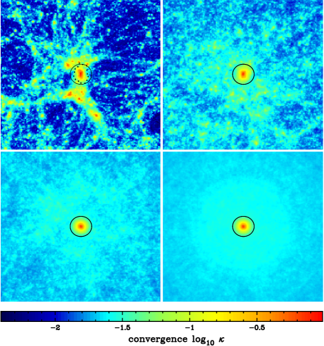
Figure 1: (color online) Average convergence fields $\kappa({\bf\hat{n}})$ of a $40^{\prime}\times 40^{\prime}$ region around massive clusters at $z=1$. Each panel shows $\kappa({\bf\hat{n}})$ obtained by averaging 1 (top left), 10 (top right), 100 (bottom left), and 1000 (bottom right) identical but randomly rotated regions around the massive cluster from the smoothed particle hydrodynamics simulation, which represents different clusters of the same mass. The cluster has of mass $M=3.7\times 10^{14}{h^{-1}M_{\odot}}$ and virial radius $R_{\rm vir}=1.9{h^{-1}{\rm Mpc}}$. Circles show $R_{\rm vir}$ on the sky subtended by 2$.\!^{\prime}$7 and the dotted line in the upper left panel shows the boundary of the cluster members identified by the friends-of-friends algorithm. Once many lines-of-sight are stacked, the average convergence field restores the spherical symmetry.

Figure 2: Convergence profiles $\kappa(\theta)$ around massive clusters at $z=1$. Profiles are obtained by averaging the stacked convergence fields $\kappa({\bf\hat{n}})$ in Fig. 1 over the annulus $\theta$ around the cluster center. Thin and thick lines show the convergence profiles obtained by counting only the cluster members identified by the friends-of-friends algorithm and by counting all the particles within the annulus, respectively. The thick solid line represents the cluster-mass cross-correlation and it deviates substantially from the average cluster mass profile (thin solid) around the virial radius. The average cluster mass profile is well approximated by a projected NFW profile truncated at the virial radius (vertical dotted). Note that dot-dashed lines are largely obscured by solid lines, indicating fast convergence of $\kappa(\theta)$.

To generate a catalog of massive clusters that can be found in the current Sunyaev-Zel’dovich surveys, we first select the most massive halo in the simulation output at $z=1$; The massive halo contains $\sim$150,000 dark matter particles, corresponding to virial mass $M=3.7\times 10^{14}{h^{-1}M_{\odot}}$ and radius $R_{\rm vir}=1.9{h^{-1}{\rm Mpc}}$. Every particle in the simulation is then shifted to have the massive halo at the center of the simulation box by using the periodic boundary condition, and the whole simulation box is randomly rotated to provide the distant observer with different lines-of-sight to the massive cluster. We treat the massive cluster seen at different lines-of-sight as independent clusters of the same mass at $z=1$. This process is necessary to generate a large number of massive clusters using SPH simulations. Since individual clusters identified by the FoF algorithm lack spatial symmetry, snapshots of the cluster at different lines-of-sight are relatively independent of each other as far as the projected matter density is concerned.

Figure 1 shows the convergence fields $\kappa({\bf\hat{n}})$ of a $40^{\prime}\times 40^{\prime}$ region on the sky around the massive cluster with the virial radius indicated as the circle at the center. With the fixed distance $D_{\star}$ to the background source, the critical (physical) surface density is just a function of the redshift of the lensing cluster $1/\Sigma_{\rm crit}=4\pi GD(D_{\star}-D)/D_{\star}(1+z)$ and the convergence is the ratio of the projected mass density $\Sigma({\bf\hat{n}})$ to the critical surface density $\kappa({\bf\hat{n}})=\Sigma({\bf\hat{n}})/\Sigma_{\rm crit}$ . The comoving angular diameter distance to the redshift slice $z=1$ is $D=2400{h^{-1}{\rm Mpc}}$ and the corresponding critical surface density is $\Sigma_{\rm crit}=1800~{}hM_{\odot}{\rm pc}^{-2}$. Here we keep fixed the detector scale $0.\!^{\prime}2$ per pixel, smaller than the typical telescope beam size. Each dark matter particle in the simulation is of mass $m_{\rm dm}=2.1\times 10^{9}{h^{-1}M_{\odot}}$ and it contributes $\kappa=6.0\times 10^{-5}$ per pixel² at $z=1$. Many lines-of-sight are randomly generated and each panel shows $\kappa({\bf\hat{n}})$ averaged over 1, 10, 100, and 1000 different lines-of-sight to the massive cluster, mimicking the process of stacking many different clusters at $z=1$. Once many clusters are stacked, the average convergence field (bottom right) restores the spherical symmetry.

Figure 2 shows the convergence profiles $\kappa(\theta)$ averaged over annulus as a function of angular separation $\theta$ from the cluster center. Each line represents $\kappa(\theta)$ from the average convergence fields obtained by stacking as many clusters indicated in the legend. Projected NFW profiles with truncation at $R_{\rm vir}$ provide a good approximation to the average cluster mass profile (thin solid) obtained by counting only the cluster members identified by the FoF algorithm. However, weak lensing measures the projected mass distribution including contributions from interlopers that happen to lie between the lensing cluster and the observer. The average convergence profile from the stacked field, therefore, provides the cluster-mass cross-correlation (thick solid).

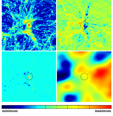
Figure 3: (color online) Kinetic Sunyaev-Zel’dovich (kSZ) effect. Top left: Thomson scattering optical depth $\tau$ of the same region in Fig. 1. We assume the helium mass fraction is $Y_{\rm He}=0.24$ and helium atoms are doubly ionized. Top right: Line-of-sight velocity field $v_{\rm los}$ of dark matter particles. Bottom left: The kSZ effect $\Delta T_{\rm kSZ}/T=-\tau~{}v_{\rm los}/c$. Electrons are assumed to follow the dark matter distribution. Bottom right: $\Delta T_{\rm kSZ}$ from the kSZ effect is superimposed to the intrinsic CMB temperature field. The horizontal color bar represents the scales of each panel in the range of $-4.4\leq\log\tau\leq-2.0$, $-700~{}{\rm km\,s}^{-1}\leq v_{\rm los}\leq 560~{}{\rm km\,s}^{-1}$, $-16~{}\mu{\rm K}\leq\Delta T_{\rm kSZ}\leq 30~{}\mu{\rm K}$, and $-148~{}\mu{\rm K}\leq\Delta T\leq 110~{}\mu{\rm K}$, respectively.

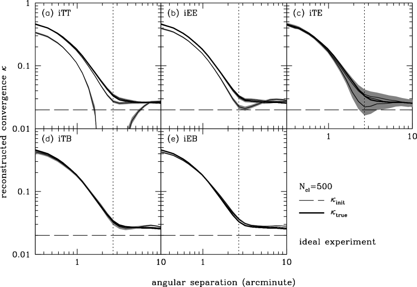
Figure 4: Lensing reconstruction of the convergence profile $\kappa(\theta)$ using improved quadratic estimators based on CMB temperature and polarization fields in an ideal CMB experiment ($\sigma_{\rm pix}=\theta_{\rm FWHM}=0$). The initial model for the convergence field is assumed to have a uniform matter distribution $\kappa^{m}(\theta)=0.02$ (dashed) and improved quadratic estimators are applied to 500 clusters, yielding an estimate of the convergence profile (thin solid) with its uncertainty (shaded) at each iteration, and refining the initial input model. All the improved quadratic estimators converge quickly to the true convergence profile (thick solid) in a few iterations.

III.2 Secondary anisotropies by clusters

On cluster scales, the CMB temperature and polarization fields can be approximated as large-scale gradient fields, and their gradient directions are nearly uncorrelated. Gravitational lensing by massive clusters induce dipolelike wiggles around the clusters to the CMB temperature and polarization gradient fields, and these features are used to measure the lensing effect Seljak and Zaldarriaga (2000). However, there exist several sources of contamination that mimic the lensing signature and complicate its reconstruction process.

Hot electrons in massive clusters scatter off CMB photons, giving rise to a spectral distortion of the otherwise Planck distribution of the CMB temperature field. This thermal Sunyaev-Zel’dovich (tSZ) effect Sunyaev and Zeldovich (1970) can be as large as $\Delta T\simeq 500\mu{\rm K}$ and it is a major source of contamination, significantly exceeding the lensing signals from the clusters. However, with its distinctive spectral signature the tSZ effect can be removed by multi-frequency observations and here we ignore the possible contamination of the residual tSZ effect arising from an imperfect cleaning process. However, the scattering of hot electrons in massive clusters also gives rise to the Doppler effect due to the bulk motion of the clusters. Though smaller than the tSZ effect, this kinetic Sunyaev-Zel’dovich (kSZ) effect Sunyaev and Zeldovich (1972) is comparable to the lensing signals $\Delta T_{\rm kSZ}\simeq 30\mu{\rm K}$ and its identical spectral dependence makes it hard to separate from the intrinsic CMB temperature anisotropies or the lensing signature by clusters.

In contrast to CMB temperature anisotropies, CMB polarization anisotropies have relatively little contamination from the tSZ and kSZ effects; There are a couple of contamination sources in CMB polarization anisotropies such as the scattering of the kinetic quadrupole in the electron’s rest frame, the scattering of the anisotropic CMB photons from the tSZ effect, and double scattering within the cluster (e.g., Sunyaev and Zeldovich (1980); Lewis and King (2006)). However, compared to the lensing effect $\sim 1\mu{\rm K}$ in polarization, the effects of these contaminants are negligible $\ll 0.1\mu{\rm K}$ as they are proportional to $\beta^{2}\tau$, $y\tau$, and $\beta\tau^{2}$ with the tangential velocity $\beta=v_{t}/c\sim 10^{-3}$ and $y=\tau kT_{e}/m_{e}c^{2}\sim 10^{-5}$ (e.g., Amblard and White (2005); Shimon et al. (2006)). Therefore, we only consider the kSZ effect as a contaminant in CMB temperature anisotropies and no contaminant is assumed in CMB polarization anisotropies in the remainder of the paper.

Figure 3 illustrates the kSZ effect around the massive cluster at $z=1$ in Fig. 1. The top panels show the Thomson scattering optical depth $\tau$ and the line-of-sight velocity field $v_{\rm los}$ of free electrons. We assume that the helium mass fraction is $Y_{\rm He}=0.24$ and that gas is fully ionized throughout the simulation box. While the gas distribution in massive clusters may have a velocity dispersion lower than the dark matter distribution, here we simply assume that the gas distribution traces the dark matter distribution in phase space with the universal mass fraction $\Omega_{b}/\Omega_{\rm dm}$ and investigate its impact in Sec. IV.2. Therefore, the top left panel appears identical to the convergence field (top left) in Fig. 1, as they are both proportional to the projected mass density. The cluster is moving toward the observer at the mean $v_{\rm los}=-300~{}{\rm km\,s}^{-1}$ and its $v_{\rm los}$ distribution is random with the rms $\sigma_{v}=640~{}{\rm km\,s}^{-1}$, though the average $v_{\rm los}$ seen in Fig. 3 is smaller due to the inclusion of random interlopers along the line-of-sight within the finite angular size of detector pixel.

The bottom panels show the kSZ effect $\Delta T_{\rm kSZ}/T=-\tau~{}v_{\rm los}/c$ with and without the intrinsic CMB temperature field. Most of the intergalactic medium is transparent ($\tau\simeq 0$) and there is little kSZ effect therein, except a few small blobs along the large-scale filaments. The kSZ effect $\Delta T_{\rm kSZ}\simeq 30\mu{\rm K}$ is highly concentrated at the cluster center and diminishes fast as the matter density of clusters falls off rapidly. However, the contamination from the kSZ effect is apparent in the bottom right panel and its impact increases with redshift as clusters at high redshift are more compact and the line-of-sight velocity decreases only with $(1+z)^{-1/2}$.

IV Reconstructing Cluster-Mass Cross-Correlation

Using the numerical simulation in Sec. III, we demonstrate the applicability of our improved quadratic estimators to realistic clusters. In Sec. IV.1 we first test five improved quadratic estimators in an ideal CMB experiment, and we then compare their performance in realistic CMB experiments. In Sec. IV.2 we discuss the impact of the kSZ contamination on the lensing reconstruction by using CMB temperature anisotropies and comment on a way to improve the reconstruction in the presence of the kSZ effect.

IV.1 Improved quadratic estimators using CMB polarization anisotropies

Here we test our improved quadratic estimators against the numerical simulation described in Sec. III. Figure 4 shows the convergence profiles reconstructed by applying improved quadratic estimators (labeled in the legend of each panel) to 500 clusters at $z=1$ in an ideal experiment with no detector noise ($\sigma_{\rm pix}=0$) and telescope beam ($\theta_{\rm FWHM}=0$). Note that each cluster we stack has different shapes. We first apply improved quadratic estimators by adopting an initial convergence model $\kappa^{m}(\theta)=0.02$ (horizontal dashed), i.e., no lensing signature in the observed CMB temperature and polarization anisotropies. Each estimator takes the assumed initial model and computes the change $\Delta\kappa$ from the assumed model, yielding an estimate (thin solid) of the convergence profile. The first estimates of each of the estimators from the uniform matter distribution are already close to the true convergence profile (thick solid). Having adopted the initial model without lensing effects, our improved quadratic estimators operate as standard quadratic estimators, and they are biased low when the lensing effect is large near the massive clusters Maturi et al. (2005); Hu et al. (2007b); Yoo and Zaldarriaga (2008), while the nonlinear effect is relatively mitigated for iTE, iTB, and iEB estimators, since the lensing contribution is partially canceled due to the oscillating nature of the cross power spectrum $C^{C}_{l}$ and there is no B-mode polarization anisotropy $C^{B}_{l}=0$.

Next we take the estimate (thin line) of the convergence profile in the first trial as our initial convergence model for the next iteration, and we repeat the iteration process until the estimates converge. In just a few iterations, the initial convergence model of the uniform matter distribution is quickly reshaped and all the estimators in each panel converge to the true convergence profile without any detectable bias beyond the cluster virial radius (vertical dotted). The uncertainties (shaded region) in the mean estimate become smaller as the assumed convergence model is refined at each iteration; their minimum is achieved when the estimates converge to the true convergence profile and it is set by the intrinsic fluctuations of CMB temperature and polarization anisotropies. For a faster convergence, one can start with a more realistic initial model of the convergence field motivated by other observations rather than the uniform matter distribution assumed here. Note that while we characterize our reconstruction for the cluster-mass cross-correlation in terms of the convergence profile $\hat{\kappa}(\theta)$ averaged over the annulus, it is the 2D convergence field $\hat{\kappa}({\bf\hat{n}})$ that we reconstruct using improved quadratic estimators (similarly for the initial models).

Figure 5: Relative performance comparison of the improved quadratic estimators for reconstructing the convergence profile. The left panel shows the statistical uncertainties in the mean convergence profile obtained by applying each estimator to 1000 clusters in the fiducial CMB experiment with $\sigma_{\rm pix}=3\mu{\rm K}$ and $\theta_{\rm FWHM}=0.\!^{\prime}5$. The right panel shows the degradation in the total signal-to-noise ratio of each estimator as a function of the detector noise, compared to that of the iTT estimator in the fiducial experiment.

Figure 5 compares the relative performance of each improved quadratic estimator in reconstructing the convergence profile in the fiducial CMB experiment with $\sigma_{\rm pix}=3\mu{\rm K}$ and $\theta_{\rm FWHM}=0.\!^{\prime}5$ and quantifies its signal-to-noise ratio for different CMB experiments with varying levels of detector noise. The left panel plots the statistical uncertainty in the mean estimate of the convergence profile for each estimator from 1000 clusters, after a few iterations when the estimates have converged. The statistical uncertainties are averaged over the logarithmic radial bin, comparing the relative performance and they decrease in proportion to $N_{\rm cl}^{1/2}$ with $N_{\rm cl}$ being the number of clusters stacked.

The performance difference of each estimator in Fig. 5a originates from their noise power spectrum in Eq. (9) and the noise power spectrum $N^{\kappa,XY}_{l}$ of each estimator, or equivalently the normalization $N_{l}^{XY}$ in Eq. (17), is determined by the intrinsic CMB power spectra $C_{l}^{XY}$, $C_{l}^{X}$, and $C_{l}^{Y}$, given experimental specifications (detector noise and telescope beam size). Especially, the relevant information about the lensing reconstruction is contained around $l\sim 1/\theta_{\rm cl}\sim 3000$. Since the intrinsic CMB power spectra decay exponentially, the noise power spectrum $N_{l}^{\kappa,TT}$ for iTT estimators at $l\gg 1/\theta_{\rm cl}$ is set by the sum of the ratios $C^{T}_{l}/C^{N,T}_{l}$ at $l\lesssim l_{\rm crit}$ and $l_{\rm crit}$ is the scale at which the ratio becomes unity ($1/\theta_{\rm cl}<l_{\rm crit}^{TT}$). Analogously, the relevant ratios can be obtained by using Eq. (17) as $C^{E}_{l}/C^{N,E}_{l}$ for iEB and iEE estimators and $(C^{C}_{l})^{2}/C^{N,T}_{l}C^{N,E}_{l}$ for iTB and TE estimators, though the critical scale $l_{\rm crit}$ is similar to the cluster scale, $1/\theta_{\rm cl}\simeq l_{\rm crit}$ for the polarization estimators. Since there is no intrinsic B-mode polarization anisotropy, the noise power spectra of iEB and iTB estimators are somewhat smaller than those of iEE and iTE estimators on cluster scales. Therefore, the lensing reconstruction of the cluster convergence profile can be best achieved by iTT estimators, and iEB, iEE, iTB, and iTE estimators have larger variance in the sequential order for the fiducial CMB experiment as shown in Fig. 5a.

To quantify the signal-to-noise ratio of the improved quadratic estimators and their dependence on the detector noise, we compute the covariance matrix of each estimator as

$$\mathcal{C}_{XY}(\theta,\theta^{\prime})=\left\langle\left[\hat{\kappa}^{XY}(\theta)-\kappa(\theta)\right]\left[\hat{\kappa}^{XY}(\theta^{\prime})-\kappa(\theta^{\prime})\right]\right\rangle~{},$$ (22)

and the signal-to-noise ratio for each experiment specifications is then

$$\Delta\chi^{2}_{XY}=\sum_{\theta,\theta^{\prime}}\kappa(\theta)\left[\mathcal{C}_{XY}(\theta,\theta^{\prime})\right]^{-1}\kappa(\theta^{\prime})~{}.$$ (23)

Since the lensing effect on CMB power spectra is to convolve them with its potential power spectrum $C^{\phi}_{l}$, the lensing estimators are intrinsically non-local and the covariance matrix is non-diagonal Yoo and Zaldarriaga (2008). The covariance matrix is computed by averaging over 50,000 clusters to guarantee its numerical convergence.

Figure 5b plots the ratio of $\Delta\chi^{2}_{TT}$ of the TT estimator in the fiducial experiment to $\Delta\chi_{XY}^{2}$ of each estimator as a function of detector noise. As in Fig. 5a, the general trend of the performance of each estimator remains unchanged over a wide range of detector noise; as the detector noise increases, the performance of all the estimators is progressively degraded. However, the signal-to-noise ratios dramatically improve at $\sigma_{\rm pix}<3\mu{\rm K}$ for the estimators using CMB polarization anisotropies, since at the cluster scale the intrinsic CMB polarization anisotropies are small and easily dominated by the detector noise.

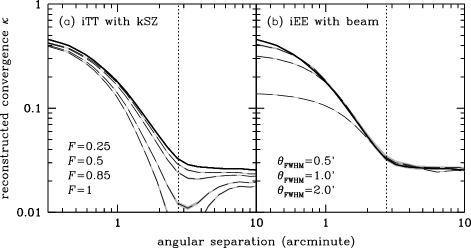
Figure 6: Impact of the kinetic Sunyaev-Zel’dovich (kSZ) effect on the lensing reconstruction. For the fiducial experiment with $\theta_{\rm FWHM}=0.\!^{\prime}5$ and $\sigma_{\rm pix}=3~{}\mu{\rm K}$, we use the simulation in Sec. III to generate 10,000 massive clusters at $z=1$ and stack the convergence profiles reconstructed by applying iTT and iEE estimators. Left panel: Assuming that the gas distribution traces the dark matter distribution in phase space from the simulation, we compute the kSZ contamination as a function of the ionized gas fraction $F$ in Eq. (24). The reconstructed convergence profile is progressively biased in the presence of the kSZ contamination in CMB temperature anisotropies. Right panel: Convergence profiles with iEE estimators as a function of telescope beam. No contamination from the clusters is assumed in CMB polarization anisotropies. Reconstructed convergence profiles are shown as dashed lines with their uncertainty (shaded), while the true convergence profile is shown as solid lines.

IV.2 Kinetic Sunyaev-Zel’dovich effect

Now we use the simulation in Sec. III.2 with its velocity distribution to investigate the effect of the kSZ contamination illustrated in Fig. 3 on the lensing reconstruction. Note that we consider only the kSZ effect as a possible contamination of CMB temperature anisotropies and no other contamination is assumed for CMB polarization anisotropies, except the lensing effect itself (see, Sec. III.2 for estimates of possible contamination in CMB polarization anisotropies).

In massive clusters, baryons make up a universal mass fraction $\Omega_{b}/\Omega_{m}=0.138$ and they exist predominantly in the form of ionized gas in the intracluster medium. However, stars and galaxies in massive clusters contain a non-negligible fraction of baryons, and X-ray observations show that the gas mass fraction is $f_{\rm gas}=0.117$ within $r_{2500}$, which corresponds to $\sim 0.1R_{\rm vir}$: Approximately 85% of the baryons in massive clusters contributes to the kSZ effect (see, e.g., Allen et al. (2002); Vikhlinin et al. (2006) for estimating the gas mass fraction). Here we simply adopt the ionized gas fraction $F$ as a free parameter and the free electron number density is then obtained from the simulation by

$$n_{e}=F\times\left({\Omega_{b}\over\Omega_{\rm dm}}\right)\left[{m_{\rm dm}\over m_{p}}\left(1-{Y_{\rm He}\over 2}\right)\right]~{},$$ (24)

where $m_{p}$ is the proton mass. Since the kSZ effect is proportional to the product of the free electron number density and the line-of-sight velocity, a lower value of $F$ can represent a lower velocity distribution of baryons in massive clusters with the universal mass fraction $\Omega_{b}/\Omega_{m}$.

Figure 6a shows the impact of the kSZ contamination on the lensing reconstruction (dashed) from iTT estimators in the fiducial experiment. When most baryons are contained in the ionized gas ($F=1$ and $F=0.85$), the kSZ contamination is $\Delta T_{\rm kSZ}\simeq 30\mu{\rm K}$ and $25\mu{\rm K}$ at the cluster center, respectively, and its effect is substantially larger than the typical change $\Delta T\simeq 10\mu{\rm K}$ arising from the lensing effect by clusters. Consequently, the lensing reconstruction is significantly biased in the presence of the kSZ contamination. For the other two cases, in which large fraction of the baryons are in stars ($F=0.5$ and $F=0.25$), the kSZ contamination $\Delta T_{\rm kSZ}=15\mu{\rm K}$ and $7.5\mu{\rm K}$ is smaller and its impact is reduced, though the bias in the lensing reconstruction prevails over a range of separations.

Compared to CMB temperature anisotropies, CMB polarization anisotropies are relatively free from secondary contamination and the lensing effect is the dominant source of secondary anisotropies. However, the current CMB experiments such as SPT and ACT lack the ability to measure polarization anisotropies, and other upcoming CMB experiments may not be optimized for measuring the cluster lensing signature in polarization anisotropies. Figure 6b illustrates the lensing reconstruction by using iEE estimators in future CMB polarization experiments with larger telescope beam size (B-mode polarization measurements are even harder due to the vanishing signal). No significant bias develops for iEE estimators within the virial radius. However, as the angular resolution decreases, small scale structure is smoothed and the reconstructed convergence profile is the true convergence profile convolved with the telescope beam (dashed line).

Finally, with the current CMB experiments capable of measuring only temperature anisotropies on cluster scales, we consider a way to mitigate the impact of the kSZ contamination in the lensing reconstruction using CMB temperature anisotropies. Since the kSZ effect arises from the Thomson scattering off free electrons in clusters, its contamination is centrally concentrated as seen in Fig. 3, scaling in proportion to $\kappa(\theta)$. The lensing effect, however, extends well beyond the innermost region of clusters; for example, the kSZ effect falls off as $1/\theta$ in singular isothermal clusters, while the lensing effect remains constant throughout the cluster region. Therefore, the simplest way to reduce the kSZ contamination is to suppress or purge the central region of clusters, where the kSZ effect is strongest (see, e.g., Vale et al. (2004)). Since the lensing estimators are non-local and the information on the central region is shared by lensed CMB temperature anisotropies over the cluster virial radius Yoo and Zaldarriaga (2008), the lensing reconstruction is possible even with the pixels at the innermost region of clusters masked out. However, with our quadratic estimators built in Fourier space, translational invariance prevents from discriminating the central region. We leave the further investigation of how masking the central region affects the performance of our estimator for future work.

V Discussion

We have generalized the maximum likelihood estimators Yoo and Zaldarriaga (2008) for reconstructing the cluster-mass cross-correlation to utilize delensed CMB polarization fields, and we have tested our new maximum likelihood estimators for the lensing reconstruction against numerical simulations. The observed CMB temperature and polarization fields are delensed based on an initial model of the convergence field and our maximum likelihood estimators (called improved quadratic estimators) provide improvements over the assumed initial model. This process can be iterated until numerical convergence is achieved. Compared to the standard and modified quadratic estimators Maturi et al. (2005); Hu et al. (2007b), our improved quadratic estimators have no free parameters and provide unbiased reconstructions even in the regime where the linear approximation in the lensing effect breaks down.

We have adopted smoothed hydrodynamic simulations to model realistic clusters, and the improved quadratic estimators that use six different combinations of CMB temperature and polarization fields can reconstruct the underlying matter distribution in a non-parametric way to obtain the cluster-mass cross-correlation. Their ability to reconstruct the cluster-mass cross-correlation is determined by the ratio of the intrinsic CMB power spectrum to the detector noise power spectrum on cluster scales. Given the same experimental specifications for measuring CMB temperature and polarization anisotropies, iTT estimators can reconstruct the cluster-mass cross-correlation by a factor of 3 in the signal-to-noise ratio, better than iEB estimators, which are better suited for reconstructing large-scale structure.

For the gas mass fraction $f_{\rm gas}=0.117$, the numerical simulations show that the kinetic Sunyaev-Zel’dovich (kSZ) contamination is $\Delta T_{\rm kSZ}\simeq 30\mu{\rm K}$ at the innermost region of clusters. As clusters are more compact at high redshift with weak redshift dependence of their peculiar velocity, the spectrally indistinguishable kSZ contamination in CMB temperature anisotropies poses a significant challenge to the lensing reconstruction using iTT estimators. However, polarization estimators such as iEB estimators or more practically iEE estimators can be used for the cross-check of the lensing reconstruction. Especially, these polarization estimators are more desirable given that there is relatively little kSZ contamination in CMB polarization anisotropies and they perform better than iTT estimators in an ideal CMB experiment with no detector noise and telescope beam. However, with the prospect of CMB polarization experiments competitive with the current CMB temperature experiments far in the future, masking the central region of clusters to mitigate the kSZ contamination will be needed to take full advantage of precise CMB temperature measurements in the lensing reconstruction.