Entanglement in Relativistic Quantum Mechanics

Abstract

In this thesis, entanglement under fully relativistic settings are discussed. The thesis starts with a brief review of the relativistic quantum mechanics. In order to describe the effects of Lorentz transformations on the entangled states, quantum mechanics and special relativity are merged by construction of the unitary irreducible representations of Poincaré group on the infinite dimensional Hilbert space of state vectors. In this framework, the issue of finding the unitary irreducible representations of Poincaré group is reduced to that of the little group. Wigner rotation for the massive particles plays a crucial role due to its effect on the spin polarization directions. Furthermore, the physical requirements for constructing the correct relativistic spin operator is also studied. Then, the entanglement and Bell type inequalities are reviewed. Special attention has been devoted to two historical papers, by EPR in 1935 and by J.S. Bell in 1964. The main part of the thesis is based on the Lorentz transformation of the Bell states and the Bell inequalities on these transformed states. It is shown that entanglement is a Lorentz invariant quantity. That is, no inertial observer can see the entangled state as a separable one. However, it was shown that the Bell inequality may be satisfied for the Wigner angle dependent transformed entangled states. Since the Wigner rotation changes the spin polarization direction with the increased velocity, initial dichotomous operators can satisfy the Bell inequality for those states. By choosing the dichotomous operators taking into consideration the Wigner angle, it is always possible to show that Bell type inequalities can be violated for the transformed entangled states.

I INTRODUCTION

Entanglement is one of the most amazing phenomena of the quantum mechanics. It is probably the most studied topic recently due to the fact that it is somehow related to a wide range of research areas from quantum information processing to thermodynamics of the black holes.

It were Einstein, Podolsky and Rosen (EPR) and Schrödinger who first recognized a “spooky” feature of quantum mechanics epr , schrodinger . This feature implies the existence of global states of composite systems which cannot be written as a product of the states of the individual subsystems horodecki . This feature shows that quantum mechanics has a non local character. In this respect, this property seems to contradict the postulates of special relativity.

The main aim of EPR was actually to discuss the “completeness” of quantum mechanics. The underlying assumption of the paper was the locality condition; with this assumption the quantum mechanics seemed to be an incomplete theory. However, J. S. Bell showed that this non local property lies at the heart of the quantum mechanics bell .

Due to the contradiction one faces with the postulates of special relativity in discussing the issue of locality, to settle those issues one needs to address the same problem in different inertial frames which move with relativistic speeds. One of the first articles that discusses the entanglement in different inertial frames was that of P. M. Alsing and G. J. Milburn alsing . After this paper, there were numerous studies discussing the Lorentz covariance of the entanglement and Bell type inequalities czachor , ahn , caban1 , caban2 , moradi .

In this thesis, we study the properties of entangled states and Bell inequalities under Lorentz transformations. For this purpose we first introduced the theoretical background for the relativistic quantum mechanics. This part briefly summarizes the quantum mechanics and mainly concentrates on the Poincaré group and its unitary irreducible representations. Constructing the representation of the Poincaré group in the Hilbert space of the one particle states reduces to that of the little group. It is shown that Wigner rotation plays a crucial role for the entangled states. Moreover in this part, we have discussed the physical requirements of the spin operator in detail due to the fact that there are some ambiguities on what the correct relativistic spin operator is. Then, in the third chapter, we have devoted special attention on the two historical papers epr and bell for defining entanglement, and then we have given more formal definitions of entanglement and written the Bell type inequalities in a more elegant way. The next chapter forms the main part of the thesis in which we have investigated the Lorentz transformation of entangled states and discussed the $CHSH$ inequality for the transformed states. Finally, the last chapter is devoted to conclusions.

II RELATIVISTIC QUANTUM MECHANICS

Any physical theory which claims to describe the nature fully at all scales and speeds must obey the rules of both quantum mechanics and the special theory of relativity. This fundamental unification can be attained via fields or point particles. Although the main stream starts from the field concept, both ways end up with probably the most “beautiful” theory of physics, that is quantum field theory. Due to the our specific problem, we have preferred the second way by following Weinberg’s well known book weinberg . Therefore, we have to start with quantum mechanics and Poincaré algebra which includes all the aspects of the special relativity.

II.1 Quantum Mechanics

Quantum mechanics can be briefly summarized as follows in the generalized version of Dirac;

• Physical states are represented by rays in a kind of complex vector space, called Hilbert space such that if $|\alpha\rangle$ and $|\beta\rangle$ are state vectors, then so is $a|\alpha\rangle+b|\beta\rangle$ for arbitrary complex numbers $a$ and $b$. If we define $|\phi\rangle=\sum_{n}a_{n}|\alpha_{n}\rangle$ and $|\psi\rangle=\sum_{n}b_{n}|\beta_{n}\rangle$, then one can introduce the inner product complex number in this space such that

  $$\langle\phi|\psi\rangle = {\langle\psi|\phi\rangle}^{*}$$

  $$\langle\phi|\psi\rangle = \sum_{n,m}a_{n}^{*}b_{m}\langle\alpha_{n}|\beta_{m}\rangle$$ (1)

  $$\langle\phi|\phi\rangle \geq 0\quad\mbox{and vanishes if and only if}\quad|\phi\rangle=0.$$

  A ray is a set of normalized vectors $\langle\psi|\psi\rangle=1$, with $|\psi\rangle$ and $|\psi^{\prime}\rangle$ belonging to the same ray if $|\psi^{\prime}\rangle=\zeta|\psi\rangle$, where $\zeta$ is an arbitrary complex number with $|\zeta|=1$. As a result, $|\psi\rangle$ and $|\psi^{\prime}\rangle$ represent the same physical state.

• Observables are represented by Hermitian operators which are mappings $|\psi\rangle\rightarrow A|\psi\rangle$ of Hilbert space into itself, linear in the sense that

  $$A\bigg{(}a|\alpha\rangle+b|\beta\rangle\bigg{)}=aA|\alpha\rangle+bA|\beta\rangle,$$ (2)

  and satisfying the reality condition

  $$\bigg{(}\langle\alpha|\bigg{)}\bigg{(}A|\beta\rangle\bigg{)}=\bigg{(}\langle\alpha|A^{\dagger}\bigg{)}\bigg{(}|\beta\rangle\bigg{)}.$$ (3)

  If the state vectors $|\psi\rangle$ are eigenvectors of an operator $A$, then state has a definite value for this observable

  $$A|\psi_{n}\rangle=a_{n}|\psi_{n}\rangle.$$ (4)

  For the Hermitian operator $A$, $a_{n}$ are real and $\langle\psi_{n}|\psi_{m}\rangle=\delta_{nm}$.

• Measurements are described by a collection of measurement operators $\{M_{m}\}$ where $m$ refers to outcomes measurement that may occur in the experiment and satisfying the completeness relation such that

  $$\sum_{m}M^{\dagger}_{m}M_{m}=I.$$ (5)

  Just before the measurement, if the state is $|\psi\rangle$, then probability of getting the result $m$ just after the measurement is

  $$p(m)=\langle\psi|M^{\dagger}_{m}M_{m}|\psi\rangle$$ (6)

  where $\sum_{m}p(m)=1$ must hold, and initial state collapses to

  $$\dfrac{M_{m}|\psi\rangle}{\sqrt{p(m)}}.$$ (7)

  Special case of the measurements defined here is the projective measurement. Any observable can be written in the spectral decomposition form

  $$A=\sum_{m}a_{m}P_{m},$$ (8)

  where $a_{m}$ are the eigenvalues and $P_{m}=|\alpha_{m}\rangle\langle\alpha_{m}|$ are the corresponding projectors and $|\alpha_{m}\rangle$ is the eigenstate of the observable $A$ such that $A|\alpha_{m}\rangle=a_{m}|\alpha_{m}\rangle$.

  For the projective measurement, the result of the measurement is one of the eigenvalues of the observable $A$ with the probability

  $$p(a_{m})=|\langle\alpha_{m}|\psi\rangle|^{2},$$ (9)

  and the collapsed state after the measurement is the corresponding eigenvector.

• Total Hilbert space of multi partite system consisting of $n$ subsystems is a tensor product of the subsystem spaces

  $$\mathcal{H}=\bigotimes_{l=1}^{n}\mathcal{H}_{l}.$$ (10)

In addition to these postulates, it must be defined that if a physical system is represented by state vector $|\psi\rangle$ and $|\psi\rangle^{\prime}$ in different but equivalent frames, then transformation between these two frames must be performed by either a unitary and linear or anti-unitary and anti-linear transformations due to the conservation of probability, which is proven by Wigner wigner1931 :

$$|\psi\rangle^{\prime}\rightarrow|\psi\rangle\quad\mbox{then}\quad|\psi\rangle^{\prime}=U|\psi\rangle$$ (11)

II.2 Poincaré Algebra

According to Einstein’s principle of relativity if $x^{\mu}$ and $x^{\prime\mu}$ are two sets of coordinates in inertial frames $S$ and $S^{\prime}$, then they are related as $x^{\prime\mu}={\Lambda^{\mu}}_{\nu}x^{\nu}+a^{\mu}$. The physical requirement relating these two sets are the invariance of the infinitesimal intervals:

$$\eta_{\mu\nu}dx^{\prime\mu}dx^{\prime\nu}=\eta_{\mu\nu}dx^{\mu}dx^{\nu}$$ (12)

where the metric $\eta$ is of signature $(-,+,+,+)$. This invariance of the interval imposes the following constraints on the transformation coordinates

$$\eta_{\mu\nu}{\Lambda^{\mu}}_{\alpha}{\Lambda^{\nu}}_{\beta}=\eta_{\alpha\beta}.$$ (13)

This transformation is called Poincaré transformation or inhomogeneous Lorentz transformation. When $a^{\mu}=0$, then this transformation reduces to homogeneous Lorentz transformation. It can be easily shown that these transformations form a group, as briefly summarized below:

• Closure:
  let $x^{\prime}=\Lambda_{1}x+a_{1}$ and $x^{\prime\prime}=\Lambda_{2}x^{\prime}+a_{2}$, then

  $$x^{\prime\prime} = \Lambda_{2}(\Lambda_{1}x+a_{1})+a_{2}$$

  $$= \Lambda_{2}\Lambda_{1}x+\Lambda_{2}a_{1}+a_{2}=\Lambda_{3}x+a_{3}.$$

  As a result $(\Lambda_{2},a_{2})(\Lambda_{1},a_{1})=(\Lambda_{2}\Lambda_{1},\Lambda_{2}a_{1}+a_{2})$.

• Identity:

  $$I=(I,0)$$

• Inverse:

  $$(\Lambda_{2},a_{2})(\Lambda_{1},a_{1}) = (\Lambda_{2}\Lambda_{1},\Lambda_{2}a_{1}+a_{2})=(I,0)$$

  $$\Rightarrow \Lambda_{2}=\Lambda_{1}^{-1}\quad\mbox{and}\quad a_{2}=-\Lambda_{2}a_{1}=-\Lambda_{1}^{-1}a_{1}$$

  As a result inverse of $(\Lambda,a)$ is $(\Lambda^{-1},-\Lambda^{-1}a)$.

• Associativity:

  $$(\Lambda_{2},a_{2})[(\Lambda_{1},a_{1})(\Lambda,a)]=[(\Lambda_{2},a_{2})(\Lambda_{1},a_{1})](\Lambda,a)$$

Furthermore, this group can be restricted further by the choice of sign of both the determinant and the “00” component of $\Lambda$ as follows: Take the determinant of both sides of (13), and get

$$(Det\Lambda)^{2}=1,$$

which leads to $Det\Lambda=1$ or $Det\Lambda=-1$. Next, considering the “00” component of (13),

$$({\Lambda^{0}}_{0})^{2}-({\Lambda^{0}}_{i})^{2}=1$$

which means that $({\Lambda^{0}}_{0})^{2}\geq 1$. The possible solutions are $({\Lambda^{0}}_{0})\geq 1$ or $({\Lambda^{0}}_{0})\leq-1$.

The Lorentz group that satisfies the $Det\Lambda=1$ and $({\Lambda^{0}}_{0})\geq 1$ is called proper orthochronous Lorentz group and any Lorentz transformation that can be obtained from identity must belong to this group. Thus the study of the entire Lorentz group reduces to the study of its proper orthochronous subgroup. Hereafter, we will deal only with inhomogeneous or homogenous proper orthochronous Lorentz group.

The infinitesimal transformation for the inhomogeneous Lorentz group now can be written as

$${\Lambda^{\mu}}_{\nu}={\delta^{\mu}}_{\nu}+{\omega^{\mu}}_{\nu},\quad a^{\mu}=\epsilon^{\mu}$$

Then, one gets from (13)

$$\eta_{\nu\mu}=\eta_{\mu\nu}+\omega_{\mu\nu}+\omega_{\nu\mu}+O(\omega^{2})$$

which implies that $\omega_{\mu\nu}=-\omega_{\nu\mu}$; note that $\omega_{\mu\nu}=\eta_{\mu\rho}{\omega^{\rho}}_{\nu}$.

This transformation can be represented by $U(\Lambda,a)$

$$U(\Lambda,a)x^{\mu}U^{-1}(\Lambda,a)={\Lambda^{\mu}}_{\nu}x^{\nu}+a^{\mu}.$$

For an infinitesimal transformation $U(\Lambda,a)$ can be parameterized as

$$U(1+\omega,\epsilon)=1+\dfrac{i}{2}\omega_{\mu\nu}M^{\mu\nu}-i\epsilon_{\mu}P^{\mu}+\cdots$$ (14)

Here, $M^{\mu\nu}$ and $P^{\mu}$ are the generators of the homogeneous Lorentz transformations and translations, respectively. Since $\omega_{\mu\nu}$ is antisymmetric, $M^{\mu\nu}$ can be taken antisymmetric also. One can easily show that $U(\Lambda,a)$ also forms a group. Then, it follows

$$U(\Lambda,a)U(1+\omega,\epsilon)U^{-1}(\Lambda,a) = U(\Lambda(1+\omega)\Lambda^{-1},\Lambda\epsilon-\Lambda\omega\Lambda^{-1}a)$$

$$U(\Lambda,a)\left(1+\dfrac{i}{2}\omega_{\mu\nu}M^{\mu\nu}-i\epsilon_{\mu}P^{\mu}\right)U^{-1}(\Lambda,a) = 1+\dfrac{i}{2}(\Lambda\omega\Lambda^{-1})_{\mu\nu}M^{\mu\nu}-i(\Lambda\epsilon-\Lambda\omega\Lambda^{-1}a)_{\mu}P^{\mu}.$$

We can now read off the transformation rules of the generators of the Poincaré group, from this equation:

$$U(\Lambda,a)M^{\rho\sigma}U^{-1}(\Lambda,a) = {\Lambda_{\mu}}^{\rho}{\Lambda_{\nu}}^{\sigma}(M^{\mu\nu}-a^{\mu}P^{\nu}+a^{\nu}P^{\mu}),$$

$$U(\Lambda,a)P^{\rho}U^{-1}(\Lambda,a) = {\Lambda_{\mu}}^{\rho}P^{\mu}.$$ (15)

For the infinitesimal transformations as ${\Lambda^{\mu}}_{\nu}=\delta^{\mu}_{\nu}+\omega^{\mu}_{\nu}$, and using (14) we get

$$i[M^{\mu\nu},M^{\rho\sigma}] = \eta^{\nu\rho}M^{\mu\sigma}-\eta^{\mu\rho}M^{\nu\sigma}-\eta^{\sigma\mu}M^{\rho\nu}+\eta^{\sigma\nu}M^{\rho\mu},$$

$$i[P^{\mu},M^{\rho\sigma}] = \eta^{\mu\rho}P^{\sigma}-\eta^{\mu\sigma}P^{\rho},$$ (16)

$$[P^{\mu},P^{\rho}] = 0.$$

This is the Lie algebra of the Poincaré group.

If we define $H=P^{0}$ as the Hamiltonian, $P^{i}$ as three-momentum, $K^{i}=M^{i0}$ as boost three-vector, and $J^{i}=\epsilon^{ijk}M_{jk}$ as the total angular momentum three-vector, then the Lie algebra of the group becomes,

$$[J_{i},P_{j}] =i\epsilon_{ijk}P_{k},$$

$$[J_{i},J_{j}] =i\epsilon_{ijk}J_{k},$$

$$[J_{i},K_{j}] =i\epsilon_{ijk}K_{k},$$

$$[P_{i},P_{j}] =[J_{i},H]=[P_{i},H]=0,$$

$$[K_{i},K_{j}] =-i\epsilon_{ijk}J_{k},$$

$$[K_{i},P_{j}] =-i\delta_{ij}H,$$

$$[K_{i},H] =-iP_{i}.$$

As one can see from the commutator of $[J_{i},J_{j}]=i\epsilon_{ijk}J_{k}$, transformation generated by $J_{i}$ forms also a group which is the three dimensional rotation group $SO(3)$, and it is the subgroup of the Poincaré group. However the boost generators do not form a group and this is the reason of the famous Thomas precession.

Poincaré group is a connected Lie group, which means that each element of the group is connected to the identity by a path within the group, but is not compact since the velocity can not take the $c$ value after boost transformations.

A well known theorem states that any non-compact Lie group has no finite dimensional unitary representation. It has unitary representations in the infinite dimensional space.

As a result representations of the Poincaré group on the state vectors in the infinite dimensional Hilbert space is unitary:

$$|\psi\rangle^{\prime}=U(\Lambda,a)|\psi\rangle$$ (17)

and in order $U(1+\omega,\epsilon)$ given in (14) to be unitary, all the generators $M^{\mu\nu}$ and $P^{\mu}$ must be Hermitian.

II.2.1 Casimir Operators

A Casimir operator is an operator which commutes with any element of the corresponding Lie algebra. Furthermore, if one finds all the independent Casimir operators for an algebra, then the representation of this algebra in the space of eigenvectors of these Casimir operators will be irreducible. In other words, classification of the irreducible representations of a Lie group reduces to finding of a complete set of Casimir operators and calculating the eigenvalues of these operators.

In fushchich , it is shown that Poincaré group has two independent Casimir operators which are

$$c_{1} = P^{2}=P^{\mu}P_{\mu},$$ (18)

$$c_{2} = W^{2}=W^{\mu}W_{\mu}$$ (19)

where $W^{\mu}=\dfrac{1}{2}\epsilon^{\mu\nu\rho\sigma}M_{\nu\rho}P_{\sigma}$ is the Pauli-Lubanski vector. It is orthogonal to $P^{\mu}$, $P^{\mu}W_{\mu}=0$ and satisfies the following algebra,

$$[W^{\mu},P^{\nu}] =0,$$ (20)

$$[W^{\mu},M^{\alpha\beta}] =i\bigg{(}\eta^{\mu\beta}W^{\alpha}-\eta^{\mu\alpha}W^{\beta}\bigg{)},$$ (21)

$$[W^{\mu},W^{\nu}] =i\epsilon^{\mu\nu\alpha\beta}W_{\alpha}P_{\beta}$$ (22)

where $M^{\mu\nu}$ and $P^{\rho}$ are the generators of the Poincaré group.

Components of the Pauli-Lubanski vector are

$$W^{0} = \dfrac{1}{2}\epsilon^{0ijk}M_{ij}P_{k}$$ (23)

$$= \mathbf{J}\cdot\mathbf{P}$$

and

$$W^{i} = \dfrac{1}{2}\epsilon^{i\nu\rho\sigma}M_{\nu\rho}P_{\sigma}$$

$$= \dfrac{1}{2}\epsilon^{ijk0}M_{jk}P_{0}+\dfrac{1}{2}\epsilon^{i\nu\rho j}M_{\nu\rho}P_{j}$$

$$= -\dfrac{1}{2}\epsilon^{ijk}M_{jk}P_{0}+\dfrac{1}{2}\epsilon^{i0kj}M_{0k}P_{j}+\dfrac{1}{2}\epsilon^{ik0j}M_{k0}P_{j}$$

$$= -J^{i}P_{0}+\epsilon^{ikj}M_{0k}P_{j}$$

$$= J^{i}H-\epsilon^{ijk}P_{j}K_{k}$$

where we used the relation $[K_{i},P_{j}]=-i\delta_{ij}H$.

In this thesis we concentrate on the entanglement in the massive particles. For a massive particle, one can go to the rest frame where $P^{\mu}=(m,\mathbf{0})$; then, in that frame

$$W_{R}^{0} = 0$$ (25)

$$W_{R}^{i} = mS^{i}$$ (26)

where we defined the spin $S^{i}$ as the value of total angular momentum $J^{i}$ in the rest frame. Thus we get,

$$c_{1} = P^{2}=-m^{2}$$ (27)

$$c_{2} = W^{2}=m^{2}{\mathbf{S}}^{2}.$$ (28)

From $c_{2}$ one can obtain two very important results. First, ${\mathbf{S}}^{2}$ is Lorentz invariant which means that spin-statistics is frame independent, and second, relativistic spin operator is related to the Pauli-Lubanski vector.

As a result, for the massive case mass and spin are two fundamental invariants of the Poincaré group that do not change in all equivalent inertial frames.

II.3 Relativistic Spin and Position Operators

Before defining the spin and position operators, the physical requirements about these operators can be given as,

• First of all, the square of the three-spin operator must be Lorentz invariant, i.e, one can not change the spin-statistics by applying Poincaré transformation.

• Due to the similar structure to the total angular momentum, $\mathbf{S}$ must be a pseudovector just like $\mathbf{J}$. In other words $\mathbf{S}$ must not change sign under Parity transformations, and should satisfy the usual commutation relations, as any three vector

  $$[J_{i},S_{j}]=i\epsilon_{ijk}S_{k}.$$ (29)

• Components of spin operator must satisfy the SU(2) algebra, i.e,

  $$[S_{i},S_{j}]=i\epsilon_{ijk}S_{k}$$ (30)

• Spin can be measured simultaneously with momentum and position operator

  $$[\mathbf{S},\mathbf{P}]=[\mathbf{S},\mathbf{Q}]=0$$ (31)

• Components of position operator must satisfy the canonical commutation relations

  $$[Q_{i},P_{j}]=i\delta_{ij}$$ (32)

• Position operator must be a true vector. i.e, it must change sign under parity transformation and

  $$[J_{i},Q_{j}]=i\epsilon_{ijk}Q_{k}.$$ (33)

From (26), we have identified the spin operator as

$$S^{i}=\dfrac{W_{R}^{i}}{m}.$$ (34)

Then, we have to define above expression in terms of an arbitrary frame. Procedure is the following, first consider

$$p^{\mu}=L^{\mu}_{\;\nu}(p)k^{\nu}$$ (35)

where $k^{\nu}$ is the four momentum of particle in its rest frame and $L$ some Lorentz transformation connecting this frame to lab frame in which the particle is moving with momentum $p$. This transformation has the components weinberg

$${L^{0}}_{0}(p) = \dfrac{p^{0}}{m}\equiv\gamma,$$ (36)

$${L^{i}}_{0}(p) = \dfrac{p^{i}}{m}\equiv\hat{p}^{i}\sqrt{\gamma^{2}-1},$$ (37)

$${L^{i}}_{j}(p) = \delta_{ij}+\dfrac{p_{i}p_{j}}{m(m+p^{0})}\equiv\delta_{ij}+(\gamma-1)\hat{p}_{i}\hat{p}_{j},$$ (38)

where $\hat{p}_{i}\equiv\dfrac{p_{i}}{|\mathbf{p}|}$, and the components of the inverse transformation are

$${L^{-1}(p)^{0}}_{0} = \dfrac{p^{0}}{m},$$ (39)

$${L^{-1}(p)^{i}}_{0} = -\dfrac{p^{i}}{m},$$ (40)

$${L^{-1}(p)^{i}}_{j} = \delta_{ij}+\dfrac{p_{i}p_{j}}{m(m+p^{0})}.$$ (41)

where we have used the fact that ${L^{-1}(p)^{\mu}}_{\nu}={L(p)_{\nu}}^{\mu}$ and ${L(p)^{\mu}}_{\nu}={L(p)^{\nu}}_{\mu}$. Making use of these, $W_{R}^{i}$ can be re-written in terms of the components of $W^{\mu}$ in the lab frame

$$W_{R}^{i}={L^{-1}(p)^{i}}_{\mu}W^{\mu}=W^{i}-\dfrac{P^{i}W_{0}}{m+H},$$ (42)

where $W^{\mu}P_{\mu}=0$ has been used. Therefore spin operator originally defined in (34), becomes

$$\mathbf{S}=\dfrac{\mathbf{W}}{m}-\dfrac{W_{0}\mathbf{P}}{m(m+H)}.$$ (43)

In terms of the generators of the Poincaré group, this expression can be re-written as

$$\mathbf{S}=\dfrac{H\mathbf{J}}{m}-\dfrac{\mathbf{P}\times\mathbf{K}}{m}-\dfrac{\mathbf{P}(\mathbf{P}\cdot\mathbf{J})}{(H+m)m}.$$ (44)

Then, defining position operator as

$$\mathbf{S}=\mathbf{J}-\mathbf{Q}\times\mathbf{P}$$ (45)

we obtain

$$\mathbf{Q} = -H^{-1}\mathbf{K}-\dfrac{i\mathbf{P}}{2H^{2}}-\dfrac{\mathbf{P}\times\mathbf{W}}{mH(m+H)},$$

$$= -\dfrac{1}{2}(H^{-1}\mathbf{K}+\mathbf{K}H^{-1})-\dfrac{\mathbf{P}\times\mathbf{S}}{H(m+H)},$$

which is the Newton-Wigner position operator. It was shown in stefanovich and schwinger that the spin and the position operators defined above satisfy all the physical requirements. In reference stefanovich , it is also shown that these operators are unique.

II.4 Particle States and Unitary Irreducible Representations of the Poincaré Group

A state vector of a free particle must transform according to an irreducible unitary representation of the Poincaré group. Then one can determine completely the behavior of the free particle in the four dimensional Minkowski space-time. In Poincaré group, every irreducible representation corresponds to an elementary particle. As a result particles are classified in terms of their irreducible representation of Poincaré group which may unified with the discrete symmetries such as C,P,T as in the case of the Dirac particle.

II.4.1 One Particle State

Before defining the one particle state in the momentum basis, we will first define it in the particle’s rest frame as

$$\mathbf{P}|\mathbf{0},\sigma\rangle = 0|\mathbf{0},\sigma\rangle$$ (47)

$$S_{z}|\mathbf{0},\sigma\rangle = \sigma|\mathbf{0},\sigma\rangle.$$ (48)

Then one particle state for a free massive particle can be represented as an eigenstate of the complete set of compatible operators, $m^{2},{\mathbf{S}}^{2},S_{z},\mathbf{P},H$

$$|m,s,\sigma,\mathbf{p},p^{0}\rangle=|p,\sigma\rangle$$ (49)

which is obtained from $|\mathbf{0},\sigma\rangle$ by boosting it. The eigenvalues of these operator are defined as

$$m^{2}|p,\sigma\rangle = m^{2}|p,\sigma\rangle,$$ (50)

$${\mathbf{S}}^{2}|p,\sigma\rangle = s(s+1)|p,\sigma\rangle,$$ (51)

$$S_{z}|p,\sigma\rangle = \sigma|p,\sigma\rangle,$$ (52)

$$\mathbf{P}|p,\sigma\rangle = \mathbf{p}|p,\sigma\rangle,$$ (53)

$$H|p,\sigma\rangle = \omega_{\mathbf{p}}|p,\sigma\rangle$$ (54)

where $\omega_{\mathbf{p}}=\sqrt{m^{2}+\mathbf{p}^{2}}$ and the normalization of the one particle state is defined as

$$\langle p^{\prime},\sigma^{\prime}|p,\sigma\rangle=\delta_{\sigma\sigma^{\prime}}\delta(\mathbf{p^{\prime}}-\mathbf{p}).$$ (55)

Note that for calculating (52), we have used

$$[S_{i},K_{j}]=\dfrac{i}{m+H}\left(\delta_{ij}\mathbf{P}\cdot\mathbf{S}-P_{i}S_{j}\right),$$ (56)

and (47).

As one can see from (48) and (52), eigenvalues of the spin operator is not affected from the boost operator as expected from physical requirements. Therefore correct relativistic spin operator can also be represented by Pauli matrices and this is the crucial difference from ahn .

Before proceeding further, we would like to first introduce ladder operators for the spin-$\frac{1}{2}$ for future use. Since we know the algebra of the spin operators and the eigenstates of ${\mathbf{S}}^{2}$ and $S_{z}$, one can define the ladder operator in the usual manner:

$$S_{\pm}=S_{x}\pm iS_{y}$$ (57)

and

$$S_{\pm}|p,\sigma\rangle=\sqrt{s(s+1)-\sigma(\sigma\pm 1)}|p,\sigma\pm 1\rangle.$$ (58)

As a result one can define eigenstates of the $S_{x}$ and $S_{y}$ as

$$|p,\sigma_{x}=\pm\frac{1}{2}\rangle = \dfrac{1}{\sqrt{2}}\left(|p,\frac{1}{2}\rangle\pm|p,-\frac{1}{2}\rangle\right),$$ (59)

$$|p,\sigma_{y}=\pm\frac{1}{2}\rangle = \dfrac{1}{\sqrt{2}}\left(|p,\frac{1}{2}\rangle\pm i|p,-\frac{1}{2}\rangle\right).$$ (60)

Since the resolution of identity can be given as,

$$I=\int d^{3}\mathbf{p}\sum_{\sigma}|p,\sigma\rangle\langle p,\sigma|$$ (61)

then, the spectral decomposition of $S_{i}$ in the basis of $S_{z}$ can be found as

$$S_{z} = \dfrac{1}{2}\int d^{3}\mathbf{p}\left(|p,\frac{1}{2}\rangle\langle p,\frac{1}{2}|-|p,-\frac{1}{2}\rangle\langle p,-\frac{1}{2}|\right),$$ (62)

$$S_{x} = \dfrac{1}{2}\int d^{3}\mathbf{p}\left(|p,\frac{1}{2}\rangle\langle p,-\frac{1}{2}|+|p,-\frac{1}{2}\rangle\langle p,\frac{1}{2}|\right),$$ (63)

$$S_{y} = \dfrac{1}{2}\int d^{3}\mathbf{p}\left(-i|p,\frac{1}{2}\rangle\langle p,-\frac{1}{2}|+i|p,-\frac{1}{2}\rangle\langle p,\frac{1}{2}|\right).$$ (64)

This leads to

$$\{S_{i},S_{j}\}=\dfrac{\delta_{ij}}{2}$$ (65)

and using (30), one can obtain also

$$S_{i}S_{j}=\dfrac{\delta_{ij}}{2}+i\epsilon_{ijk}S_{k}.$$ (66)

Therefore if we redefine the spin operator as $S_{i}=\dfrac{1}{2}\sigma_{i}$, we obtain

$$\sigma_{i}\sigma_{j}=\delta_{ij}+i\epsilon_{ijk}\sigma_{k}.$$ (67)

II.4.2 Unitary Irreducible Representations of the Poincaré Group

Let ${x^{\prime}}^{\mu}={\Lambda^{\mu}}_{\nu}x^{\nu}+a^{\mu}$ then, in general the transformation is represented by the unitary operator as

$$U(\Lambda,a)=U(I,a)U(\Lambda,0)$$

on the Hilbert space. Under translation $U(I,a)$, the state vector transforms as

$$U(I,a)|p,\sigma\rangle=e^{-ip^{\mu}a_{\mu}}|p,\sigma\rangle.$$ (68)

However, the homogeneous Lorentz transformation which is $U(\Lambda,0)=U(\Lambda)$, produces an eigenvector of the four momentum with eigenvalue $\Lambda p$ as follows,

$$P^{\mu}U(\Lambda)|p,\sigma\rangle = U(\Lambda)\underbrace{U^{-1}(\Lambda)P^{\mu}U(\Lambda)}_{{{\Lambda^{-1}}_{\rho}}^{\mu}P^{\rho}}|p,\sigma\rangle$$

$$= {{\Lambda^{-1}}_{\rho}}^{\mu}U(\Lambda)P^{\rho}|p,\sigma\rangle$$

$$= {{\Lambda^{-1}}_{\rho}}^{\mu}U(\Lambda)p^{\rho}|p,\sigma\rangle$$

$$= {\Lambda^{\mu}}_{\rho}p^{\rho}U(\Lambda)|p,\sigma\rangle$$

$$= (\Lambda p)^{\mu}U(\Lambda)|p,\sigma\rangle.$$

This means that $U(\Lambda)|p,\sigma\rangle$ must be linear combination of $|\Lambda p,\sigma\rangle$,

$$U(\Lambda)|p,\sigma\rangle=\sum_{\sigma^{\prime}}C_{\sigma^{\prime}\sigma}(\Lambda,p)|\Lambda p,\sigma^{\prime}\rangle.$$ (69)

Consider $p^{\mu}=L^{\mu}_{\;\nu}(p)k^{\nu}$ where $k^{\nu}$ is four momentum of particle in its rest frame and $L$ some Lorentz transformation connecting this frame an arbitrary one in which the particle is moving with momentum $p$. Thus, it will depend on $p$. Transformation of the state is then,

$$|p,\sigma\rangle=N(p)U(L(p))|k,\sigma\rangle$$ (70)

where $N(p)$ is the normalization factor which must satisfy (55). The procedure for finding $N(p)$ is the following. First, it can be required that

$$\langle k^{\prime},\sigma^{\prime}|k,\sigma\rangle=\delta_{\sigma^{\prime}\sigma}\delta(\mathbf{k^{\prime}}-\mathbf{k}).$$

Then, normalization of (70) is

$$\langle p^{\prime},\sigma^{\prime}|p,\sigma\rangle=|N(p)|^{2}\delta_{\sigma^{\prime}\sigma}\delta(\mathbf{k^{\prime}}-\mathbf{k}).$$

It must also satisfy (55). Therefore

$$|N(p)|^{2}\delta(\mathbf{k^{\prime}}-\mathbf{k})=\delta(\mathbf{p^{\prime}}-\mathbf{p})$$

To be able to find the $|N(p)|^{2}$, it is necessary to define the relation between $\delta(\mathbf{k^{\prime}}-\mathbf{k})$ and $\delta(\mathbf{p^{\prime}}-\mathbf{p})$. For this purpose, the Lorentz invariant integral for an arbitrary function $f(p)$ with the conditions $p^{2}=m^{2}$ and $p^{0}>0$ can be defined as

$$\int d^{4}p\delta(p^{2}-m^{2})\theta(p^{0})f(p)$$ (71)

where $\theta(p^{0})$ is the step function. Then, the equation can be simplified as

$$\int d^{4}p\delta(p^{2}-m^{2})\theta(p^{0})f(p) = \int d^{3}\mathbf{p}dp^{0}\delta((p^{0})^{2}-\mathbf{p}^{2}-m^{2})\theta(p^{0})f(p^{0},\mathbf{p})$$

$$= \int d^{3}\mathbf{p}dp^{0}\dfrac{\delta(p^{0}-\sqrt{\mathbf{p}^{2}+m^{2}})+\delta(p^{0}+\sqrt{\mathbf{p}^{2}+m^{2}})}{2\sqrt{\mathbf{p}^{2}+m^{2}}}\theta(p^{0})f(p^{0},\mathbf{p})$$

$$= \dfrac{1}{2}\int d^{3}\mathbf{p}\dfrac{f(\sqrt{\mathbf{p}^{2}+m^{2}},\mathbf{p})}{\sqrt{\mathbf{p}^{2}+m^{2}}}.$$

In other words,

$$\int f(\mathbf{p})\dfrac{d^{3}\mathbf{p}}{\sqrt{\mathbf{p}^{2}+m^{2}}}$$ (72)

is a Lorentz invariant integral. From this result, one can also find the Lorentz invariant delta function as

$$\int d^{3}\mathbf{p^{\prime}}f(\mathbf{p^{\prime}})\delta(\mathbf{p^{\prime}}-\mathbf{p})=\int f(\mathbf{p^{\prime}})\left(\sqrt{\mathbf{p^{\prime}}^{2}+m^{2}}\delta(\mathbf{p^{\prime}}-\mathbf{p})\right)\dfrac{d^{3}\mathbf{p^{\prime}}}{\sqrt{\mathbf{p^{\prime}}^{2}+m^{2}}}.$$

In this equation, $\sqrt{\mathbf{p^{\prime}}^{2}+m^{2}}\delta(\mathbf{p^{\prime}}-\mathbf{p})$ must be Lorentz invariant. Thus

$$p^{0}\delta(\mathbf{p^{\prime}}-\mathbf{p})=k^{0}\delta(\mathbf{k^{\prime}}-\mathbf{k})$$ (73)

must hold. As a result, we can define

$$N(p)=\sqrt{\dfrac{k^{0}}{p^{0}}}.$$ (74)

Then, (75) becomes

$$|p,\sigma\rangle=\sqrt{\dfrac{k^{0}}{p^{0}}}U(L(p))|k,\sigma\rangle.$$ (75)

If we apply the Lorentz transformation to the state $|p,\sigma\rangle$ expended in terms of $|k,\sigma\rangle$ as in (75), we get

$$U(\Lambda)|p,\sigma\rangle = \sqrt{\dfrac{k^{0}}{p^{0}}}U(\Lambda)U(L(p))|k,\sigma\rangle$$

$$= \sqrt{\dfrac{k^{0}}{p^{0}}}U(\Lambda L(p))|k,\sigma\rangle$$

$$= \sqrt{\dfrac{k^{0}}{p^{0}}}U(L(\Lambda p))U(L^{-1}(\Lambda p))U(\Lambda L(p))|k,\sigma\rangle$$

$$= \sqrt{\dfrac{k^{0}}{p^{0}}}U(L(\Lambda p))U(L^{-1}(\Lambda p)\Lambda L(p))|k,\sigma\rangle.$$

where we have inserted the identity, $U(L(\Lambda p))U(L^{-1}(\Lambda p))=I$ in the third line. We next define $W=L^{-1}(\Lambda p)\Lambda L(p)$. One can obviously see that $W$ does not change $k$, i.e, ${W^{\mu}}_{\nu}k^{\nu}=k^{\mu}$. This is called the little group wigner . As a result the state transformation under $W$ is

$$U(W)|k,\sigma\rangle=\sum_{\sigma^{\prime}}D_{\sigma^{\prime}\sigma}(W)|k,\sigma^{\prime}\rangle$$ (76)

where $D(W)$ is the little group representation of $U(W)$ on the state. Using (76) in $U(\Lambda)|p,\sigma\rangle$ we get

$$U(\Lambda)|p,\sigma\rangle = \sqrt{\dfrac{k^{0}}{p^{0}}}U(L(\Lambda p))U(W)|k,\sigma\rangle$$ (77)

$$= \sqrt{\dfrac{k^{0}}{p^{0}}}\sum_{\sigma^{\prime}}D_{\sigma^{\prime}\sigma}(W)\underbrace{U(L(\Lambda p))|k,\sigma^{\prime}\rangle}_{\dfrac{|\Lambda p,\sigma^{\prime}\rangle}{\sqrt{k^{0}/(\Lambda p)^{0}}}}$$

$$= \sqrt{\dfrac{(\Lambda p)^{0}}{p^{0}}}\sum_{\sigma^{\prime}}D_{\sigma^{\prime}\sigma}\left(W(\Lambda,p)\right)|\Lambda p,\sigma^{\prime}\rangle.$$

Thus, to transform the state one should find the little group representations for the Lorentz group. This means that finding the $C_{\sigma^{\prime}\sigma}$ is now reduced to finding the $D_{\sigma^{\prime}\sigma}$. This method is called method of induced representations.

II.4.3 Massive and Massless Particles

In this thesis, we are only interested in massive particles. Unitary representation of the Lorentz group is determined by the little group of the massive particle. Since the $W$ leaves invariant the $k^{\mu}$, only three dimensional rotations can leave the $k^{\mu}$ invariant for the massive particles. As a result $D_{\sigma^{\prime}\sigma}$ is the unitary representation of the SO(3). For the spin-$\frac{1}{2}$ particles it is given as:

$$D^{s}_{\sigma^{\prime}\sigma}(W) = \langle s,\sigma^{\prime}|e^{i\mathbf{S}\cdot\hat{n}\theta_{W}}|s,\sigma\rangle$$

$$D^{s=1/2}(W) = 1\cos{\frac{\theta_{W}}{2}}+i(\mathbf{\sigma}\cdot\hat{n})\sin{\frac{\theta_{W}}{2}}$$ (78)

where $\theta_{W}$ is the Wigner angle.

Table 1: Various classes of four momentum and the corresponding little groups.

	Standard $k^{\mu}$	Little Group
a) $p^{2}=m^{2}>0,p^{0}>0$	$(m,0,0,0)$	$SO(3)$
b) $p^{2}=m^{2}>0,p^{0}<0$	$(-m,0,0,0)$	$SO(3)$
c) $p^{2}=0,p^{0}>0$	$(\kappa,0,0,\kappa)$	$ISO(2)$
d) $p^{2}=0,p^{0}<0$	$(-\kappa,0,0,\kappa)$	$ISO(2)$
e) $p^{2}=-\kappa^{2}<0$	$(0,0,0,\kappa)$	$SO(3)$
f) $p^{\mu}=0$	$(0,0,0,0)$	$SO(3,1)$

However for the massless case, the group that leaves the $k^{\mu}$ invariant is the ISO(2). This is the group of Euclidean geometry, which includes rotations and translations in two dimensions. For this case, the little group representation reduces to

$$D_{\sigma^{\prime}\sigma}(W)=e^{i\theta_{W}\sigma}\delta_{\sigma^{\prime}\sigma}.$$ (79)

In the table (1), only a), c), and f) have physical meanings, and $p^{\mu}=0$ case describes the vacuum. Further information about the structure of the Poincaré group can be found in weinberg .

II.4.4 Multi-particle Transformation Rule

First, multi-particle state can be defined as

$$|p_{1},\sigma_{1};p_{2},\sigma_{2};\cdots\rangle.$$

Therefore, one can transform the multi-particle state similar to one-particle state such that

$$U(\Lambda)|p_{1},\sigma_{1};p_{2},\sigma_{2};\cdots\rangle=\sqrt{\dfrac{(\Lambda p_{1})^{0}(\Lambda p_{2})^{0}\cdots}{p_{1}^{0}p_{2}^{0}\cdots}}\sum_{\sigma_{1}^{\prime}\sigma_{2}^{\prime}\cdots}D_{\sigma_{1}^{\prime}\sigma_{1}}D_{\sigma_{2}^{\prime}\sigma_{2}}\cdots|\Lambda p_{1},\sigma_{1}^{\prime};\Lambda p_{2},\sigma_{2}^{\prime};\cdots\rangle.$$ (80)

We now define the states with the help of creation operators as,

$$|p,\sigma\rangle=a^{\dagger}(p,\sigma)|0\rangle$$ (81)

where $|0\rangle$ is the Lorentz invariant vacuum state. Then (80) can be written in terms of creation operators as

$$U(\Lambda)a^{\dagger}(p_{1},\sigma_{1})a^{\dagger}(p_{2},\sigma_{2})\cdots|0\rangle$$

$$=\sqrt{\dfrac{(\Lambda p_{1})^{0}(\Lambda p_{2})^{0}\cdots}{p_{1}^{0}p_{2}^{0}\cdots}}\sum_{\sigma_{1}^{\prime}\sigma_{2}^{\prime}\cdots}D_{\sigma_{1}^{\prime}\sigma_{1}}D_{\sigma_{2}^{\prime}\sigma_{2}}\cdots a^{\dagger}(\Lambda p_{1},\sigma_{1}^{\prime})a^{\dagger}(\Lambda p_{2},\sigma_{2}^{\prime})\cdots|0\rangle.$$ (82)

Then from (II.4.4) one gets

$$U(\Lambda)a^{\dagger}(p,\sigma)U^{-1}(\Lambda)=\sqrt{\dfrac{(\Lambda p)^{0}}{p^{0}}}\sum_{\sigma^{\prime}}D_{\sigma^{\prime}\sigma}\left(W(\Lambda,p)\right)a^{\dagger}(\Lambda p,\sigma^{\prime}).$$ (83)

For the massive particle it is equivalent to

$$U(\Lambda)a^{\dagger}(p,\sigma)U^{-1}(\Lambda)=\sqrt{\dfrac{(\Lambda p)^{0}}{p^{0}}}\sum_{\sigma^{\prime}}D^{s}_{\sigma^{\prime}\sigma}\left(W(\Lambda,p)\right)a^{\dagger}(\Lambda p,\sigma^{\prime}).$$ (84)

II.4.5 Wigner Rotation

We have seen that the commutator of two boost generators are

$$[K_{i},K_{j}]=-i\epsilon_{ijk}J_{k}.$$ (85)

This means that two boosts in different directions are not equivalent to a single boost.

$$B_{\hat{n}}B_{\hat{m}}=R_{\hat{n}\times\hat{m}}(\theta_{W})B$$ (86)

where $B$ is some boost. $R_{\hat{n}\times\hat{m}}(\theta_{W})$ is the so called ”Wigner Rotation”, and $\theta_{W}$ is the ”Wigner angle”. By using $B^{\prime}=RBR^{-1}$, (86) can be re-written as

$$B_{\hat{n}}B_{\hat{m}}=R_{\hat{n}\times\hat{m}}(\theta_{W})BR_{\hat{n}\times\hat{m}}^{-1}(\theta_{W})R_{\hat{n}\times\hat{m}}(\theta_{W})=B^{\prime}R_{\hat{n}\times\hat{m}}(\theta_{W}).$$ (87)

There is an easy way of calculating Winger angle. For example consider two boosts in the $x$-direction and $y$-directions respectively:

$$B_{\hat{x}}=\begin{pmatrix}\gamma_{x}&-\gamma_{x}\beta_{x}&0&0\\ -\gamma_{x}\beta_{x}&\gamma_{x}&0&0\\ 0&0&1&0\\ 0&0&0&1\end{pmatrix},\quad B_{\hat{y}}=\begin{pmatrix}\gamma_{y}&0&-\gamma_{y}\beta_{y}&0\\ 0&1&0&0\\ -\gamma_{y}\beta_{y}&0&\gamma_{y}&0\\ 0&0&0&1\end{pmatrix}.$$ (88)

So one can verify that $B_{\hat{y}}B_{\hat{x}}$ is not equal to another boost, since the boost matrix must be a symmetric matrix. Indeed from (86), we have

$$B_{\hat{y}}B_{\hat{x}}=R_{-\hat{z}}B$$ (89)

one can compute $B$ from here as

$$B = R_{-\hat{z}}^{-1}B_{\hat{y}}B_{\hat{x}}$$

$$= \begin{pmatrix}1&0&0&0\\ 0&\cos{\theta_{W}}&-\sin{\theta_{W}}&0\\ 0&\sin{\theta_{W}}&\cos{\theta_{W}}&0\\ 0&0&0&1\end{pmatrix}\times\begin{pmatrix}\gamma_{y}&0&-\gamma_{y}\beta_{y}&0\\ 0&1&0&0\\ -\gamma_{y}\beta_{y}&0&\gamma_{y}&0\\ 0&0&0&1\end{pmatrix}\times\begin{pmatrix}\gamma_{x}&-\gamma_{x}\beta_{x}&0&0\\ -\gamma_{x}\beta_{x}&\gamma_{x}&0&0\\ 0&0&1&0\\ 0&0&0&1\end{pmatrix}$$

$$= \begin{pmatrix}\gamma_{y}\gamma_{x}&-\gamma_{y}\gamma_{x}\beta_{x}&-\gamma_{y}\beta_{y}&0\\ -\gamma_{x}\beta_{x}\cos{\theta_{W}}+\gamma_{y}\gamma_{x}\beta_{y}\sin{\theta_{W}}&\gamma_{x}\cos{\theta_{W}}-\gamma_{y}\gamma_{x}\beta_{y}\beta_{x}\sin{\theta_{W}}&-\gamma_{y}\sin{\theta_{W}}&0\\ -\gamma_{x}\beta_{x}\sin{\theta_{W}}-\gamma_{y}\gamma_{x}\beta_{y}\cos{\theta_{W}}&\gamma_{x}\sin{\theta_{W}}+\gamma_{y}\gamma_{x}\beta_{y}\beta_{x}\cos{\theta_{W}}&\gamma_{y}\cos{\theta_{W}}&0\\ 0&0&0&1\end{pmatrix}.$$

From symmetry properties of the boost matrix, we have $-\gamma_{y}\sin{\theta_{W}}=\gamma_{x}\sin{\theta_{W}}+\gamma_{y}\gamma_{x}\beta_{y}\beta_{x}\cos{\theta_{W}}$, then one gets the Wigner angle as

$$\tan{\theta_{W}}=\dfrac{-\gamma_{y}\gamma_{x}\beta_{y}\beta_{x}}{\gamma_{y}+\gamma_{x}}$$ (91)

is the Wigner angle.

II.4.6 Lorentz Transformation of a One Particle State

To illustrate the transformation of one particle state consider a spin-$\frac{1}{2}$ particle moving in the $z$-direction relative to the Lab frame $S$, and define another frame $S^{\prime}$, which is boosted in in the $x$-direction relative to the $S$-frame as shown in the figure (1). We have to first define the Wigner rotation as $W=L^{-1}(\Lambda p)\Lambda L(p)$. Here, using (36)-(38), $L(p)_{\hat{z}}$ is

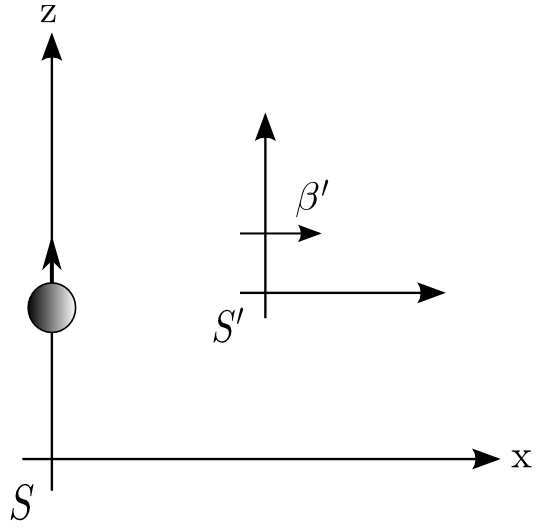
Figure 1: Lab frame $S$, and the boosted frame $S^{\prime}$

$$L(p)_{\hat{z}}=\begin{pmatrix}\gamma&0&0&\sqrt{\gamma^{2}-1}\\ 0&1&0&0\\ 0&0&1&0\\ \sqrt{\gamma^{2}-1}&0&0&\gamma\end{pmatrix}$$ (92)

where $\gamma$ is the rapidity and the $\Lambda_{\hat{x}}$ is

$$\Lambda_{\hat{x}}=\begin{pmatrix}\cosh{\alpha}&\sinh{\alpha}&0&0\\ \sinh{\alpha}&\cosh{\alpha}&0&0\\ 0&0&1&0\\ 0&0&0&1\end{pmatrix}$$ (93)

where $\cosh{\alpha}=\gamma^{\prime}$ and $\sinh{\alpha}=-\gamma^{\prime}\beta^{\prime}$.

Then the Wigner rotation can be obtained as,

$$L(\Lambda p)=\Lambda_{\hat{x}}L(p)_{\hat{z}}W_{-\hat{y}}^{-1}(\theta_{W})=$$ (94)

$$\begin{pmatrix}\cosh{\alpha}&\sinh{\alpha}&0&0\\ \sinh{\alpha}&\cosh{\alpha}&0&0\\ 0&0&1&0\\ 0&0&0&1\end{pmatrix}\begin{pmatrix}\gamma&0&0&\sqrt{\gamma^{2}-1}\\ 0&1&0&0\\ 0&0&1&0\\ \sqrt{\gamma^{2}-1}&0&0&\gamma\end{pmatrix}\begin{pmatrix}1&0&0&0\\ 0&\cos{\theta_{W}}&0&\sin{\theta_{W}}\\ 0&0&1&0\\ 0&-\sin{\theta_{W}}&0&\cos{\theta_{W}}\end{pmatrix}=$$

$$\begin{pmatrix}\gamma\cosh{\alpha}&\sinh{\alpha}\cos{\theta_{W}}+\sqrt{\gamma^{2}-1}\sin{\theta_{W}}\cosh{\alpha}&0&-\sinh{\alpha}\sin{\theta_{W}}+\sqrt{\gamma^{2}-1}\cos{\theta_{W}}\cosh{\alpha}\\ \gamma\sinh{\alpha}&\sqrt{\gamma^{2}-1}\sinh{\alpha}\sin{\theta_{W}}+\cos{\theta_{W}}\cosh{\alpha}&0&-\cosh{\alpha}\sin{\theta_{W}}+\sqrt{\gamma^{2}-1}\cos{\theta_{W}}\sinh{\alpha}\\ 0&0&1&0\\ \sqrt{\gamma^{2}-1}&\gamma\sin{\theta_{W}}&0&\gamma\cos{\theta_{W}}\end{pmatrix}.$$

From symmetry of the boost matrix, we have

$$\gamma\sin{\theta_{W}}=-\cosh{\alpha}\sin{\theta_{W}}+\sqrt{\gamma^{2}-1}\cos{\theta_{W}}\sinh{\alpha}.$$

Thus we can determine the Wigner angle as,

$$\tan{\theta_{W}}=\dfrac{\sinh{\alpha}\sqrt{\gamma^{2}-1}}{\gamma+\cosh{\alpha}}=\dfrac{-\gamma^{\prime}\gamma\beta^{\prime}\beta}{\gamma^{\prime}+\gamma}.$$ (95)

Finally, spin-$\frac{1}{2}$ representation of $W(\theta_{W})$ is

$$D^{s=1/2}(\theta_{W}) = 1\cos{\frac{\theta_{W}}{2}}+i(\mathbf{\sigma}\cdot\hat{n})\sin{\frac{\theta_{W}}{2}}$$ (96)

$$= 1\cos{\frac{\theta_{W}}{2}}-i(\sigma_{y})\sin{\frac{\theta_{W}}{2}}$$ (97)

$$= \begin{pmatrix}D^{1/2}_{\sigma^{\prime}=\frac{1}{2}\sigma=\frac{1}{2}}&D^{1/2}_{\sigma^{\prime}=\frac{1}{2}\sigma=-\frac{1}{2}}\\ D^{1/2}_{\sigma^{\prime}=-\frac{1}{2}\sigma=\frac{1}{2}}&D^{1/2}_{\sigma^{\prime}=-\frac{1}{2}\sigma=-\frac{1}{2}}\end{pmatrix}=\begin{pmatrix}\cos{\frac{\theta_{W}}{2}}&-\sin{\frac{\theta_{W}}{2}}\\ \sin{\frac{\theta_{W}}{2}}&\cos{\frac{\theta_{W}}{2}}\end{pmatrix}$$ (98)

where $\hat{n}$ is the direction of the rotation which is $\hat{e}\times\hat{p}$, in our case it is $\hat{x}\times\hat{z}=-\hat{y}$.

One can find the spin-up state in the $S^{\prime}$-frame. Firstly, spin-up state can be constructed as

$$|\uparrow\rangle=a^{\dagger}(p,\frac{1}{2})|0\rangle.$$ (99)

We have previously found the transformation rule for the massive particle as

$$U(\Lambda)|\uparrow\rangle = U(\Lambda)a^{\dagger}(p,\frac{1}{2})U^{-1}(\Lambda)U(\Lambda)|0\rangle=U(\Lambda)a^{\dagger}(p,\frac{1}{2})U^{-1}(\Lambda)|0\rangle$$ (100)

$$= \sqrt{\dfrac{(\Lambda p)^{0}}{p^{0}}}\sum_{\sigma^{\prime}}D^{s}_{\sigma^{\prime}\frac{1}{2}}(\theta_{W})a^{\dagger}(\Lambda p,\sigma^{\prime})|0\rangle.$$

Thus

$$U(\Lambda)|p,\frac{1}{2}\rangle = \sqrt{\dfrac{(\Lambda p)^{0}}{p^{0}}}\left(D^{1/2}_{\frac{1}{2}\frac{1}{2}}(\theta_{W})a^{\dagger}(\Lambda p,\frac{1}{2})+D^{1/2}_{-\frac{1}{2}\frac{1}{2}}(\theta_{W})a^{\dagger}(\Lambda p,-\frac{1}{2})\right)|0\rangle$$ (101)

$$= \sqrt{\dfrac{(\Lambda p)^{0}}{p^{0}}}\left(\cos{\frac{\theta_{W}}{2}}|\Lambda p,\frac{1}{2}\rangle+\sin{\frac{\theta_{W}}{2}}|\Lambda p,-\frac{1}{2}\rangle\right)$$

where $\dfrac{(\Lambda p)^{0}}{p^{0}}=\gamma^{\prime}$, $\theta_{W}=\arctan(\frac{-\gamma^{\prime}\gamma\beta^{\prime}\beta}{\gamma^{\prime}+\gamma})$, and

$$\Lambda\mathbf{p}=m\left(-\gamma^{\prime}\gamma\beta^{\prime}\hat{i}+\beta\gamma\hat{k}\right).$$ (102)

III ENTANGLEMENT

Entanglement is the most distinctive feature of quantum mechanics that certainly differentiates it from classical mechanics. Actually this amazing phenomenon is a manifestation of the non local character of the quantum theory. It was first introduced by A. Einstein, B. Podolsky, and N. Rosen as a thought experiment in 1935 epr to argue that quantum mechanics is not a complete physical theory. In time due to the works triggered by EPR, this issue grew into a new field of research activity. One of the milestones in this direction is the work of J.S. Bell who has shown that a local theory can not describe all the aspects of quantum mechanics bell . In this respect, entanglement must be discussed in the context of the question raised by EPR and the solution proposed by J.S. Bell.

III.1 Can Quantum Mechanical Description of Physical Reality Be Considered Complete?

Let’s briefly review this one of the most cited articles of human history. This article starts with the discussion and definition of “complete theory” and “condition of reality”. They define a complete theory as any physical theory must include all the elements of physical reality, on the other hand the condition of reality is described as predicting physical quantity in a certain way without disturbing the system. However in quantum mechanics, incompatible observables can not be simultaneously measured. As a result, either the quantum mechanical description of physical realty is not complete, or the values of the incompatible observables can not be simultaneously real. If the quantum mechanics is a complete theory then second argument is correct.

Consider two particles with a space-like separation. In quantum mechanics, one can define the wave function of the composite system as

$$\Psi(x_{1},x_{2})=\sum_{n=1}^{\infty}\psi_{n}(x_{2})u_{n}(x_{1})$$ (103)

where $u_{n}(x_{1})$ is the wave function of the first particle which is the eigenfunction of some operator $A$ with the corresponding eigenvalue $a_{n}$, and $\psi_{n}(x_{2})$ is wave function of the second one. According to the measurement postulate of quantum mechanics, if the observable $A$ is measured on the first particle with the value $a_{k}$, then after the measurement the wave function of the first particle collapses to the $u_{k}(x_{1})$, and second one collapses to the $\psi_{k}(x_{2})$.

Alternatively, this physical function can be expanded in terms of the eigenfunctions of some different operator $B$, such that

$$\Psi(x_{1},x_{2})=\sum_{s=1}^{\infty}\phi_{s}(x_{2})v_{s}(x_{1}).$$ (104)

Then if the result of the measurement of $B$ is $b_{r}$ and corresponding collapsed function is $v_{r}(x_{1})$ for the first particle, then second particle automatically collapses to the $\phi_{r}(x_{2})$.

Furthermore, this process can be performed with the incompatible observables $A$ and $B$. The strange thing is that one can predict the physical values of $A$ and $B$ with certainty without disturbing the second particle, via a single measurement on the joint system.

Here, we have started our discussion by accepting quantum mechanics as a complete theory, however we have ended up with the result that contradicts it.

Then one can conclude naturally that quantum mechanical description of physical reality can not be considered complete. One resolution of the problem was based on the hidden variables.

Actually one of the most important aspect of that paper was the introduction of the entangled states. It was shown that this paradox occurs only in entangled states, and this phenomenon is known as “entanglement”. It was originally called by Schrödinger as “Verschrankung” schrodinger .

As one can see, the main assumption that lies in the background of EPR’s argument is the locality condition.

III.2 On the Einstein-Podolsky-Rosen paradox

In his analysis of the EPR problem, J.S. Bell uses the version of D. Bohm and Y. Aharonov bohm . This entangled state is a well known singlet state which is

$$|singlet\rangle=\dfrac{1}{\sqrt{2}}\left(|\hat{s};\uparrow\rangle|\hat{s};\downarrow\rangle-|\hat{s};\downarrow\rangle|\hat{s};\uparrow\rangle\right)$$ (105)

where $\hat{s}$ is the spin polarization direction.

In quantum mechanics, the correlation function for the singlet state is given by

$$C(\hat{a},\hat{b})=\langle singlet|\boldsymbol{\sigma}_{1}\cdot\hat{a}\;\boldsymbol{\sigma}_{2}\cdot\hat{b}|singlet\rangle=-\hat{a}\cdot\hat{b}.$$ (106)

To prove this, let us first note that

$$\boldsymbol{\sigma}_{1}|singlet\rangle=-\boldsymbol{\sigma}_{2}|singlet\rangle$$

then

$$\langle{\sigma_{1}}_{i}a_{i}{\sigma_{2}}_{j}b_{j}\rangle = -a_{i}b_{j}\langle{\sigma_{1}}_{i}{\sigma_{1}}_{j}\rangle$$

$$= -a_{i}b_{j}\langle\delta_{ij}+i\epsilon_{ijk}{\sigma_{1}}_{k}\rangle=-\hat{a}\cdot\hat{b}$$

where we used the fact that the expectation value of ${\sigma_{1}}_{k}$ is zero in the singlet state.

Let’s introduce a hidden variable $\lambda$ which can be anything such that the complicated measurement processes are determined by this parameter and also measurement direction. Let the result of the measurement of $\boldsymbol{\sigma}_{1}\cdot\hat{a}$ on the first particle and $\boldsymbol{\sigma}_{2}\cdot\hat{b}$ on the second particle be

$$A(\hat{a},\lambda)=\pm 1\quad\mbox{and}\quad B(\hat{b},\lambda)=\pm 1$$ (107)

respectively. The crucial point is that result on the first particle does not depend on $\hat{b}$ and vice versa. Then the correlation for the singlet state is given by

$$C(\hat{a},\hat{b})=\int d\lambda\rho(\lambda)A(\hat{a},\lambda)B(\hat{b},\lambda)$$ (108)

where $\rho(\lambda)$ is the probability distribution that depends on $\lambda$. This result has to match with the quantum mechanical result. But it is shown that this is impossible.

Before showing the contradiction, first it is easy to show how hidden variable theory can work on a single particle state and on a singlet state.

For the single particle state, let the hidden variable be a unit vector with uniform probability distribution over the hemisphere $\hat{\lambda}\cdot\hat{s}>0$, then the result of the measurement can be defined as

$$sign\;\hat{\lambda}\cdot\hat{a}^{\prime}$$ (109)

where unit vector $\hat{a}^{\prime}$ depends on $\hat{a}$ and $\hat{s}$. ( This result does not say anything about when $\hat{\lambda}\cdot\hat{a}^{\prime}$, however the probability of getting it is zero, $P(\hat{\lambda}\cdot\hat{a}^{\prime}=0)=0$.)

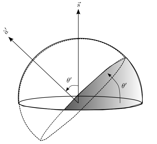
Figure 2: Single particle configuration

The expectation value for a single particle state in the spin polarization direction $\hat{s}$, is then

$$\langle\boldsymbol{\sigma}\cdot\hat{a}\rangle=1P(\hat{\lambda}\cdot\hat{a}^{\prime}>0)-1P(\hat{\lambda}\cdot\hat{a}^{\prime}<0)=1-\dfrac{2\theta^{\prime}}{\pi}$$ (110)

where $\theta^{\prime}$ is the angle between $\hat{a}^{\prime}$ and $\hat{\lambda}$ as shown in the figure (2). Then, $\theta^{\prime}$ can be adjusted such that

$$1-\dfrac{2\theta^{\prime}}{\pi}=\cos\theta$$ (111)

where $\theta$ is the angle between $\hat{a}$ and $\hat{s}$. Thus we have reached the desired result as in the quantum mechanics.

For the singlet state, it can be shown that

$$C(\hat{a},\hat{a}) = C(\hat{a},-\hat{a})=-1$$ (112)

$$C(\hat{a},\hat{b}) = 0\quad\mbox{for}\quad\hat{a}\cdot\hat{b}=0.$$

To show this, let $\lambda$ be a unit vector $\hat{\lambda}$, with uniform probability distribution over all directions, and

$$A(\hat{a},\hat{\lambda})=sign\;\hat{a}\cdot\hat{\lambda}$$ (113)

$$B(\hat{b},\hat{\lambda})=-sign\;\hat{b}\cdot\hat{\lambda}.$$

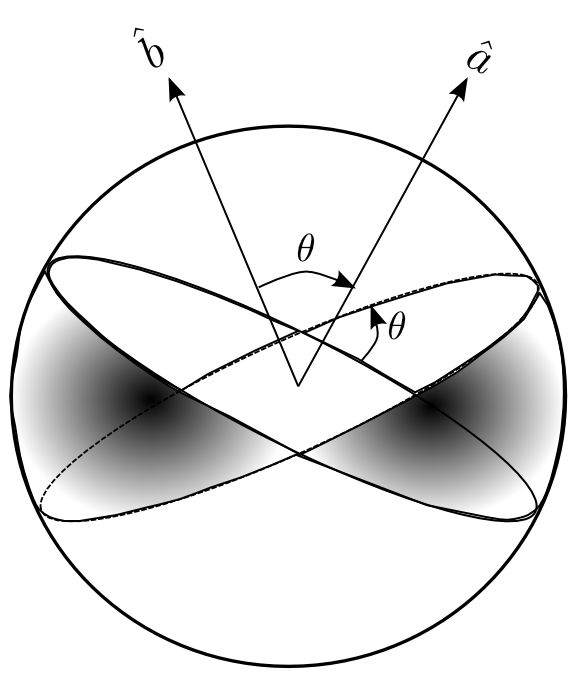
Figure 3: Singlet state configuration peres

Then one gets

$$C(\hat{a},\hat{b})=1P\left(\binom{\hat{a}\cdot\hat{\lambda}>0}{\hat{b}\cdot\hat{\lambda}<0}\,\mbox{or}\,\binom{\hat{a}\cdot\hat{\lambda}<0}{\hat{b}\cdot\hat{\lambda}>0}\right)-1P\left(\binom{\hat{a}\cdot\hat{\lambda}<0}{\hat{b}\cdot\hat{\lambda}<0}\,\mbox{or}\,\binom{\hat{a}\cdot\hat{\lambda}>0}{\hat{b}\cdot\hat{\lambda}>0}\right)=-1+\dfrac{2\theta}{\pi}$$ (114)

where $\theta$ is the angle between $\hat{a}$ and $\hat{b}$ as shown in the figure (3). This equation satisfies (112).

Furthermore one can reproduce the quantum mechanical value in (106), by allowing that the result of the measurement on each particle depend also on the measurement direction of the other particle corresponding the replacement of $\hat{a}$ with $\hat{a}^{\prime}$, which is obtained from $\hat{a}$ by rotating towards $\hat{b}$ until

$$C(\hat{a},\hat{b})=-1+\dfrac{2\theta^{\prime}}{\pi}=-\cos\theta$$ (115)

holds, where $\theta^{\prime}$ is the angle between $\hat{a}^{\prime}$ and $\hat{b}$. However we can not permit this since we are looking for a local theory.

Next we turn our attention to comparing the hidden variable theory and quantum mechanics. To show the contradictions between the result of local hidden variable theory and the quantum mechanics, we proceed as follows:

Since $\rho$ is normalized, we have

$$\int d\lambda\rho(\lambda)=1$$ (116)

and for the singlet state

$$A(\hat{a},\lambda)=-B(\hat{a},\lambda).$$ (117)

Then (108) can be written as

$$C(\hat{a},\hat{b})=-\int d\lambda\rho(\lambda)A(\hat{a},\lambda)A(\hat{b},\lambda).$$ (118)

Next, we introduce another unit vector $\hat{c}$, and consider

$$C(\hat{a},\hat{b})-C(\hat{a},\hat{c}) = -\int d\lambda\rho(\lambda)\left(A(\hat{a},\lambda)A(\hat{b},\lambda)-A(\hat{a},\lambda)A(\hat{c},\lambda)\right)$$

$$= \int d\lambda\rho(\lambda)A(\hat{a},\lambda)A(\hat{b},\lambda)\left(A(\hat{b},\lambda)A(\hat{c},\lambda)-1\right)$$

where we have used the fact that $[A(\hat{b},\lambda)]^{2}=1$. Since $A(\hat{a},\lambda)=\pm 1$, this equation can be written as

$$|C(\hat{a},\hat{b})-C(\hat{a},\hat{c})|\leq\int d\lambda\rho(\lambda)\left(1-A(\hat{b},\lambda)A(\hat{c},\lambda)\right)$$ (120)

then finally we get

$$1+C(\hat{b},\hat{c})\geq|C(\hat{a},\hat{b})-C(\hat{a},\hat{c})|$$ (121)

This is the original form of famous Bell inequality.

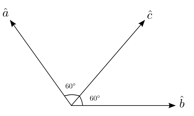
Figure 4: Angles that violates the Bell inequality

It is easy to show that for some special directions this inequality can not be satisfied by the quantum mechanical result. The Bell inequality (121) for the quantum mechanics becomes

$$1-\cos(\theta_{bc})\geq|\cos(\theta_{ab})-\cos(\theta_{ac})|.$$ (122)

One can easily see that this is not satisfied for the angles shown in figure (4).

As a result, introducing a variable to account for the measurement process does not correspond to the right statistical behavior of quantum mechanics. However as in the case of (115), if the measurement result of one of the entangled pair depends also on the measurement of the other, then it meets the quantum mechanical criteria. Then this hidden variable must propagate instantaneously, but such a theory can not be Lorentz invariant.
Thus, the question asked by EPR is solved by J. S. Bell and this solution has been verified by A. Aspect in a series of experiments aspect .

III.3 Definition of Entanglement

After the discussion on the two historically important papers, one can describe the entanglement in terms of the postulates of quantum mechanics. According to Postulate 4, total Hilbert space of the composite system is formed by tensor product of Hilbert spaces of subsystems. In that total space, there are such states that can not be written as a tensor product of states representing the subsystem.

Consider an n-partite composite system, and

$$|\psi_{i}\rangle\in\mathcal{H}_{i}\quad\mbox{where}\quad i=1,2,3,\cdots,n$$ (123)

Then there are states in the $\mathcal{H}=\bigotimes_{i=1}^{n}\mathcal{H}_{i}$ such that

$$|\psi\rangle\neq\bigotimes_{i=1}^{n}|\psi_{i}\rangle.$$ (124)

These states are called entangled states. Any state that is not entangled is called separable.

In this work, we only concentrate on bipartite states.

III.3.1 Bipartite Entanglement

Consider two quantum systems, the first one is owned by Alice, and the second one by Bob. Alice’s system may be described by states in a Hilbert space $\mathcal{H}_{A}$ of dimension N and Bob’s one $\mathcal{H}_{B}$ of dimension M. The composite system of both parties is then described by the vectors in the tensor-product form of the two spaces $\mathcal{H}=\mathcal{H}_{A}\otimes\mathcal{H}_{B}$.

Let $|a_{i}\rangle$ be a basis of Alice’s space and $|b_{j}\rangle$ be basis of Bob’s space. Then in $\mathcal{H}_{A}\otimes\mathcal{H}_{B}$ we have the set of all linear combinations of the states $|a_{i}\rangle\otimes|b_{j}\rangle$ to be used as bases. Thus any state in $\mathcal{H}_{A}\otimes\mathcal{H}_{B}$ can be written as

$$|\psi\rangle=\sum_{i,j=1}^{N,M}c_{ij}|a_{i}\rangle\otimes|b_{j}\rangle\,\in\mathcal{H}_{A}\otimes\mathcal{H}_{B}$$ (125)

with a complex $N\times M$ matrix $C=(c_{ij})$.

The measurement of observables can be defined in a similar way, if A is an observable on Alice’s space and B on Bob’s space, the expectation value of $A\otimes B$ is defined as

$$\langle\psi|(A\otimes B)|\psi\rangle=\sum_{i,j=1}^{N,M}\sum_{i^{\prime},j^{\prime}=1}^{N,M}c_{ij}^{*}c_{i^{\prime}j^{\prime}}\langle a_{i}|A|a_{i^{\prime}}\rangle\langle b_{j}|B|b_{j^{\prime}}\rangle.$$ (126)

Now we can define separability and entanglement for these states. A pure state $|\psi\rangle\in\mathcal{H}$ is called a “product state” or “separable” if one can find states $|\phi^{A}\rangle\in\mathcal{H}_{A}$ and $|\phi^{B}\rangle\in\mathcal{H}_{B}$ such that $|\psi\rangle=|\phi^{A}\rangle\otimes|\phi^{B}\rangle$ holds. Otherwise the state $|\psi\rangle$ is called entangled.

Physically, the definition of product state means that the state is uncorrelated. Thus a product state can be prepared in a local way. In other word Alice produces the state $|\phi^{A}\rangle$ and Bob does independently $|\phi^{B}\rangle$. If Alice measures any observable A and Bob measures B, the measurement outcomes for Alice do not depend on the outcomes on Bob’s side.

In a pure state, it is easy to decide whether a given pure state is entangled or not. $|\psi\rangle$ is a product state, if and only if the rank of the matrix $C=(c_{ij})$ in (125) equals one. This is due to the fact that a matrix C is of rank one, if and only if there exist two vectors a and b such that $c_{ij}=a_{i}b_{j}$. So one can write

$$|\psi\rangle=\left(\sum_{i}a_{i}|a_{i}\rangle\right)\otimes\left(\sum_{j}b_{j}|b_{j}\rangle\right)$$ (127)

which means that it is the product state. Another important tool for the description of entanglement for bipartite systems only is the Schmidt decomposition, we turn our attention next:

Let $|\psi\rangle=\sum_{i,j=1}^{N,M}c_{ij}|a_{i}b_{j}\rangle\,\in\mathcal{H}_{A}\otimes\mathcal{H}_{B}$ be a vector in the tensor product space of the two Hilbert spaces. Then there exists an orthonormal basis $|i\rangle_{A}$ of $\mathcal{H}_{A}$ and an orthonormal basis $|i\rangle_{B}$ of $\mathcal{H}_{B}$ such that

$$|\psi\rangle=\sum_{i=1}^{R}\lambda_{i}|i\rangle_{A}\otimes|i\rangle_{B}$$ (128)

holds, with positive real coefficients $\lambda_{i}$. The $\lambda_{i}$’s are the square roots of eigenvalues of matrix, $CC^{\dagger}$ where $C=(c_{ij})$, and are called the Schmidt coefficients. The number $R=\min(dim(\mathcal{H}_{A}),dim(\mathcal{H}_{B}))$ is called the Schmidt Rank/Number of $|\psi\rangle$. If R equals one then, the state is product state, otherwise it is entangled. For an entangled state, if the absolute values of all non vanishing Schmidt coefficients are the same, then it is called maximally entangled state.

III.3.2 von Neumann Entropy

It is worth pointing out that from Schmidt form one can define the von Neumann entropy which can be used as a measure of entanglement, as

$$S=-\sum_{j}|\lambda_{j}|^{2}\log_{2}|\lambda_{j}|^{2}.$$ (129)

From this definition, one can easily observe that if a given state is a product state which means that the Schmidt rank is equal to one in the spectral decomposition, then the von Neumann entropy is zero. However for an entangled state, the von Neumann entropy never vanishes. Furthermore, for a maximally entangled state, the von Neumann entropy is

$$S=\log_{2}(R)$$ (130)

where $R>1$.

III.3.3 Bell States

An important set of entangled states are the Bell states, which are maximally entangled states.

$$|\psi^{+}\rangle=\dfrac{1}{\sqrt{2}}(|01\rangle+|10\rangle) |\phi^{+}\rangle=\dfrac{1}{\sqrt{2}}(|00\rangle+|11\rangle)$$ (131)

$$|\psi^{-}\rangle=\dfrac{1}{\sqrt{2}}(|01\rangle-|10\rangle) |\phi^{-}\rangle=\dfrac{1}{\sqrt{2}}(|00\rangle-|11\rangle).$$

They form an orthonormal basis on the composite Hilbert space of bipartite system, in the sense that any other state in this space can be produced from each of them by local operations. Since the Bell states are already in the Schmidt form, one can find the von Neumann entropy of these states by using (130) as

$$S=1.$$ (132)

III.4 CHSH Inequality

Bell inequality in (121) can be written in a more elegant way. For a bipartite system, consider four dichotomous operators $Q$, $R$, $S$, and $T$ which can take the values $\pm 1$. Let $Q$ and $R$ be defined on the one system, $S$ and $T$ be on the other system, then with these four operator one can write such an equation that

$$(Q+R)S+(Q-R)T=\pm 2$$ (133)

always holds. Average of this equation leads to an inequality

$$|\langle(Q+R)S+(Q-R)T\rangle|\leq 2.$$ (134)

It is the well known CHSH inequality chsh . This inequality states that any local theory must satisfy it. However in quantum mechanics, expectation value of certain observables for the entangled states violates this inequality as follows:

Consider the singlet state

$$|singlet\rangle=\dfrac{1}{\sqrt{2}}\left(|\hat{s};\uparrow\rangle|\hat{s};\downarrow\rangle-|\hat{s};\downarrow\rangle|\hat{s};\uparrow\rangle.\right)$$ (135)

Since the singlet state is an entangled state in the spin degree of freedom, (134) can be written in terms of correlation functions as

$$|C(\hat{a},\hat{b})+C(\hat{a^{\prime}},\hat{b})+C(\hat{a^{\prime}},\hat{b^{\prime}})-C(\hat{a},\hat{b^{\prime}})|\leq 2$$ (136)

where $\hat{a}$, $\hat{b}$, $\hat{a^{\prime}}$, and $\hat{b^{\prime}}$ are the spin measurement directions. If one chooses the $\hat{a}$, $\hat{b}$, $\hat{a^{\prime}}$, and $\hat{b^{\prime}}$ as

$$\hat{a} = (0,0,1)$$

$$\hat{b} = (1/\sqrt{2},0,1/\sqrt{2})$$

$$\hat{a^{\prime}} = (1,0,0)$$

$$\hat{b^{\prime}} = (1/\sqrt{2},0,-1/\sqrt{2})$$

then CHSH inequality for the singlet state gives

$$|C(\hat{a},\hat{b})+C(\hat{a^{\prime}},\hat{b})+C(\hat{a^{\prime}},\hat{b^{\prime}})-C(\hat{a},\hat{b^{\prime}})|=2\sqrt{2}.$$ (137)

This is the verification of the non local character of quantum mechanics. CHSH inequality is valid for the bipartite systems and any bipartite entangled state violates this inequality in certain directions.

Furthermore one can find the upper limit of this inequality. Since these four operator are dichotomous, square of these operators are equal to identity operator. As a result, one can find

$$\left[(Q+R)S+(Q-R)T\right]^{2}=4I-[Q,R]\otimes[S,T].$$ (138)

Then, taking the expectation value, and using the Schwarz’s Inequality, one can obtain

$$|\langle(Q+R)S+(Q-R)T\rangle|\leq\sqrt{4-\langle[Q,R]\otimes[S,T]\rangle}.$$ (139)

This is the quantum generalization of Bell-type inequality tsirelson . One can find that upper limit for the CHSH inequality is $2\sqrt{2}$. As a result, (137) is the maximum violation of the inequality.

IV LORENTZ TRANSFORMATION OF ENTANGLED STATES AND BELL INEQUALITY

IV.1 Transformation of Entangled States

In this thesis, we have only been interested in the transformation of the Bell states. Consider a frame, $S$ which observes the four momenta of the particles as $p_{1}$ and $p_{2}$, respectively. In terms of the creation operators, these four states can be written in this frame as,

$$|\Phi^{\pm}\rangle = \dfrac{1}{\sqrt{2}}\left(a^{\dagger}(p_{1},\frac{1}{2})a^{\dagger}(p_{2},\frac{1}{2})\pm a^{\dagger}(p_{1},-\frac{1}{2})a^{\dagger}(p_{2},-\frac{1}{2})\right)|0\rangle$$ (140)

$$|\Psi^{\pm}\rangle = \dfrac{1}{\sqrt{2}}\left(a^{\dagger}(p_{1},\frac{1}{2})a^{\dagger}(p_{2},-\frac{1}{2})\pm a^{\dagger}(p_{1},-\frac{1}{2})a^{\dagger}(p_{2},\frac{1}{2})\right)|0\rangle.$$ (141)

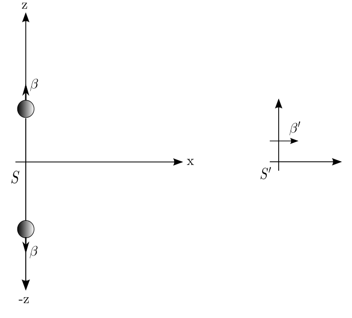
Figure 5: Zero momentum and boosted frame.

For simplicity, these two particles can be taken as identical and $S$ frame can be chosen as the zero momentum frame which means, $\mathbf{p}_{1}=-\mathbf{p}_{2}=\mathbf{p}=\gamma\beta m\hat{z}$ and also $p_{1}^{0}=p_{2}^{0}$. Define another frame $S^{\prime}$ which is boosted in the positive $\hat{x}$ direction relative to the $S$-frame.

We will now work out the transformation of these states to the frame $S^{\prime}$. First of all, we have to determine the Wigner angles for both particles. For the first particle $D^{s=1/2}_{1}(\theta_{W})$ is given by (98) and the Wigner angle, $\theta_{W}$ is in (95). For the second particle since $L(p)_{-\hat{z}}$ in the $-z$-direction, the Wigner rotation is about the $+y$-direction, but the angle is not changed, so

$$D^{s=1/2}_{2}(\theta_{W})=\begin{pmatrix}\cos{\frac{\theta_{W}}{2}}&\sin{\frac{\theta_{W}}{2}}\\ -\sin{\frac{\theta_{W}}{2}}&\cos{\frac{\theta_{W}}{2}}\end{pmatrix}.$$ (142)

However transformed momenta are not the same. We will keep it as $(\Lambda(-\mathbf{p}))$ and it is given by

$$L(\Lambda-p)=\Lambda_{\hat{x}}L(p)_{-\hat{z}}W_{\hat{y}}^{-1}(\theta_{W})=$$ (143)

$$\begin{pmatrix}\cosh{\alpha}&\sinh{\alpha}&0&0\\ \sinh{\alpha}&\cosh{\alpha}&0&0\\ 0&0&1&0\\ 0&0&0&1\end{pmatrix}\begin{pmatrix}\gamma&0&0&-\sqrt{\gamma^{2}-1}\\ 0&1&0&0\\ 0&0&1&0\\ -\sqrt{\gamma^{2}-1}&0&0&\gamma\end{pmatrix}\begin{pmatrix}1&0&0&0\\ 0&\cos{\theta_{W}}&0&-\sin{\theta_{W}}\\ 0&0&1&0\\ 0&\sin{\theta_{W}}&0&\cos{\theta_{W}}\end{pmatrix}=$$

$$\begin{pmatrix}\gamma\cosh{\alpha}&\sinh{\alpha}\cos{\theta_{W}}+\sqrt{\gamma^{2}-1}\sin{\theta_{W}}\cosh{\alpha}&0&\sinh{\alpha}\sin{\theta_{W}}-\sqrt{\gamma^{2}-1}\cos{\theta_{W}}\cosh{\alpha}\\ \gamma\sinh{\alpha}&\sqrt{\gamma^{2}-1}\sinh{\alpha}\sin{\theta_{W}}+\cos{\theta_{W}}\cosh{\alpha}&0&\cosh{\alpha}\sin{\theta_{W}}-\sqrt{\gamma^{2}-1}\cos{\theta_{W}}\sinh{\alpha}\\ 0&0&1&0\\ -\sqrt{\gamma^{2}-1}&-\gamma\sin{\theta_{W}}&0&\gamma\cos{\theta_{W}}\end{pmatrix}.$$

Next, we will find the $|\Phi^{+}\rangle$ in the $S^{\prime}$-frame,

$$U(\Lambda)|\Phi^{+}\rangle = \dfrac{1}{\sqrt{2}}\left(U(\Lambda)a^{\dagger}(\mathbf{p},\frac{1}{2})U^{-1}(\Lambda)U(\Lambda)a^{\dagger}(-\mathbf{p},\frac{1}{2})U^{-1}(\Lambda)U(\Lambda)\right)|0\rangle$$

$$+ \dfrac{1}{\sqrt{2}}\left(U(\Lambda)a^{\dagger}(\mathbf{p},-\frac{1}{2})U^{-1}(\Lambda)U(\Lambda)a^{\dagger}(-\mathbf{p},-\frac{1}{2})U^{-1}(\Lambda)U(\Lambda)\right)|0\rangle.$$

Using the transformation properties of the creation operator, we get

$$U(\Lambda)|\Phi^{+}\rangle = \dfrac{1}{\sqrt{2}}\dfrac{(\Lambda p)^{0}}{p^{0}}\sum_{\sigma^{\prime},\sigma^{\prime\prime}}\left({D^{s}_{1}}_{\sigma^{\prime}\frac{1}{2}}(\theta_{W})a^{\dagger}(\Lambda\mathbf{p},\sigma^{\prime}){D^{s}_{2}}_{\sigma^{\prime\prime}\frac{1}{2}}(\theta_{W})a^{\dagger}(\Lambda(-\mathbf{p}),\sigma^{\prime\prime})\right)|0\rangle$$

$$+ \dfrac{1}{\sqrt{2}}\dfrac{(\Lambda p)^{0}}{p^{0}}\sum_{\sigma^{\prime},\sigma^{\prime\prime}}\left({D^{s}_{1}}_{\sigma^{\prime}-\frac{1}{2}}(\theta_{W})a^{\dagger}(\Lambda\mathbf{p},\sigma^{\prime}){D^{s}_{2}}_{\sigma^{\prime\prime}-\frac{1}{2}}(\theta_{W})a^{\dagger}(\Lambda(-\mathbf{p}),\sigma^{\prime\prime})\right)|0\rangle.$$

Now using the spin-$s$ representation of rotations

$$U(\Lambda)|\Phi^{+}\rangle =\dfrac{1}{\sqrt{2}}\dfrac{(\Lambda p)^{0}}{p^{0}}\bigg{(}\cos^{2}{\frac{\theta_{W}}{2}}a^{\dagger}(\Lambda\mathbf{p},\frac{1}{2})a^{\dagger}(\Lambda(-\mathbf{p}),\frac{1}{2})-\cos{\frac{\theta_{W}}{2}}\sin{\frac{\theta_{W}}{2}}a^{\dagger}(\Lambda\mathbf{p},\frac{1}{2})a^{\dagger}(\Lambda(-\mathbf{p}),-\frac{1}{2})$$

$$+\cos{\frac{\theta_{W}}{2}}\sin{\frac{\theta_{W}}{2}}a^{\dagger}(\Lambda\mathbf{p},-\frac{1}{2})a^{\dagger}(\Lambda(-\mathbf{p}),\frac{1}{2})-\sin^{2}{\frac{\theta_{W}}{2}}a^{\dagger}(\Lambda\mathbf{p},-\frac{1}{2})a^{\dagger}(\Lambda(-\mathbf{p}),-\frac{1}{2})$$

$$-\sin^{2}{\frac{\theta_{W}}{2}}a^{\dagger}(\Lambda\mathbf{p},\frac{1}{2})a^{\dagger}(\Lambda(-\mathbf{p}),\frac{1}{2})-\cos{\frac{\theta_{W}}{2}}\sin{\frac{\theta_{W}}{2}}a^{\dagger}(\Lambda\mathbf{p},\frac{1}{2})a^{\dagger}(\Lambda(-\mathbf{p}),-\frac{1}{2})$$

$$+\cos{\frac{\theta_{W}}{2}}\sin{\frac{\theta_{W}}{2}}a^{\dagger}(\Lambda\mathbf{p},-\frac{1}{2})a^{\dagger}(\Lambda(-\mathbf{p}),\frac{1}{2})+\cos^{2}{\frac{\theta_{W}}{2}}a^{\dagger}(\Lambda\mathbf{p},-\frac{1}{2})a^{\dagger}(\Lambda(-\mathbf{p}),-\frac{1}{2})\bigg{)}|0\rangle$$

one can obtain

$$U(\Lambda)|\Phi^{+}\rangle =\dfrac{1}{\sqrt{2}}\dfrac{(\Lambda p)^{0}}{p^{0}}\bigg{(}\cos{\theta_{W}}a^{\dagger}(\Lambda\mathbf{p},\frac{1}{2})a^{\dagger}(\Lambda(-\mathbf{p}),\frac{1}{2})-\sin{\theta_{W}}a^{\dagger}(\Lambda\mathbf{p},\frac{1}{2})a^{\dagger}(\Lambda(-\mathbf{p}),-\frac{1}{2})$$

$$+\sin{\theta_{W}}a^{\dagger}(\Lambda\mathbf{p},-\frac{1}{2})a^{\dagger}(\Lambda(-\mathbf{p}),\frac{1}{2})+\cos{\theta_{W}}a^{\dagger}(\Lambda\mathbf{p},-\frac{1}{2})a^{\dagger}(\Lambda(-\mathbf{p}),-\frac{1}{2})\bigg{)}|0\rangle.$$

Finally, this can be written as

$$U(\Lambda)|\Phi^{+}\rangle=\cos{\theta_{W}}|\Phi^{+}\rangle^{\prime}-\sin{\theta_{W}}|\Psi^{-}\rangle^{\prime}.$$ (144)

Similarly, one can find the transformation properties of the other Bell states as

$$U(\Lambda)|\Phi^{-}\rangle =|\Phi^{-}\rangle^{\prime}$$ (145)

$$U(\Lambda)|\Psi^{+}\rangle =|\Psi^{+}\rangle^{\prime}$$ (146)

$$U(\Lambda)|\Psi^{-}\rangle =\sin{\theta_{W}}|\Phi^{+}\rangle^{\prime}+\cos{\theta_{W}}|\Psi^{-}\rangle^{\prime}$$ (147)

where $\theta_{W}=\arctan(\frac{-\gamma^{\prime}\gamma\beta^{\prime}\beta}{\gamma^{\prime}+\gamma})$,

$$|\Phi^{\pm}\rangle^{\prime} = \dfrac{(\Lambda p)^{0}}{p^{0}}\dfrac{1}{\sqrt{2}}\left(a^{\dagger}(\Lambda\mathbf{p},\frac{1}{2})a^{\dagger}(\Lambda(-\mathbf{p}),\frac{1}{2})\pm a^{\dagger}(\Lambda\mathbf{p},-\frac{1}{2})a^{\dagger}(\Lambda(-\mathbf{p}),-\frac{1}{2})\right)|0\rangle$$ (148)

$$|\Psi^{\pm}\rangle^{\prime} = \dfrac{(\Lambda p)^{0}}{p^{0}}\dfrac{1}{\sqrt{2}}\left(a^{\dagger}(\Lambda\mathbf{p},\frac{1}{2})a^{\dagger}(\Lambda(-\mathbf{p}),-\frac{1}{2})\pm a^{\dagger}(\Lambda\mathbf{p},-\frac{1}{2})a^{\dagger}(\Lambda(-\mathbf{p}),\frac{1}{2})\right)|0\rangle$$ (149)

and

$$\Lambda(\pm\mathbf{p})=m\left(-\gamma^{\prime}\gamma\beta^{\prime}\hat{i}\pm\beta\gamma\hat{k}\right),\quad\dfrac{(\Lambda p)^{0}}{p^{0}}=\gamma^{\prime}.$$ (150)

After these discussions it is obvious that entanglement is a Lorentz invariant property. No inertial observer can see an entangled state as a product state.

This property can be proven in a general way starting from Schmidt form for bipartite states, which is presented in the following section.

IV.2 Schmidt Decomposition and Its Covariance

Consider two particles $A$ and $B$. The total state vector of the composite system can be decomposed as

$$|\psi\rangle=\sum_{i=1}^{R}{\lambda}_{i}{|i\rangle}_{A}\otimes{|i\rangle}_{B}$$ (151)

where ${\lambda}_{i}$ are the Schmidt coefficients, $R=\min(dim(\mathcal{H}_{A}),dim(\mathcal{H}_{B}))$ is the Schmidt rank and ${|i\rangle}_{A}$ and ${|i\rangle}_{B}$ are the orthonormal basis of the corresponding Hilbert spaces. These basis can be normalized as

$${}_{A}\langle i|j\rangle_{A} = \delta(\mathbf{p^{\prime}}_{A}-\mathbf{p}_{A})\delta_{ij}$$ (152)

$${}_{B}\langle i|j\rangle_{B} = \delta(\mathbf{p^{\prime}}_{B}-\mathbf{p}_{B})\delta_{ij}$$

where $\mathbf{p}_{A}$ and $\mathbf{p}_{B}$ momenta of the particles $A$ and $B$, respectively. Therefore, the normalization of the state vector of the composite system becomes

$$\langle\psi|\psi\rangle=\delta(\mathbf{p^{\prime}}_{A}-\mathbf{p}_{A})\delta(\mathbf{p^{\prime}}_{B}-\mathbf{p}_{B})$$ (153)

with the condition $\sum_{i}|\lambda_{i}|^{2}=1$.

The orthonormal basis ${|i\rangle}_{A}$ and ${|i\rangle}_{B}$ can be expanded in terms of the one particle states as the following

$$|i\rangle_{A} = \sum_{n=-s_{A}}^{s_{A}}A_{n}^{(i)}|p_{A},n\rangle$$ (154)

$$|i\rangle_{B} = \sum_{m=-s_{B}}^{s_{B}}B_{m}^{(i)}|p_{B},m\rangle$$

where $s_{A}$ and $s_{B}$ are the spins of the particles, respectively. As a result for this configuration, $R=\min(2s_{A}+1,2s_{B}+1)$.

Since these basis should satisfy (152),

$$\sum_{n=-s_{A}}^{s_{A}}{A}_{n}^{*(j)}{A}_{n}^{(i)}\delta(\mathbf{p^{\prime}}_{A}-\mathbf{p}_{A})=\delta(\mathbf{p^{\prime}}_{A}-\mathbf{p}_{A})\delta_{ij}$$ (155)

$$\sum_{m=-s_{B}}^{s_{B}}{B}_{m}^{*(j)}{B}_{m}^{(i)}\delta(\mathbf{p^{\prime}}_{B}-\mathbf{p}_{B})=\delta(\mathbf{p^{\prime}}_{B}-\mathbf{p}_{B})\delta_{ij}$$

must hold. Then, the Schmidt decomposition becomes

$$|\psi\rangle=\sum_{i=1}^{R}{\lambda}_{i}\sum_{n=-s_{A}}^{s_{A}}\sum_{m=-s_{B}}^{s_{B}}A_{n}^{(i)}B_{m}^{(i)}|p_{A},n\rangle\otimes|p_{B},m\rangle.$$

The one particle states can be written in terms of the creation operators as

$$|p_{A},n\rangle = a^{{\dagger}}(p_{A},n)|0\rangle$$

$$|p_{B},m\rangle = a^{{\dagger}}(p_{B},m)|0\rangle$$

where $|0\rangle$ is the Lorentz invariant vacuum state. Finally we get the Schmidt decomposition in terms of the creation operators as

$$|\psi\rangle=\sum_{i=1}^{R}{\lambda}_{i}\sum_{n=-s_{A}}^{s_{A}}\sum_{m=-s_{B}}^{s_{B}}A_{n}^{(i)}B_{m}^{(i)}a^{{\dagger}}(p_{A},n)a^{{\dagger}}(p_{B},m)|0\rangle.$$

Now we can apply Lorentz transformation on our state ket by the unitary transformation $U(\Lambda)$

$$U(\Lambda)|\psi\rangle=\sum_{i=1}^{R}{\lambda}_{i}\sum_{n=-s_{A}}^{s_{A}}\sum_{m=-s_{B}}^{s_{B}}A_{n}^{(i)}B_{m}^{(i)}U(\Lambda)a^{{\dagger}}(p_{A},n)U^{-1}(\Lambda)U(\Lambda)a^{{\dagger}}(p_{B},m)U^{-1}(\Lambda)U(\Lambda)|0\rangle.$$

Using the transformation relations of the creation operators

$$U(\Lambda)a^{{\dagger}}(p_{A},n)U^{-1}(\Lambda) = \dfrac{\sqrt{(\Lambda p_{A})^{0}}}{\sqrt{(p_{A})^{0}}}\sum_{n^{\prime}=-s_{A}}^{s_{A}}D_{n^{\prime}n}^{(s_{A})}(W_{A})a^{{\dagger}}(\Lambda p_{A},n^{\prime})$$

$$U(\Lambda)a^{{\dagger}}(p_{B},m)U^{-1}(\Lambda) = \dfrac{\sqrt{(\Lambda p_{B})^{0}}}{\sqrt{(p_{B})^{0}}}\sum_{m^{\prime}=-s_{B}}^{s_{B}}D_{m^{\prime}m}^{(s_{B})}(W_{B})a^{{\dagger}}(\Lambda p_{B},m^{\prime})$$

and the Lorentz invariance of the vacuum, $U(\Lambda)|0\rangle=|0\rangle$, we get

$$U(\Lambda)|\psi\rangle=\sum_{i=1}^{R}{\lambda}_{i}\sum_{n,n^{\prime}=-s_{A}}^{s_{A}}\sum_{m,m^{\prime}=-s_{B}}^{s_{B}}A_{n}^{(i)}B_{m}^{(i)}D_{n^{\prime}n}^{(s_{A})}(W_{A})D_{m^{\prime}m}^{(s_{B})}(W_{B})\dfrac{\sqrt{(\Lambda p_{A})^{0}}}{\sqrt{(p_{A})^{0}}}a^{{\dagger}}(\Lambda p_{A},n^{\prime})\dfrac{\sqrt{(\Lambda p_{B})^{0}}}{\sqrt{(p_{B})^{0}}}a^{{\dagger}}(\Lambda p_{B},m^{\prime})|0\rangle$$

or

$$U(\Lambda)|\psi\rangle=\sum_{i=1}^{R}{\lambda}_{i}\sum_{n,n^{\prime}=-s_{A}}^{s_{A}}\sum_{m,m^{\prime}=-s_{B}}^{s_{B}}A_{n}^{(i)}B_{m}^{(i)}D_{n^{\prime}n}^{(s_{A})}(W_{A})D_{m^{\prime}m}^{(s_{B})}(W_{B})|\Lambda p_{A},n^{\prime}\rangle\otimes|\Lambda p_{B},m^{\prime}\rangle\dfrac{\sqrt{(\Lambda p_{A})^{0}}}{\sqrt{(p_{A})^{0}}}\dfrac{\sqrt{(\Lambda p_{B})^{0}}}{\sqrt{(p_{B})^{0}}}.$$

Next we define

$$\tilde{A}_{n^{\prime}}^{(i)} = \sum_{n=-s_{A}}^{s_{A}}D_{n^{\prime}n}^{(s_{A})}(W_{A})A_{n}^{(i)}\dfrac{\sqrt{(\Lambda p_{A})^{0}}}{\sqrt{(p_{A})^{0}}}$$

$$\tilde{B}_{m^{\prime}}^{(i)} = \sum_{m=-s_{B}}^{s_{B}}D_{m^{\prime}m}^{(s_{B})}(W_{B})B_{m}^{(i)}\dfrac{\sqrt{(\Lambda p_{B})^{0}}}{\sqrt{(p_{B})^{0}}}.$$

Then, the transformed state becomes

$$U(\Lambda)|\psi\rangle=\sum_{i=1}^{R}{\lambda}_{i}\sum_{n^{\prime}=-s_{A}}^{s_{A}}\sum_{m^{\prime}=-s_{B}}^{s_{B}}\tilde{A}_{n^{\prime}}^{(i)}\tilde{B}_{m^{\prime}}^{(i)}|\Lambda p_{A},n^{\prime}\rangle\otimes|\Lambda p_{B},m^{\prime}\rangle.$$

This expression can be re-written as

$$U(\Lambda)|\psi\rangle=|\tilde{\psi}\rangle=\sum_{i=1}^{R}{\lambda}_{i}{|\tilde{i}\rangle}_{A}\otimes{|\tilde{i}\rangle}_{B}$$

where

$${|\tilde{i}\rangle}_{A} = \sum_{n^{\prime}=-s_{A}}^{s_{A}}\tilde{A}_{n^{\prime}}^{(i)}|\Lambda p_{A},n^{\prime}\rangle=\sum_{n^{\prime}=-s_{A}}^{s_{A}}\sum_{n=-s_{A}}^{s_{A}}D_{n^{\prime}n}^{(s_{A})}(W_{A})A_{n}^{(i)}|\Lambda p_{A},n^{\prime}\rangle\dfrac{\sqrt{(\Lambda p_{A})^{0}}}{\sqrt{(p_{A})^{0}}}$$

$${|\tilde{i}\rangle}_{B} = \sum_{m^{\prime}=-s_{B}}^{s_{B}}\tilde{B}_{m^{\prime}}^{(i)}|\Lambda p_{B},m^{\prime}\rangle=\sum_{m^{\prime}=-s_{B}}^{s_{B}}\sum_{m=-s_{B}}^{s_{B}}D_{m^{\prime}m}^{(s_{B})}(W_{B})B_{m}^{(i)}|\Lambda p_{B},m^{\prime}\rangle\dfrac{\sqrt{(\Lambda p_{B})^{0}}}{\sqrt{(p_{B})^{0}}}.$$

It is necessary now to check whether $\{|\tilde{i}\rangle\}$ forms an orthonormal basis. For this, consider

$${}_{A}\langle\tilde{i}|\tilde{j}\rangle_{A} =\sum_{n^{\prime\prime}=-s_{A}}^{s_{A}}\sum_{n^{\prime}=-s_{A}}^{s_{A}}\tilde{A}_{n^{\prime\prime}}^{*(i)}\tilde{A}_{n^{\prime}}^{(j)}\underbrace{\langle\Lambda p^{\prime}_{A},n^{\prime\prime}|\Lambda p_{A},n^{\prime}\rangle}_{\delta_{n^{\prime}n^{\prime\prime}}\delta(\mathbf{\Lambda p^{\prime}}_{A}-\mathbf{\Lambda p}_{A})=\delta_{n^{\prime}n^{\prime\prime}}\frac{(p_{A})^{0}}{(\Lambda p_{A})^{0}}\delta(\mathbf{p^{\prime}}_{A}-\mathbf{p}_{A})}$$

$$=\sum_{n^{\prime}=-s_{A}}^{s_{A}}\tilde{A}_{n^{\prime}}^{*(i)}\tilde{A}_{n^{\prime}}^{(j)}\dfrac{(p_{A})^{0}}{(\Lambda p_{A})^{0}}\delta(\mathbf{p^{\prime}}_{A}-\mathbf{p}_{A})$$

$$=\sum_{n^{\prime}=-s_{A}}^{s_{A}}\sum_{m=-s_{A}}^{s_{A}}A_{m}^{*(i)}D_{mn^{\prime}}^{*(s_{A})}(W_{A})\sum_{m^{\prime}=-s_{A}}^{s_{A}}D_{n^{\prime}m^{\prime}}^{(s_{A})}(W_{A})A_{m^{\prime}}^{(j)}\delta(\mathbf{p^{\prime}}_{A}-\mathbf{p}_{A})$$

$$=\sum_{m,m^{\prime}=-s_{A}}^{s_{A}}A_{m}^{*(i)}A_{m^{\prime}}^{(j)}\delta(\mathbf{p^{\prime}}_{A}-\mathbf{p}_{A})\underbrace{\sum_{n^{\prime}=-s_{A}}^{s_{A}}D_{mn^{\prime}}^{*(s_{A})}(W_{A})D_{n^{\prime}m^{\prime}}^{(s_{A})}(W_{A})}_{\delta_{mm^{\prime}}}$$

$$=\sum_{m=-s_{A}}^{s_{A}}A_{m}^{*(i)}A_{m}^{(j)}\delta(\mathbf{p^{\prime}}_{A}-\mathbf{p}_{A}).$$ (156)

Using (155), we get $\langle\tilde{i}|\tilde{j}\rangle=\delta_{ij}\delta(\mathbf{p^{\prime}}_{A}-\mathbf{p}_{A})$. This means that the transformed state is still in the Schmidt decomposition form with exactly the same Schmidt coefficients. This result proves the Lorentz covariance of entanglement.

Also note that since the Schmidt coefficients do not change under Lorentz transformation, the Von Nuemann entropy as a measure of entanglement do not increase or decrease, since

$$S=-\sum_{s}|\lambda_{s}|^{2}\log_{2}|\lambda_{s}|^{2}.$$ (157)

Therefore, the von Neumann entropy is a Lorentz invariant quantity. To illustrate the invariance, consider the transformed state (144), it can be written in the Schmidt form as,

$$U(\Lambda)|\Phi^{+}\rangle=$$

$$\dfrac{1}{\sqrt{2}}\bigg{\{}\cos(\theta_{W})\sqrt{\frac{(\Lambda p)^{0}}{p^{0}}}a^{\dagger}(\Lambda\mathbf{p},\frac{1}{2})+\sin(\theta_{W})\sqrt{\frac{(\Lambda p)^{0}}{p^{0}}}a^{\dagger}(\Lambda\mathbf{p},-\frac{1}{2})\bigg{\}}\otimes\sqrt{\frac{(\Lambda p)^{0}}{p^{0}}}a^{\dagger}(\Lambda(-\mathbf{p}),\frac{1}{2})$$

$$+ \dfrac{1}{\sqrt{2}}\bigg{\{}\cos(\theta_{W})\sqrt{\frac{(\Lambda p)^{0}}{p^{0}}}a^{\dagger}(\Lambda\mathbf{p},-\frac{1}{2})-\sin(\theta_{W})\sqrt{\frac{(\Lambda p)^{0}}{p^{0}}}a^{\dagger}(\Lambda\mathbf{p},\frac{1}{2})\bigg{\}}\otimes\sqrt{\frac{(\Lambda p)^{0}}{p^{0}}}a^{\dagger}(\Lambda(-\mathbf{p}),-\frac{1}{2})$$

where the bases satisfies (155). Then the von Neumann entropy is

$$S=-\left(\dfrac{1}{2}\log_{2}(\dfrac{1}{2})+\dfrac{1}{2}\log_{2}(\dfrac{1}{2})\right)=1$$

which is agree with (132).

IV.3 Correlation Function and Bell Inequality

Now we turn our attention to the calculation of the correlation function

$$C(\hat{a},\hat{b})=\langle\boldsymbol{\sigma_{1}}\cdot\hat{a},\boldsymbol{\sigma_{2}}\cdot\hat{b}\rangle$$ (158)

for the state (147). There is an easy way of calculating this correlation function by using the properties of entangled states, which is

$${\sigma_{1}}_{i}|\Phi^{+}\rangle^{\prime} = B_{ij}{\sigma_{2}}_{j}|\Phi^{+}\rangle^{\prime}$$ (159)

$${\sigma_{1}}_{i}|\Psi^{-}\rangle^{\prime} = -{\sigma_{2}}_{i}|\Psi^{-}\rangle^{\prime},$$

where $B_{ij}=\left(\begin{array}[]{ccc}1&0&0\\ 0&-1&0\\ 0&0&1\\ \end{array}\right).$ Then, using ( 67) the correlation function becomes

$$C(\hat{a},\hat{b})=a_{i}b_{j}\bigg{\{}\sin^{2}(\theta_{W})B_{ij}-\cos^{2}(\theta_{W})\delta_{ij}-\dfrac{\sin(2\theta_{W})}{2}\bigg{(}\epsilon_{ijk}\langle\Phi^{+}|^{\prime}\sigma_{k}|\Psi^{-}\rangle^{\prime}+B_{jk}\epsilon_{ikl}\langle\Psi^{-}|^{\prime}\sigma_{l}|\Phi^{+}\rangle^{\prime}\bigg{)}\bigg{\}}.$$ (160)

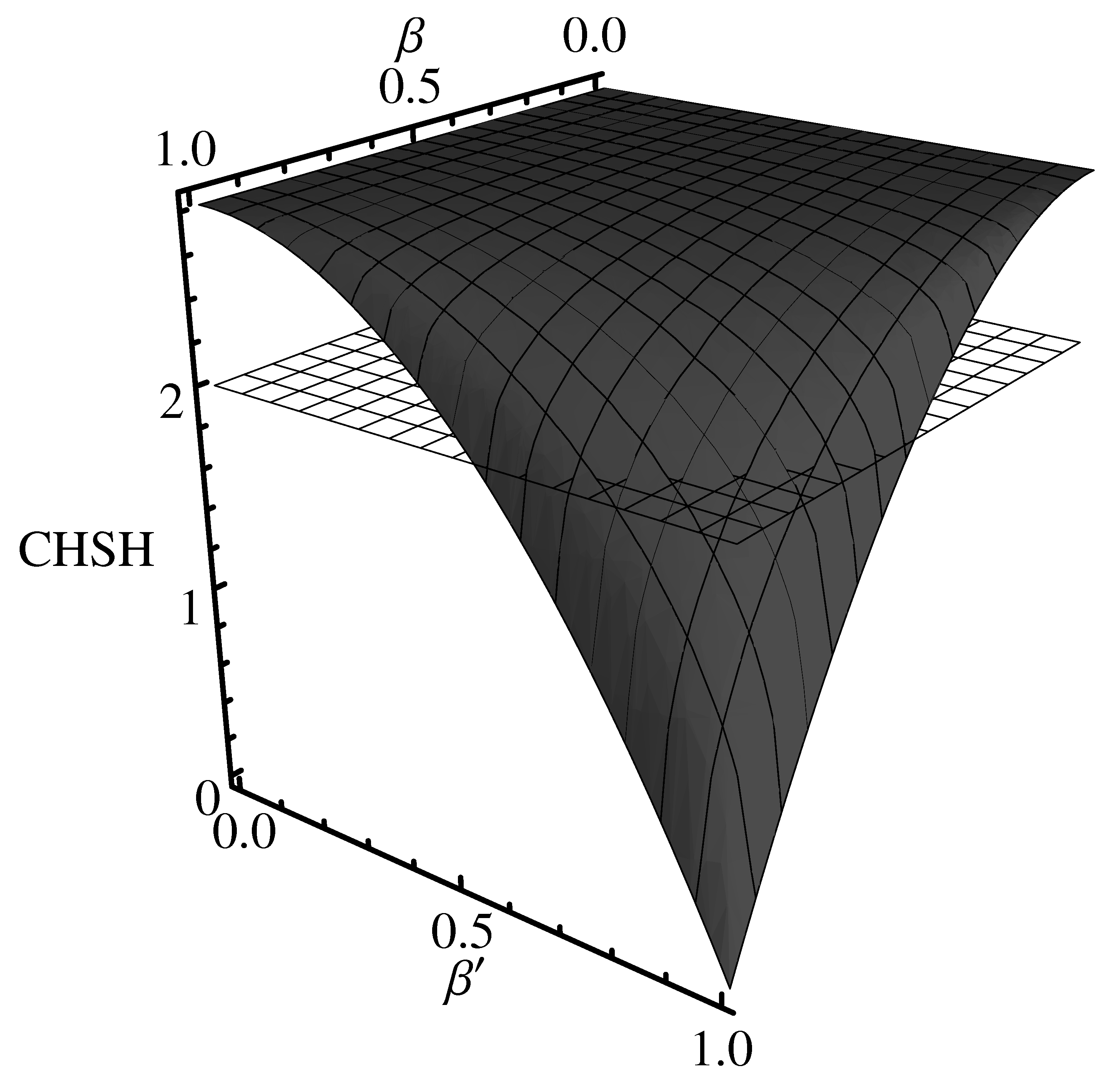
Figure 6: CHSH values versus velocity of the particles and the boosted frame, $\beta$ and $\beta^{\prime}$, respectively.

Now we are ready to test the locality condition by using CHSH inequality

$$CHSH=|C(\hat{a},\hat{b})+C(\hat{a^{\prime}},\hat{b})+C(\hat{a^{\prime}},\hat{b^{\prime}})-C(\hat{a},\hat{b^{\prime}})|\leq 2.$$ (161)

One can choose the measurement directions as the following

$$\hat{a} = (1/\sqrt{2},-1/\sqrt{2},0)$$

$$\hat{a^{\prime}} = (-1/\sqrt{2},-1/\sqrt{2},0)$$ (162)

$$\hat{b} = (0,1,0)$$

$$\hat{b^{\prime}} = (1,0,0)$$

corresponding to the case that they give maximum violation in the non relativistic limit. Then one obtains the result of the $CHSH$ as

$$CHSH=\sqrt{2}\bigg{(}1+\cos(2\theta_{W})\bigg{)}.$$ (163)

Using (95), this result can be defined in terms of the particle velocity $\beta$ and the velocity of the boosted frame $\beta^{\prime}$, as

$$CHSH=2\sqrt{2}\Bigg{(}\dfrac{\left(\sqrt{1-\beta^{2}}+\sqrt{1-\beta^{\prime 2}}\right)^{2}}{\left(\sqrt{1-\beta^{2}}+\sqrt{1-\beta^{\prime 2}}\right)^{2}+(\beta\beta^{\prime})^{2}}\Bigg{)}.$$ (164)

From these two equivalent results, it can be deduced that in the non relativistic domain, $\beta$ and $\beta^{\prime}\rightarrow 0$, as shown in the figure (6), we get the maximum violation as expected, however violation of the inequality starts before the ultra relativistic limit contrary to the claim in ahn , in which they use the spin operator defined in czachor . Also note that if the boost direction is parallel or anti-parallel to the direction of the particle as seen by the zero momentum frame, then there is no Wigner rotation, and we get the maximum violation as in caban1 .

V CONCLUSION

In this thesis, we have investigated the entanglement problem in the context of relativistic quantum mechanics. Entanglement lies at the heart of the quantum mechanics due to its non local character. In this sense, studying its properties in the framework of special relativity is crucial. For this purpose, we have first constructed the unitary irreducible representation of Poincaré group in the infinite dimensional Hilbert space. In this framework, the issue of finding the unitary irreducible representations of Poincaré group is reduced to that of the little group. Namely in this formalism Poincaré group reduces to the three dimensional rotation group for the massive cases, entangled states in different but equivalent frames undergo a Wigner rotation which changes its spin polarization direction.

On the other hand, since there are some ambiguities on the correct relativistic operator in the literature, we have critically studied physical requirements on it. Spin statistics must be a frame-independent property, and therefore square of the correct three-spin operator should be Lorentz invariant as implied by the second Casimir operator of Poincaré group.

Specifically, we have analyzed the Bell states under Lorentz transformations. Although these entangled states can mix, we have shown that the entanglement is a Lorentz invariant phenomena. This invariance has been shown for any entangled bipartite system by starting from the Schmidt decomposition. Then we have calculated the correlation function for the transformed states. Using the correlation, we have constructed the $CHSH$ inequality. At the first glance , $CHSH$ inequality seems to be satisfied for certain Wigner angles that depends on both the velocity of the particle and velocity of the boosted frame relative to the zero momentum frame of the entangled state. However, it is an illusion since changes in the velocities cause changes in the Wigner angle that can affect the superposition of the entangled states which violate the $CHSH$ inequality in different directions. Thus, it is natural that the initial dichotomous operators may satisfy the inequality for these entangled states. This confusing situation can be solved radically by performing the EPR experiment with the Wigner angle dependent dichotomous operators. As a result, Lorentz transformed entangled states still violates the Bell type inequalities in certain directions that may depend on the Wigner angle.

- (1) A. Einstein, B. Podolsky, and N. Rosen, Phys. Rev. 47, 777 (1935).
- (2) E. Schrödinger, Die gegenwärtige Situation in der Quantenmechanik, Naturwissenschaften 23, 807; 23 823; 23 844 (1935); English translation by J. D. Trimmer, The Present Situation in Quantum Mechanics: A Translation of Schrödinger’s “Cat Paradox” Paper, Proceedings of the American Philosophical Society 124, 323 (1980).
- (3) R. Horodecki, P. Horodecki, M. Horodecki, and K. Horodecki, Rev. Mod. Phys. 81, 2 (2009).
- (4) J. S. Bell, Physics 1, 195 (1964).
- (5) P. M. Alsing and G. J. Milburn, Lorentz Invariance of Entanglement, arXiv:quant-ph/0203051v1
- (6) M. Czachor, Phys. Rev. A 55, 72 (1997).
- (7) D. Ahn, H. J. Lee, Y. H. Moon, and S. W. Hwang, Phys. Rev. A 67, 012103 (2003).
- (8) P. Caban and J. Rembielin’ski, Phys. Rev. A 74, 042103 (2006).
- (9) P. Caban, J. Rembielin’ski and M. Wilczewski, Phys. Rev. A 79, 014102 (2009).
- (10) S. Moradi, Phys. Rev. A 77, 024101 (2008).
- (11) S. Weinberg, The Quantum Theory of Fields I, (Cambridge University Press, N.Y. 1995).
- (12) E. P. Wigner, Gruppentheorie und ihre Anwendung auf die Quantenmechanik der Atomspekten, (Braunschweig, 1931; English translation, Academic Press, Inc, New York, 1959).
- (13) W. I. Fushchich, A. G. Nikitin, Symmetries of Equations of Quantum Mechanics, (New York, 1994).
- (14) E.V. Stefanovich, Relativistic Quantum Dynamics, preprint arxiv:physics/0504062
- (15) J. Schwinger, Particles, Sources, and Fields, Vol. I (Addison-Wesley, Reading, Mass., 1970).
- (16) E. P. Wigner, Ann. Math. 40, 149 (1939).
- (17) D. Bohm and Y. Aharonov, Phys. Rev. 108, 1070 (1957).
- (18) A. Peres, Quantum Theory: Concepts and Methods (Kluwer, Dordrecht, 1993).
- (19) A. Aspect, P. Grangier, and G. Roger, Phys. Rev. Lett. 47, 460 (1981); A. Aspect, J. Dalibard, and G. Roger, Phys. Rev. Lett. 49, 1804 (1982); A. Aspect, P. Grangier, and G. Roger, Phys. Rev. Lett. 49, 91 (1982).
- (20) J. F. Clauser, M.A. Horne, A. Shimony and R. A. Holt, Phys. Rev. Lett. 23, 880-884 (1969).
- (21) B. S. Cirel’son, Lett. Math. Phys. 4, 93 (1980).