Ground-based CCD astrometry with wide field imagers

High precision astrometry requires an accurate geometric distortion solution. In this work, we present an average correction for the Blue Camera of the Large Binocular Telescope which enables a relative astrometric precision of $\sim$15 mas for the $B_{\rm Bessel}$ and $V_{\rm Bessel}$ broad-band filters. The result of this effort is used in two companion papers: the first to measure the absolute proper motion of the open cluster M 67 with respect to the background galaxies; the second to decontaminate the color-magnitude diagram of M 67 from field objects, enabling the study of the end of its white dwarf cooling sequence. Many other applications might find this distortion correction useful.

1 Introduction

Modern wide field imagers (WFI) equipped with CCD detectors began their operations at the end of the last century, however – after more than 10 years – their astrometric potential still remains somehow unexploited (see Anderson et al. anderson06 (2006), hereafter Paper I). It is particularly timely to begin exploring their full potential now that WFI start to appear also at the focus of the largest available 8m-class telescopes.

The present work goes in this direction, presenting a correction for the geometric distortion (GD) of the Blue prime-focus Large Binocular Camera (LBC), at the Large Binocular Telescope (LBT). Unlike in Paper I, in which we corrected the GD of the WFI at the focus of the 2.2m MPI/ESO telescope (WFI@2.2m) with a look-up table of corrections, for the LBC@LBT we will adopt the same technique described in Anderson & King (AK03 (2003), hereafter AK03), and successfully applied to the new Wide field Camera 3/UV-Optical channel on board the Hubble Space Telescope (Bellini & Bedin bb09 (2009), hereafter BB09).

This article is organized as follows: Section 2 briefly describes the telescope/camera set up; Section 3 presents the data set used. In section 4, we describe the steps which allowed us to obtain a solution of the GD, for each detector separately, while in Section 5 we presents a (less accurate) inter-chip solution. Distortion stability is analyzed in Section 6, and a final Section summarizes our results.

Figure 1: (Left): LBC-Blue mosaic layout; “$\ast$” marks the center for each chip (see Sect. 3 for the operative definition of centers and chips), while “+” marks the here defined center of the mosaic. (Right): Each MEF file consists of 4 images. Each image is composed by one scientific region and two overscan regions, covering the first 50 and the last 206 pixel columns (shaded).

2 The Large Binocular Camera Blue

The LBT is a large optical/infrared telescope that utilizes two mirrors, each having a diameter of 8.4 meters. The focal ratio of the LBT primary mirrors ($F$/1.14) and its large diameter are factors that require a careful development of the corrector for a prime-focus camera. The blue channel of the LBC (LBC-Blue) is mounted at the prime focus of the first LBT unit. The corrector, consisting of three lenses, is designed to correct spherical aberration, coma, and field curvature, according to the design by Wynne (wynne96 (1996)). The last two of these three lenses are sub-divided in two elements each, with the last one being the window of the cryostat (Ragazzoni et al. ragazzoni00 (2000), ragazzoni06 (2006); Giallongo et al. giallongo08 (2008)). The final LBC-Blue focal-ratio is $F$/1.46.

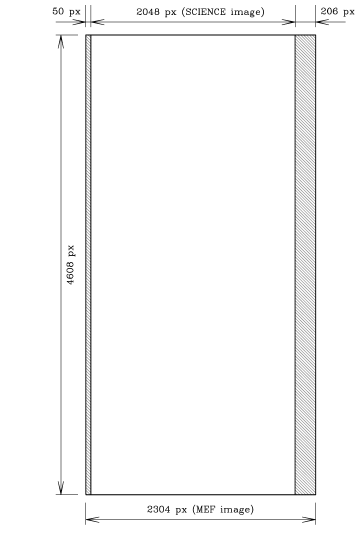
The LBC-Blue employs an array of four 16-bit e2v 42-90 (2048$\times$4608) chips, with a reference pixel-scale of $0\aas@@fstack{\prime\prime}2297\,{\rm pix}^{-1}$ (this work), providing a total Field of View (FoV) of $\sim$$24^{\prime}$$\times$$25^{\prime}$. The four chips are mounted on the focal plane in such a way as to maximize the symmetry of the field, with three chips contiguous longside, and the fourth one rotated 90 degrees anti-clockwise, and centered above the others. The LBC-Blue layout is shown on the left hand of Fig. 1. Row estimates of the intra-chip gaps are expressed as the nearest integer pixel. Numbers between square brackets are chip identification numbers, as read from the raw Multi Extension Fits (MEF) file. Average rotation angles are given with respect to chip # 2, chosen as reference (we will see in Section 5 how to bring positions from each chip into a common corrected meta-chip system). On the right hand of Fig. 1 we show, in units of raw pixel coordinates, the dimensions of each chip, which consists of the scientific image in between two overscan regions (shaded areas Fig. 1, which cover the first 50 and the last 206 pixel columns).

During the optical design phase, GD (of pin-cushion type) was not considered as an aberration, since it may be corrected at post-processing stages. The GD is found to be always below the 1.75% level (Giallongo et al. giallongo08 (2008)). This is translated in offsets as large as 50 pixels ($\sim$11 arcsec) from corner to corner of the LBC-Blue FoV. Obviously, the correction of such a large GD is of fundamental importance for high precision astrometric measurements. Note that in the following, with the term “geometric distortion” we are lumping together several effects: the optical field-angle distortion introduced by camera optics, light-path deviations caused by the filters (in this case $B_{\rm Bessel}$ and $V_{\rm Bessel}$), non-flat CCDs, alignment errors of CCDs on the focal plane, etc.

Table 1: Log of M 67 data used in this work.

Date	Filter	#Images$\times$Exp. time	Airmass	Image Quality
		(s)	$(\sec z)$	(arcsec)
Feb 22, 2007	$V_{\rm Bessel}$	$\!\!\!1\times 15$,$1\times 330$,$17\times 110\!\!\!$	1.07-1.13	0.62-1.31
Feb 27, 2007	$V_{\rm Bessel}$	$25\times 100$	1.07-1.10	0.84-1.26
Mar 16, 2007	$B_{\rm Bessel}$	$25\times 180$	1.07-1.14	0.84-1.08

Figure 2: (Left): Dither pattern, in pixel units, of the $V$ images used to solve for the geometric distortion. We used both small and large dithers to adequately sample the GD. Red crosses mark the center of LBC-Blue mosaic, (1025, 3355) position in the coordinate system of chip # [2], as defined in Fig. 1). The original pattern was designed to be a rhomboidal array of 5$\times$5 pointings (see text). Unfortunately some of the images with the small dither pattern were not usable. (Right): Depth-of-coverage map for the same images.

Raw data images are contained in a single MEF file with four extensions, one for each chip, constituted by 2304$\times$4608 pixels, containing overscan regions. The scientific area of these chips is located within pixel (51, 1) and pixel (2098, 4608) (i.e. 2K$\times$4.5K pixels, see right panel of Fig. 1). For reasons of convenience, we added an extra pixel (flagged at a value of $-$475) to define the borders of the 2048$\times$4608 pixel scientific regions, and we will deal exclusively with 2050$\times$4610 arrays (work-images). Again for reasons of convenience, since chip # [4] is stored along the same physical dimensions as the other three in the raw MEF file, we decided to rotate it by 90 degrees anti-clockwise.

Hereafter, when referring to $x$ and $y$ positions, we will refer to the raw pixel coordinates measured on these work-images, and – unless otherwise specified – we will refer to the work-image of the chip # [$k$], simply as [$k$]. Transformation equations to convert from the raw pixel coordinates of the archive MEF file $(x^{\rm MEF}_{k},y^{\rm MEF}_{k})$ to the pixel coordinates of the work-images $(x,y)$ are as follows:

$$k=1,2,3:\leavevmode\nobreak\ \left\{\begin{array}[]{rcl}\displaystyle x&\!\!\!=\!\!\!&x^{\rm MEF}_{k}-49\\ \displaystyle y&\!\!\!=\!\!\!&y^{\rm MEF}_{k}+1\\ \end{array}\right.\\$$

$$\leavevmode\nobreak\ k=4:\leavevmode\nobreak\ \left\{\begin{array}[]{rcl}\displaystyle x&\!\!\!=\!\!\!&4610-y^{\rm MEF}_{k}\\ \displaystyle y&\!\!\!=\!\!\!&x^{\rm MEF}_{k}-49.\\ \end{array}\right.$$

[For clarity, every LBC-Blue image is a MEF file, from which we define 4 work-images. Moreover, we will treat every chip of each image independently.]

3 The data-set

During LBT science-demonstration time, between February and March 2007, we obtained (under the Italian guaranteed time) about four hours to observe the old, metal-rich open cluster M 67 ($\alpha=08^{\rm h}51^{\rm m}23^{\rm s}.3$, $\delta=+11^{\circ}49\arcmin 02\arcsec$, J2000.0, Yadav et al. yadav08 (2008), hereafter Paper II). The aim of the project is to reach the end of the DA white dwarf (WD) cooling sequence (CS) in the two filters $V_{\rm Bessel}$ and $B_{\rm Bessel}$ (hereafter simply $V$ and $B$). In addition, we want to compute proper motions for a sample of objects in the field by combining these LBC@LBT exposures with archival images collected 10 years before at the Canada France Hawaii Telescope (CFHT). The pure sample of WD members will serve to better understand the physical processes that rule the WD cooling in metal-rich clusters. A necessary first step to get accurate proper motions is to solve the GD for the LBC-Blue. The results of the investigation on the WD CS of M 67, and its absolute proper motion, are presented in two companion papers (Bellini et al. 2010a , 2010b ); here we will focus on the GD of LBC-Blue, providing a solution that might be useful to a broader community of LBC-Blue users.

The observing strategy had to arrange both the scientific goals of the project and the need to solve for the geometric distortion. As an educated guess, the adopted procedure to solve for the geometric distortion is the auto-calibration described in great detail in Paper I, which still represents the state of the art in ground-based CCD astrometry with wide-field imagers.

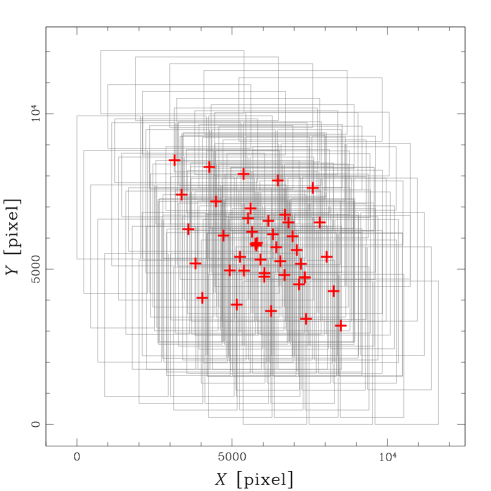
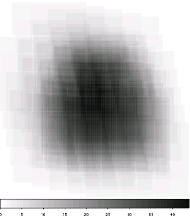
With the idea to map the same patch of the sky in different locations on the same chip, as well as on different chips, we chose a particular pointing set up, constituted by an array of 5$\times$5 observations, dithered in such a way that a star never falls two times on the same gap between the chips. All 25 exposures of a given dither sequence were executed consecutively. The 5$\times$5 dither pattern is repeated adopting small ($\sim$100$\arcsec$) and large ($\sim$200$\arcsec$) steps in filter $V$, and only small steps in the $B$ filter. Figure 2 shows the dither pattern and the depth-of-coverage map for all our $V$ exposures. Table 1 gives the log of observations for both $B$ and $V$ exposures. All the images were collected in service mode.

Unfortunately, not all the exposures met the desired specifications of our proposal (dark-night conditions and seeing better than $0\aas@@fstack{\prime\prime}8$). In particular, all the $V$ images with large dithers are affected by anomalously high background values (up to $\sim$20 000 counts for a 100 s exposure, thus limiting us at the faint magnitudes). Moreover, 6 out of the 25 $V$ images taken with small dithers have an image quality well above $1\aas@@fstack{\prime\prime}5$ (probably related to guide-star system problems). These images are of no use for our purpose, and were not considered in the present study.

Our GD solution will be first obtained for the $V$ filter images, and later tested, and eventually re-derived, for the $B$ filter ones. To measure star positions and fluxes, we developed a reduction method that is mostly based on the software img2xym_WFI (Paper I). This new software (img2xym_LBC) similarly generates a list of positions, fluxes, and a quality of the PSF-fit values (see Anderson et al. anderson08 (2008)) for each of the measured objects in each of the four chips. Details of the PSF-fitting software img2xym_LBC and the final M 67 astro-photometric catalog will be presented in a subsequent paper of this series (which will also deal with photometric zero point variations and PSF variability).

4 Auto-calibration

The most straightforward way to solve for the GD would be to observe a field where there is a prior knowledge of the positions of all the stars in a distortion-free reference frame. [A distortion-free reference frame is a system that can be transformed into any another distortion-free frame by means of conformal transformations.] GD would then show itself immediately as the residuals between the observed relative positions of stars and the ones predicted by the distortion-free frame (on the basis of a conformal transformation). Unfortunately, such an “astrometric flat-field” with the right magnitude interval, source density, and accuracy, is difficult to find and astronomers are often left with the only option of auto-calibration.

The basic principle of auto-calibration is to observe the same stars in as many different locations on the detector as possible, and to compute their average positions once they are transformed onto a common reference frame. Ideally, a star should be observed from corner to corner in the FoV. This means that the total dither has to be as large as the FoV itself (see Fig. 2).

If the observations are taken with a symmetric dither pattern, the systematic errors will have a random amplitude, and the stars’ averaged position will provide a better approximation of their true position in a distortion-free frame (the master frame). This master frame – as defined by the averaged position of the sources in the FoV – will then serve as a first guess for the construction of an astrometric flat-field, which in turn can be used (as we will see in detail below) to compute star-position residuals (hereafter simply residuals), necessary to obtain a first estimate of the GD for each chip. Single chips are then individually corrected with these preliminary GD solutions (one for each chip) and the procedure of deriving the master frame is repeated. With the new-derived master frame, new (generally smaller) residuals are computed, and the procedure is iteratively repeated until convergence is reached (see below).

The overall distortion of LBC-Blue is large enough ($\sim$50 pixels) that – to facilitate the cross-correlation of positions of objects observed in different locations on the detector – it becomes very convenient to perform a preliminary (although crude) correction.

As a first guess for the master frame, we used the best astrometric flat-field available in the literature for the M 67 field: the astro-photometric catalog recently published in Paper II. This catalog was obtained with images taken with the WFI@2.2m; it is deeper with respect to other wide-field catalogs (i.e., UCAC2, USNO-A2, and 2MASS), has $V$ photometry, and its global astrometric accuracy is of the order of $\sim$50 mas. Nevertheless, this catalog is far from ideal; even the faintest – poorly measured – stars of Paper II are close to saturation in our LBC-Blue images, and the total number of usable (even if saturated) objects was never above $\sim$250 per chip (among which less than $\sim$40 per chip were unsaturated). We also chose to re-scale the pixel coordinates of the Paper II catalog (with an assumed WFI@2.2m pixel-scale of 238 mas, Paper I) to the average pixel-scale of LBC-Blue, adopting for it the median value of $225.4$ mas/pixel (as derived by Giallongo et al. giallongo08 (2008)). Since the scale is a free parameter in deriving GD correction, choosing a particular scale value will not invalidate the solution itself. Later we will derive the average scale of [2] in its central pixel (1025,2305), and we will determine the absolute value of our master-frame plate scale by comparison with objects in the Digital Sky Survey, and study the average inter-chip scale variations with time and conditions.

Once this first-guess solution is obtained, it is easier to cross-correlate the star catalogs from each LBC-Blue work-image with respect to a common reference frame, in order to perform the auto-calibration procedure, as described in detail in the following subsections.

4.1 Deriving a self-consistent solution

We closely followed the auto-calibration procedures described in detail – and used with success – in AK03 to derive the GD correction for each of the four detectors of WFPC2. The auto-calibration method consists of two steps: 1) deriving the master frame, and 2) solving for the GD for each chip, individually. These two steps are then repeated interactively, until both the geometric distortion solutions and the positions in the master-list converge.

Figure 3: The master star-list map.

4.1.1 The master-list

As aforementioned, only during the very first iteration did we use the Paper II catalog as a master frame to get the preliminary best guess of the GD for each chip. In all the subsequent iterations, the master frame was obtained from all the available LBC work-images (i. e., the master-list is made with images taken within few days). Conformal transformations are used to bring star positions, as measured in each work-image, into the reference system of the current master frame. We used only well-measured, unsaturated objects with a stellar profile. The final master-list contains 2374 uniformly spread stars (see Fig. 3), with coordinates $(X^{\rm master},Y^{\rm master})_{i}$, with $i=1,\dots,2374$, that were observed, at each iteration, in at least 3 different images. As we can see on the right panel of Fig. 2, stars falling in the center of our FoV can be observed up to 44 times in the $V$-filter, i. e. the maximum overlap among the $V$ exposures. We have at most 25 observations for a given star in the case of the $B$-filter exposures.

4.1.2 Modeling the geometric distortion

As in AK03 and in BB09, we represent our solution with two third-order polynomials. Indeed, we found that with two third-order polynomials our final GD correction has a precision level of $\sim$0.04 pixel in each coordinate ($\sim$10 mas), and higher orders were unnecessary, with this precision level (as we will see) being well within the instrument stability. We performed tests with fourth- and fifth-order polynomials, obtaining comparable results in term of GD-solution accuracy, but at the expense of using a large number of degrees of freedom in modeling the GD solution.

Having an independent solution for each chip, rather than one that uses a common center of the distortion for the whole FoV, allows a better handle on individual detector effects, such as a different relative tilt of the chip surfaces, etc. We chose a pixel close to the physical center of each chip as reference position, with respect to solve for the GD, regardless of its relative position with respect to the principal axes of the optical system. The adopted centers of our solution are the locations $(x_{\circ},y_{\circ})_{k=1,2,3}=(1025,2305)$ for chips [1], [2], [3], and the $(x_{\circ},y_{\circ})_{4}=(2305,1025)$ for chip [4], all in the raw pixel coordinates of the work-images.

For each $i$-star in each $k$-chip of each $j$-MEF file, the distortion corrected position $(x_{i,j,k}^{\rm corr},y_{i,j,k}^{\rm corr})$ is the observed position plus the distortion correction $(\delta x_{i,j,k},\delta y_{i,j,k})$:

$$\left\{\begin{array}[]{c}\displaystyle x_{i,j,k}^{\rm corr}=x_{i,j,k}+\delta x_{i,j,k}(\tilde{x}_{i,j,k},\tilde{y}_{i,j,k})\\ \displaystyle y_{i,j,k}^{\rm corr}=y_{i,j,k}+\delta y_{i,j,k}(\tilde{x}_{i,j,k},\tilde{y}_{i,j,k}),\\ \end{array}\right.$$

where $\tilde{x}_{i,j,k}$ and $\tilde{y}_{i,j,k}$ are the normalized positions, defined as:

$$\left\{\begin{array}[]{c}\displaystyle\tilde{x}_{i,j,k}=\frac{x_{i,j,k}-(x_{\circ})_{k}}{(x_{\circ})_{k}}\\ \displaystyle\tilde{y}_{i,j,k}=\frac{y_{i,j,k}-(y_{\circ})_{k}}{(y_{\circ})_{k}}.\\ \end{array}\right.$$

[Normalized positions make it easier to recognize the magnitude of the contribution given by each solution term, and their numerical round-off.]

Figure 4: Residual trends for the four chips when we use uncorrected star positions. The size of the residual vectors is magnified by a factor of 25. For each chip, we also plot the single residual trends along the $x$ and $y$ axes. Units are expressed as LBC-Blue raw pixels.

Figure 5: Same as Fig. 4, but for our corrected star positions. The size of the residual vectors is now magnified by a factor of 500.

The final distortion correction, for each star in each work-image, is given by the following two third-order polynomials (we omitted here $i,j,k$ indexes for simplicity):

$$\left\{\begin{array}[]{rcl}\displaystyle\delta x&\!\!\!=\!\!\!&a_{1}\tilde{x}+a_{2}\tilde{y}+a_{3}\tilde{x}^{2}+a_{4}\tilde{x}\tilde{y}+a_{5}\tilde{y}^{2}+a_{6}\tilde{x}^{3}+a_{7}\tilde{x}^{2}\tilde{y}\\ &&\phantom{a_{1}\tilde{x}}+a_{8}\tilde{x}\tilde{y}^{2}+a_{9}\tilde{y}^{3}\\ \displaystyle\delta y&\!\!\!=\!\!\!&b_{1}\tilde{x}+b_{2}\tilde{y}+b_{3}\tilde{x}^{2}+b_{4}\tilde{x}\tilde{y}+b_{5}\tilde{y}^{2}+b_{6}\tilde{x}^{3}+b_{7}\tilde{x}^{2}\tilde{y}\\ &&\phantom{a_{1}\tilde{x}}+b_{8}\tilde{x}\tilde{y}^{2}+b_{9}\tilde{y}^{3}.\\ \end{array}\right.$$

Our GD solution is thus fully characterized by 18 coefficients: $a_{1},\dots,a_{9}$, $b_{1},\dots,b_{9}$. As done in AK03 and BB09, we imposed $a_{1,k}=0$ and $a_{2,k}=0$ to constrain the solution so that, at the center of the chip, it will have its $x$-scale equal to the one at the location $(x_{\circ},y_{\circ})$, and the corrected axis $y_{\rm corr}$ aligned with its $y$-axis at the same location. On the other hand, $b_{1,k}$ and $b_{2,k}$ must be free to assume whatever values fit best, to account for differences in scale and perpendicularity of detector’s axes. Therefore, we only have to compute 16 coefficients (for each chip) to derive our GD solution.

4.1.3 Building the Residuals

Each $i$-star in the master frame is conformally transformed into each $k$-work-image/$j$-file, and cross-identified with the closest source. We indicate such transformed positions with $(X_{i}^{\rm master})^{T_{j,k}}$ and $(Y_{i}^{\rm master})^{T_{j,k}}$. Each of such cross-identifications, when available, generates a pair of positional residuals:

$$\left\{\begin{array}[]{rcl}\displaystyle\Delta x_{i,j,k}&\!\!\!=\!\!\!&x_{i,j,k}^{\rm corr}-(X_{i}^{\rm master})^{T_{j,k}}\\ \displaystyle\Delta y_{i,j,k}&\!\!\!=\!\!\!&y_{i,j,k}^{\rm corr}-(Y_{i}^{\rm master})^{T_{j,k}},\\ \end{array}\right.$$

which reflect the residuals in the GD (with the opposite sign), and depend on where the $i$-star fell on the $k$/$j$ work-image/file (plus random deviations due to non-perfect PSF-fitting, photon noise, and errors in the transformations). [Note that, at the first iteration, $(x^{\rm corr},y^{\rm corr})_{i,j,k}$$=$$(x,y)_{i,j,k}$.] In each chip we have typically 120-130 high-signal stars in common with the master frame, leading to a total of $\sim$5500 residual pairs per chip.

These residuals were then collected into a look-up table made up of 11$\times$25 elements, each related to a region of 186.4$\times$184.4 pixels (25$\times$11 elements of 184.4$\times$186.4 for chip [4]). We chose this particular grid setup because it offers the best compromise between the need of an adequate number of grid points to model the GD (the larger, the better) and an adequate sampling of each grid element (we required to have at least 10 pairs of residuals in each grid element). For each grid element, we computed a set of five 3$\sigma$-clipped quantities: $\overline{x}_{m,n,k}$, $\overline{y}_{m,n,k}$, $\overline{\Delta x}_{m,n,k}$, $\overline{\Delta y}_{m,n,k}$, and $P_{m,n,k}$; where $\overline{x}_{m,n,k}$ and $\overline{y}_{m,n,k}$ are the average positions of all the stars within the grid element $(m,n)$ of the $k$-chip, $\overline{\Delta x}_{m,n,k}$ and $\overline{\Delta y}_{m,n,k}$ are the average residuals, and $P_{m,n,k}$ is the number of stars that were used to calculate the previous quantities. These $P_{m,n,k}$ will also serve in associating a weight to the grid cells when we fit the polynomial coefficients.

4.1.4 Iterations

To obtain the 16 coefficients describing the two polynomials ($a_{q,k}$ with $q=3,\dots,9$, and $b_{q,k}$ with $q=1,\dots,9$) that represent our GD solution in each chip, we perform a linear least square fit of the $N$=$m$$\times$$n$=$11$$\times$25$=$275 cells (hereafter we will use the notation $p$$=$$1,\dots,N$, instead of the two $m$$=$$1,\dots,11$ and $n$$=$$1,\dots,25$). In the linear least square fit, we can safely consider the errors on the average positions $\overline{x}_{p,k}$, $\overline{y}_{p,k}$ (i.e., $\overline{x}_{m,n,k}$, $\overline{y}_{m,n,k}$) negligible with respect to the uncertainties on the average residuals $\overline{\Delta x}_{p,k}$, $\overline{\Delta y}_{p,k}$ (i.e., $\overline{\Delta x}_{m,n,k}$, $\overline{\Delta y}_{m,n,k}$). Thus, for each chip, we can compute the average distortion correction in each cell $(\overline{\delta x}_{p,k}$, $\overline{\delta y}_{p,k})$ with $N$ relations of the form:

$$k=1,\dots,4;\leavevmode\nobreak\ p=1,\dots,N:\leavevmode\nobreak\ \left\{\begin{array}[]{c}\overline{\delta x}_{p,k}=\displaystyle\sum_{q=3}^{9}a_{q,k}t_{q,p,k}\\ \overline{\delta y}_{p,k}=\displaystyle\sum_{q=1}^{9}b_{q,k}t_{q,p,k}\\ \end{array}\right.$$

(where $t_{1,p,k}=\overline{\tilde{x}}_{p,k}$, $t_{2,p,k}=\overline{\tilde{y}}_{p,k}$, …, $t_{9,p,k}={{\overline{\tilde{y}}}}^{3}_{p,k}$), concerning the 16 unknown quantities – or fitting parameters – $a_{q,k}$ and $b_{q,k}$, for each chip.

In order to solve for $a_{q,k}$ and $b_{q,k}$, we defined, for each chip, one 9$\times$9 matrix $\mathcal{M}_{k}$ and two 9$\times$1 column vectors ${\mathcal{V}}_{a,k}$ and ${\mathcal{V}}_{b,k}$:

$$\!\mathcal{M}_{k}\!=\!\displaystyle\left(\begin{array}[]{cccc}\sum_{p}P_{p,k}t_{1,p,k}^{2}&\sum_{p}P_{p,k}t_{1,p,k}t_{2,p,k}\!&\cdots&\!\!\sum_{p}P_{p,k}t_{1,p,k}t_{9,p,k}\!\!\\ \!\!\sum_{p}P_{p,k}t_{2,p,k}t_{1,p,k}\!\!&\!\!\sum_{p}P_{p,k}t_{2,p,k}^{2}\!\!&\!\!\cdots\!\!&\!\!\sum_{p}P_{p,k}t_{2,p,k}t_{9,p,k}\!\!\\ \!\vdots&\!\!\vdots&\!\!\ddots&\!\!\vdots\\ \!\!\sum_{p}P_{p,k}t_{9,p,k}t_{1,p,k}\!\!&\!\!\sum_{p}P_{p,k}t_{9,p,k}t_{2,p,k}\!&\cdots&\sum_{p}P_{p,k}t_{9,p,k}^{2}\\ \end{array}\right);$$

$$\mathcal{V}_{a,k}=\left(\begin{array}[]{c}\sum_{p}P_{p,k}t_{1,p,k}\overline{\Delta x}_{p,k}\\ \sum_{p}P_{p,k}t_{2,p,k}\overline{\Delta x}_{p,k}\\ \vdots\\ \sum_{p}P_{p,k}t_{9,p,k}\overline{\Delta x}_{p,k}\\ \end{array}\right);\,\,\,\,\,\mathcal{V}_{b,k}=\left(\begin{array}[]{c}\sum_{p}P_{p,k}t_{1,p,k}\overline{\Delta y}_{p,k}\\ \sum_{p}P_{p,k}t_{2,p,k}\overline{\Delta y}_{p,k}\\ \vdots\\ \sum_{p}P_{p,k}t_{9,p,k}\overline{\Delta y}_{p,k}\\ \end{array}\right).$$

Table 2: Coefficients of the third-order polynomial in each chip used to represent our geometric distortion in the final solution for the $V$ filter.

Term $\!(q)\!\!\!\!\!$	Polyn.	$a_{q,[1]}$	$b_{q,[1]}$	$a_{q,[2]}$	$b_{q,[2]}$	$a_{q,[3]}$	$b_{q,[3]}$	$a_{q,[4]}$	$b_{q,[4]}$
1	$\tilde{x}$	$+0.0000\!$	$\!+6.3877\!$	$\!+0.0000\!$	$\!+0.1638\!$	$\!+0.0000\!$	$\!-6.2855\!$	$\!+0.0000\!$	$\!+1.0239$
2	$\tilde{y}$	$+0.0000\!$	$\!+20.2053\!$	$\!+0.0000\!$	$\!-2.7878\!$	$\!+0.0000\!$	$\!+20.2021\!$	$\!+0.0000\!$	$\!-16.5767$
3	$\tilde{x}^{2}$	$-7.1942\!$	$\!+0.6063\!$	$\!-0.1033\!$	$\!+0.6919\!$	$\!+7.2181\!$	$\!+0.6900\!$	$\!+0.9713\!$	$\!-15.7873$
4	$\tilde{x}\tilde{y}$	$+3.2801\!$	$\!-10.7004\!$	$\!+3.6108\!$	$\!-0.2218\!$	$\!+3.5260\!$	$\!+10.5439\!$	$\!-13.8197\!$	$\!+0.3543$
5	$\tilde{y}^{2}$	$-12.2026\!$	$\!+11.3321\!$	$\!-0.3165\!$	$\!+11.7370\!$	$\!+12.1294\!$	$\!+11.7808\!$	$\!+0.0850\!$	$\!-9.0966$
6	$\tilde{x}^{3}$	$-1.1416\!$	$\!-0.0136\!$	$\!-1.1606\!$	$\!+0.0168\!$	$\!-1.0659\!$	$\!+0.0204\!$	$\!-13.1945\!$	$\!+0.0213$
7	$\tilde{x}^{2}\tilde{y}$	$-0.1559\!$	$\!-2.5312\!$	$\!-0.0204\!$	$\!-2.5133\!$	$\!+0.1460\!$	$\!-2.6083\!$	$\!+0.1596\!$	$\!-5.4927$
8	$\tilde{x}\tilde{y}^{2}$	$-5.7174\!$	$\!-0.3752\!$	$\!-5.7339\!$	$\!-0.1705\!$	$\!-5.8841\!$	$\!+0.2810\!$	$\!-2.3973\!$	$\!+0.0324$
9	$\tilde{y}^{3}$	$-0.2740\!$	$\!-12.6714\!$	$\!+0.0087\!$	$\!-12.4949\!$	$\!+0.1189\!$	$\!-13.1913\!$	$\!+0.0876\!$	$\!-0.9556$

The solution is given by two 9$\times$1 column vectors $\mathcal{A}_{k}$ and $\mathcal{B}_{k}$, containing the best fitting values for $a_{q,k}$ and $b_{q,k}$, obtained as:

$${\mathcal{A}_{k}}=\left(\begin{array}[]{c}a_{1,k}\\ a_{2,k}\\ \vdots\\ a_{9,k}\\ \end{array}\right)={\mathcal{M}_{k}}^{-1}{\mathcal{V}}_{a,k};\,\,\,\,\,\,\,\,\,\,\,\,\,\,\,{\mathcal{B}_{k}}=\left(\begin{array}[]{c}b_{1,k}\\ b_{2,k}\\ \vdots\\ b_{9,k}\\ \end{array}\right)={\mathcal{M}_{k}}^{-1}{\mathcal{V}}_{b,k}.$$

With the first set of calculated coefficients $a_{q,k}$ and $b_{q,k}$ we computed the corrections $\delta x_{i,j,k}$ and $\delta y_{i,j,k}$ to be applied to each $i$-star of the $k$-chip in each $j$-MEF file, but actually we corrected the positions only by half of the recommended values, to guarantee convergence. With the new improved star positions, we start-over and recalculated new residuals. The procedure is iterated until the difference in the average corrections from one iteration to the following one – for each grid point – became smaller than 0.001 pixels. Convergence was typically reached after $\sim$20–30 iterations.

4.2 The GD solution

Once new corrected star positions have been obtained for all the images, we can derive a new master frame, and consequently improve our GD solution for each chip, simply by repeating the procedure used to determine the polynomial coefficients. At the end of each iteration, star positions in the newly derived master frame are closer than before to the ones of a distortion-free frame, and provide a better reference on which to calculate the GD correction. After 15 such iterations, we were able to reduce star-position residuals from the initial average of $\sim$4 pixels down to 0.085 pixels ($\sim$20 mas) (or $\sim$15 mas for each single coordinate). [A further iteration proved to give no significant improvements to our solution.]

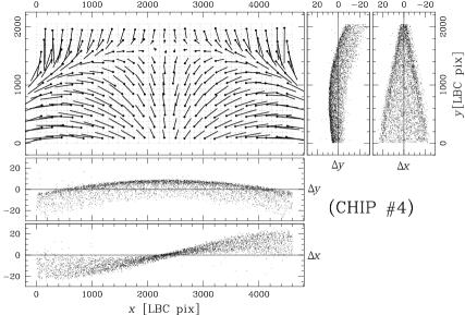
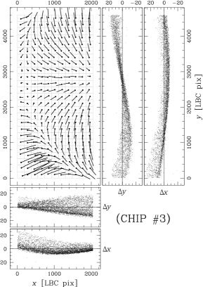
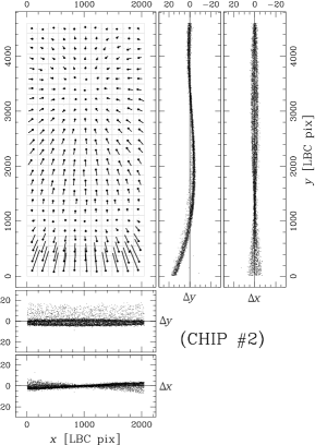
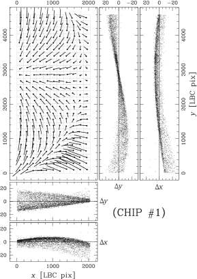
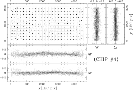
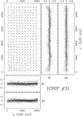
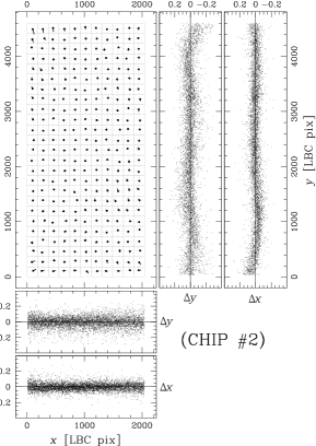
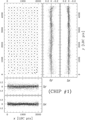
In Fig. 4 we show – for each chip – the residual of uncorrected star positions versus the predicted positions of our final master frame, which is representative of our GD solution. For each chip, we plot the 11$\times$25 cells used to model the GD, each with its distortion vector magnified by a factor of 25. Residual vectors go from the average position of the stars belonging to each grid cell $(\overline{x},\overline{y})$ to the corrected one. We also show the overall trend of residuals $\Delta x$, $\Delta y$ along $x$ and $y$ directions. Note the symmetric shape of the geometric distortion around the center of the FoV. In Fig. 5 we show, in the same way, the remaining residuals after our GD solution is applied. This time we magnified the distortion vectors by a factor of 500. [Note that, close to chip edges, remaining residuals are larger that the average. We suggest to exclude those regions for high precision astrometry.] The coefficients of the final solution for the four chips are given in Table 2.

Figure 6: (Top): Positional r.m.s. as a function of the instrumental $V$ magnitude without GD correction. (Middle): Same plot, but with GD correction. Corrected catalogs are transformed into the reference frame using a conformal transformation. (Bottom): Same plot, but using the most general linear transformations (6 parameters) to bring the corrected catalogs into the reference frame, instead of a conformal transformation (4 parameters). Vertical dashed lines mark the magnitude interval used to calculate median values for the positional r.m.s.

4.3 Accuracy of the GD Solution

The best estimate of the true errors in our GD solution is given by the size of the r.m.s. of the position residuals observed in each work-image, which have been GD-corrected, and transformed into the reference frame $(X_{i,j,k},Y_{i,j,k})$. Since each star has been observed in several work-images and in different regions of the detectors, the consistency of these star positions, once transformed in the coordinate system of the distortion-free reference frame $(X_{i}^{\rm master},Y_{i}^{\rm master})$, immediately quantifies how well we are able to put each image into a distortion-free system.

Figure 7: (From Top to Bottom): Positional r.m.s. as function of the instrumental $B$ magnitude when no GD correction is applied at all. (Next): Same plot, but after the $V$-derived GD correction applied, and using conformal transformations to transform corrected catalogs into the reference frame. (Next): Same plot, but using the most general linear transformations (6 parameters). (Next): Positional r.m.s. after the GD correction obtained from $B$ images is applied, and using conformal transformations. (Bottom): Same as above but using a general linear transformations. Vertical dashed lines mark the magnitude interval used to calculate median values for the positional r.m.s.

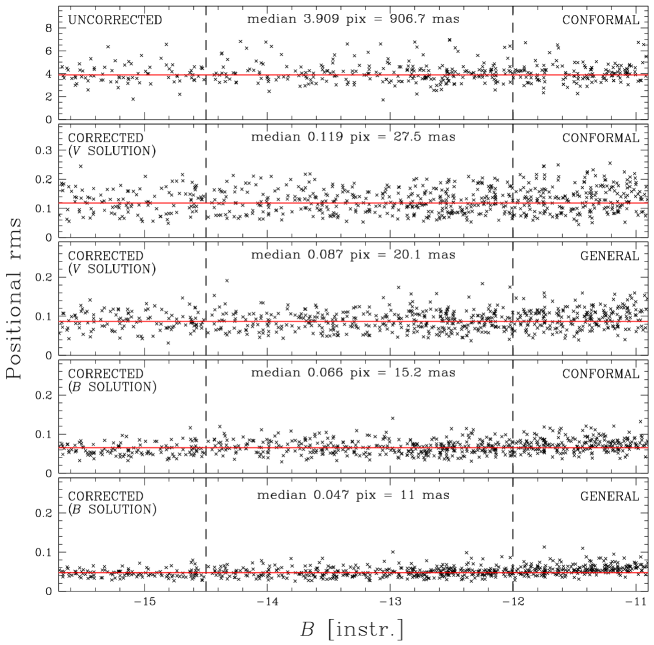
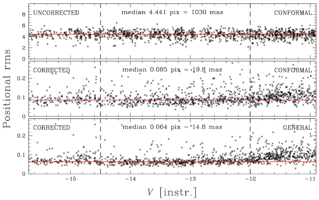
In the top panel of Fig. 6 we show the size of these r.m.s. versus the instrumental $V$ magnitude, before GD correction is applied – at all – to the observed positions, before transforming them into the master-frame using a conformal transformation. The instrumental magnitude ($m_{\rm instr.}$) has been computed as the sum of the pixel’s digital numbers (DNs) under the best fitted PSF (i.e. $m_{\rm instr.}$$=$$-2.5\log{[\Sigma({\rm DNs}})]$). For reference, in images with a seeing of $0\aas@@fstack{\prime\prime}6$, saturation begins at $m_{\rm instr.}$$=$$-$14.1, while if the seeing is $\sim$$1\aas@@fstack{\prime\prime}0$, the saturation level can reach $m_{\rm instr.}$$=$$-$15.2. (This simply means that in these two cases, the brightest pixels contain $\sim$12% or $\sim$4% of the flux, respectively, enabling to collect more or fewer photons before saturation is reached in the brightest pixel.)

The r.m.s. are computed from the values $\sqrt{[(X_{i}^{\rm master})^{T_{j,k}}-X_{i}^{\rm master}]^{2}+[(Y_{i}^{\rm master})^{T_{j,k}}-Y_{i}^{\rm master}]^{2}}$. Only stars in the master-list observed in at least 9 images, and within $\sim$2.5 magnitudes below the saturation level (between the dashed lines) were considered to test the accuracy of the GD solution, because faint stars are dominated by random errors. Note, however, that we applied our GD solution to all the sources in our catalogs. We can see that if no GD correction is applied, the positional r.m.s. exceed 4.4 pixels (i.e. a whole arcsec). In some locations on the chips individual displacements can exceed 20 pixels (5 arcsec), see Fig. 4.

Middle panel of Fig. 6 shows that, once our GD correction is applied, the positional r.m.s. reach an accuracy of $\sim$20 mas for high signal-to-noise ratio (S/N) stars. It is worth noting that saturated stars ($V_{\rm instr.}$$<$$-$14.5) are also reasonably well measured. When a 6-parameter linear transformation (the most general possible linear transformation, hereafter simply general transformation) is applied, most of the residuals introduced by variation of the telescope+optics system (due to thermal or gravity-induced flexure variation, and/or differential atmospheric refraction) are absorbed, and the r.m.s. further reduces to 0.064 pixels ($\sim$15 mas, see bottom panel of Fig. 6). Note that when at least a dozen of high S/N stars are present in the field, this kind of transformation should always be preferred for relative astrometry. The corners of the FoV, however, show systematic residuals larger than the r.m.s. (see also Fig. 4 and 5), indicating problems of stability of the geometric distortion solution over the 6-day period of observations.

If the stellar density in the field is high enough, and if relative astrometry is the goal of the investigation, these residual systematic errors could be further reduced with a local transformation approach (Bedin et al. bedin03 (2003); Paper I, II, and in Bellini et al. bellini09 (2009), hereafter Paper III).

Table 3: Our distortion coefficients for the $B$ filter.

Term $\!(q)\!\!\!\!\!$	Polyn.	$a_{q,[1]}$	$b_{q,[1]}$	$a_{q,[2]}$	$b_{q,[2]}$	$a_{q,[3]}$	$b_{q,[3]}$	$a_{q,[4]}$	$b_{q,[4]}$
1	$\tilde{x}$	$+0.0000\!$	$\!+6.3397\!$	$\!+0.0000\!$	$\!+0.0040\!$	$\!+0.0000\!$	$\!-5.9624\!$	$\!+0.0000\!$	$\!+1.2625$
2	$\tilde{y}$	$+0.0000\!$	$\!+20.8097\!$	$\!+0.0000\!$	$\!-2.5055\!$	$\!+0.0000\!$	$\!+20.3966\!$	$\!+0.0000\!$	$\!-16.5971$
3	$\tilde{x}^{2}$	$-7.1860\!$	$\!+0.5848\!$	$\!-0.0755\!$	$\!+0.6457\!$	$\!+7.1015\!$	$\!+0.6013\!$	$\!+1.0365\!$	$\!-15.8413$
4	$\tilde{x}\tilde{y}$	$+3.4380\!$	$\!-10.9259\!$	$\!+3.6067\!$	$\!-0.2598\!$	$\!+3.4450\!$	$\!+10.5167\!$	$\!-13.7325\!$	$\!+0.3114$
5	$\tilde{y}^{2}$	$-12.1617\!$	$\!+11.4846\!$	$\!+0.0393\!$	$\!+11.6489\!$	$\!+12.4396\!$	$\!+11.4898\!$	$\!+0.0851\!$	$\!-8.9071$
6	$\tilde{x}^{3}$	$-1.0551\!$	$\!-0.0383\!$	$\!-1.2039\!$	$\!+0.0094\!$	$\!-1.0662\!$	$\!+0.0081\!$	$\!-13.0938\!$	$\!-0.0209$
7	$\tilde{x}^{2}\tilde{y}$	$-0.1953\!$	$\!-2.4242\!$	$\!+0.0102\!$	$\!-2.6102\!$	$\!+0.0762\!$	$\!-2.5362\!$	$\!+0.0593\!$	$\!-5.3879$
8	$\tilde{x}\tilde{y}^{2}$	$-5.6316\!$	$\!-0.3257\!$	$\!-5.9606\!$	$\!+0.0429\!$	$\!-5.7653\!$	$\!+0.2457\!$	$\!-2.3617\!$	$\!-0.0096$
9	$\tilde{y}^{3}$	$-0.3043\!$	$\!-13.2670\!$	$\!-0.0894\!$	$\!-13.3468\!$	$\!+0.0682\!$	$\!-13.3496\!$	$\!+0.0351\!$	$\!-0.9604$

4.4 GD correction for the $B$ filter

Every LBC-Blue filter constitutes a different optical element which could slightly change the optical path and introduce – at some level – changes in the GDs. To test the filter-dependency of our GD solution derived for the $V$ filter, we corrected the positions measured on each $B$ images with our $V$-filter-derived GD solution and studied the positional r.m.s.

Analogously to Fig. 6, we show in the top panel of Fig. 7 the positional r.m.s. as a function of the instrumental $B$ magnitude when no GD correction is applied to the observed positions, and where conformal transformations were used to bring each catalog into the reference frame. In the following second panel we show the positions corrected with the GD-solution obtained from $V$ images, again using conformal transformations. In the third panel, we show the same r.m.s. once the corrected positions are transformed with a general (linear) transformation.

Since we found these r.m.s. significantly larger ($>$20 mas) than the ones obtained for the $V$ filter, we decided to independently solve for the GD also for the $B$ images. We repeated the procedure described in the previous sections, but this time using our $V$ filter GD correction as a first guess. Table 3 contains the coefficients derived for our GD solution using only images in the $B$ filter. The values of the coefficients are consistent with those obtained for the $V$ filter, but different at a level of few percent.

In the fourth panel of Fig. 7 we show that the positional r.m.s. (now corrected with the $B$-derived GD solution and conformally transformed into the reference frame) are significantly smaller, down to $\sim 0.07$ pixels. Finally, a general linear transformation further reduces these values to less than $\sim$0.05 pixels, i.e. $\sim$11 mas ($\sim$8 mas in each coordinate, see bottom panel of Fig. 7).

It might seem that the GD solution derived from images collected with the $B$ filter is even better than the one derived from the $V$ one, but that would be a wrong interpretation. Indeed, these smaller r.m.s. are due to the fact that the chip inter-comparison is not complete, having at our disposal only small dithers for the $B$ filter.

Table 4: Inter-chip transformation parameters, with formal errors. The absolute $x$-scale factor of chip [2] in its reference pixel is 229.7$\pm$0.1 mas. The values for $\theta$ are expressed in degrees.

Parameter	$k=$[1]	$k=$[2]	$k=$[3]	$k=$[4]
$\alpha_{k}/\alpha_{[2]}$	1.01482	1.00000	1.01445	1.0073
	$\pm$0.00006		$\pm$0.00006	$\pm$0.0001
$\theta_{k}$$-$$\theta_{[2]}$	$-$0.175	0.000	0.198	0.005
	$\pm$0.003		$\pm$0.04	$\pm$0.003
$(x_{[2]}^{\rm corr})_{k}$	3135.0	1025.00	$-$1088.1	948.36
	$\pm$0.1		$\pm$0.1	$\pm$0.08
$(y_{[2]}^{\rm corr})_{k}$	2311.2	2305.00	2307.4	5684.9
	$\pm$0.1		$\pm$0.1	$\pm$0.2

Figure 8: For all the 44 $V$ images (sorted by chronological order) we show the variation of the linear quantities of chips [1], [3], and [4], relative to those of chip [2]. From top to bottom: (i) the relative scale $\alpha_{k}/\alpha_{[2]}$; (ii) the relative position angle $\theta_{k}$$-$$\theta_{[2]}$, in degrees; (iii) the offset $(x_{[2]}^{\rm corr})_{k}$ of the central pixel of chips [1], [3], [4] with respect to the corrected pixel-coordinate system of chip [2]; and (iv) the same for the offset $(y_{[2]}^{\rm corr})_{k}$. Images from number 20 to 44 are those affected by an anomalously high background value, and present larger scatters. Horizontal dot-dashed lines show the mean values, while short-dashed lines mark $\pm 1\sigma$ (r.m.s.).

5 Relative positions of the chips

Now that we are able to correct each of the four catalogs (one per chip) of every LBC image for GD, we want to put them into a common distortion-free system. This can be done in a way conceptually very similar to the one used to solve for the GD within each chip.

We could then simply conformally transform the corrected positions of chip $k$ into the distortion-corrected positions of chip [2], using the following relations:

$$\begin{array}[]{rcl}\left(\begin{array}[]{c}x^{\rm corr}_{[2]}\\ y^{\rm corr}_{[2]}\\ \end{array}\right)&\!=\!&\frac{\alpha_{[2]}}{\alpha_{k}}\!\left[\begin{array}[]{cc}\!\!\cos(\theta_{[2]}-\theta_{k})&\sin(\theta_{[2]}-\theta_{k})\\ \!\!-\sin(\theta_{[2]}-\theta_{k})&\cos(\theta_{[2]}-\theta_{k})\\ \end{array}\!\right]\!\left(\begin{array}[]{c}x_{k}^{\rm corr}-(x_{\circ})_{k}\\ y_{k}^{\rm corr}-(y_{\circ})_{k}\\ \end{array}\!\right)+\\ &\!+\!&\!\!\!\!\begin{array}[]{ll}&\left(\begin{array}[]{c}\!(x_{[2]}^{\rm corr})_{k}\\ \!(y_{[2]}^{\rm corr})_{k}\\ \end{array}\!\right);\end{array}\end{array}$$

where – following the formalism in AK03 – we indicate the scale factor as $\alpha_{k}$, the orientation angle as $\theta_{k}$, and the positions of the center of the chip $(x_{\circ},y_{\circ})_{k}$ in the corrected reference system of chip [2] as $(x_{[2]}^{\rm corr})_{k}$ and $(y_{[2]}^{\rm corr})_{k}$. Of course, for $k$=2, corrected and uncorrected values of $(x_{\circ},y_{\circ})_{[2]}$ are identical. The values of the interchip transformation parameters are given in Table 4.

In Figure 8 we show our calculated quantities for chip [1], [3], and [4], relative to chip [2], using all $V$-images (numbered from 1 to 44, in chronological order). Top panels show all the values for the relative scale $\alpha_{k}/\alpha_{[2]}$. The panels in the second row show the variations of the relative angle $\theta_{k}$$-$$\theta_{[2]}$, while the panels in the third and fourth row show the relative offsets $(x_{[2]}^{\rm corr})_{k}$ and $(y_{[2]}^{\rm corr})_{k}$, respectively. The mean values of $\alpha_{k}/\alpha_{[2]}$, $\theta_{k}$$-$$\theta_{[2]}$, $(x_{[2]}^{\rm corr})_{k}$, and $(y_{[2]}^{\rm corr})_{k}$, are collected in Table 4.

The differences in scale observed among the chips merely reflect the different distances of the respective (arbitrarily adopted) reference pixels from the principal axes of the optical system, roughly at the center of the LBC-Blue FoV (see Fig. 1). This is also the reason why the values of the relative scales for [1] and [3] are similar.

Finally, we inter-compared star positions in the Digital Sky Surveys with those of our reference frame, and derived an absolute $x$-scale factor for chip [2] in its reference point $(x_{\circ},y_{\circ})_{[2]}$. We found a value for $\alpha_{[2]}$$=$ 229.7$\pm$0.1 mas ($\equiv$1 pixel on the LBC-Blue chip $[2]$); the error reflects the scale stability under the limited conditions explored (see next Section).

Figure 9: Scale factor $\alpha_{k}$ with formal errors, relative to the scale of the master frame ($0\aas@@fstack{\prime\prime}2319$) [note, not $\alpha_{[2]}$], for all the 44 $V$ images (in chronological order). Solid lines mark the average values, while, dashed lines mark $\pm$1$\sigma$ (r.m.s.).

As a further test on our GD-correction solution (and its utility for a broader community), we reduced two dithered images with independent, commonly-used software (DAOPHOT, Stetson 1987) and applied (step by step) the procedure given in the previous Sections to the obtained raw-pixel coordinates. We verified that our solution is able to bring the two images (four chips each) into a common distortion-free system with an average error $\lesssim 20$ mas, i. e. within the positioning single-star error of an independent code.

6 Stability of the solution

In this section we explore the stability of our derived GD solution on the limited time baseline and condition samplings offered by our observations.

Table 1 shows us that for $V$ images we can explore only a time baseline of the order of an hour, and at two different epochs separated by roughly a week. Moreover, we have already described in Sect. 4.4 how $B$ images provide a somewhat different GD correction with respect to the $V$-derived GD solution. It has to be noted, however, that the $V$-derived GD solution is obtained from data collected $\sim$2 weeks before the $B$-filter one, therefore we can not assess if the observed dependencies of the GD solution on the filter are really due to an effective influence of a different element in the optical path, or to a filter-independent temporal variation of the GD.

In Figure 9 we show the variation of the individual (corrected) work-image scale $\alpha_{k}$, with respect to the master frame (note that here the reference scale is the one of the master frame, by definition identically equal to 1, and not the one of chip[2]), as a function of the progressive image number. Scale-values show fluctuations with amplitudes up to 5 parts in $10\,000$, even within the same night (although the run lasted only about an hour). We also note a clear path of about five consecutive exposures within each observing block (OB). Indeed, every OB was meant not to last for more than $\sim$20 minutes, after which the focus of the telescope needs to be readjusted (and therefore the scale changes). [This is totally expected for a prime-focus camera with such a short focal ratio and large FoV; as different pointings cause different gravity-induced flexures of the large LBT+LBC structure.] Solid lines mark the average values, while, dashed lines mark $\pm$1$\sigma$ (r.m.s.). This seems to suggest that positional astrometry – which completely relies on our GD solution – could have systematics as large as 250 mas ($\sim$1 pixel) within a given chip, or up to $0\aas@@fstack{\prime\prime}5$ ($\sim$2 pixels) in the meta-chip system, although it could be even worse because of the limited observing conditions explored. At any rate, one should never rely on the absolute values of the linear terms provided by our GD corrections for precise absolute astrometry (more in the conclusions).

Next, we explore the variations of the skew terms: SKEW1, and SKEW2: SKEW1 indicate whether or not there is a lack of perpendicularity between axes, while SKEW2 gives information about the scale differences along the two directions. In this work, these quantities are defined for each $k$-chip as:

$$\begin{array}[]{c}{\rm SKEW1}_{k}=(A_{k}-D_{k})/(2\alpha_{k})\\ {\rm SKEW2}_{k}=(B_{k}+C_{k})/(2\alpha_{k}),\\ \end{array}$$

where $A_{k},B_{k},C_{k},D_{k},X_{\circ,k},Y_{\circ,k}$ are the values of a general 6-parameter linear transformation of the form:

$$\left\{\begin{array}[]{c}X^{\rm master}=A_{k}x^{\rm corr}_{k}+B_{k}y^{\rm corr}_{k}+X_{\circ,k}\\ Y^{\rm master}=C_{k}x^{\rm corr}_{k}+D_{k}y^{\rm corr}_{k}+Y_{\circ,k}.\\ \end{array}\right.$$

In Figure 10 we show, for each different chip, the variation of SKEW1 and SKEW2 parameters (magnified by a factor of 1000).

As expected (because compared with their average, i.e. the master frame), the average values of the two skew terms are consistent with zero, although they show some significant well defined trend with time. [For example, images with progressive number from 20 to 44 (those affected by the anomalously high background, Feb. 27^th), show a trend and a larger scatter with respect to the previous ones (Feb. 22^nd)]. Solid lines mark the average values, while, dashed lines mark $\pm$1$\sigma$ (r.m.s.).

Figure 10: As in Fig. 9, but this time for the observed variations in SKEW1 and SKEW2, magnified by a factor of 1000 (see text).

Figure 11: (Left:) Variation of the relative scale $\alpha_{k}/\alpha_{[2]}$ with respect to airmass and image quality. Full circles are images obtained on Feb. 22^nd, while open squares are those of Feb. 27^th. (Right:) The same, but for the relative angle $\theta_{k}$$-$$\theta_{[2]}$, in degrees. Horizontal lines mark the mean values.

It is interesting to check – at this point – if the observing parameters correlate, or not, with temporal variations of the measured inter-chip transformation parameters. Figure 11, shows the variation of $\alpha_{k}/\alpha_{[2]}$ (left panels) and $\theta_{k}$$-$$\theta_{[2]}$ (right panels) with respect to airmass and image quality. Full circles mark images obtained on Feb. 22^nd, while open squares are those of Feb. 27^th (affected by high background values). The relative scale $\theta_{k}$$-$$\theta_{[2]}$, and the relative angle $\alpha_{k}/\alpha_{[2]}$ both present larger scatter in observations collected on Feb. 27^th, than those of Feb. 22^nd. Again, solid lines mark the average values, while, dashed lines mark $\pm$1$\sigma$ (r.m.s.).

7 Conclusions

By using a large number of well dithered exposures we have found a set of third-order-correction coefficients for the geometric distortion solution of each chip of the LBC-Blue, at the prime focus of the LBT.

The use of these corrections removes the distortion over the entire area of each chip to an accuracy of $\sim$0.09 pixel (i.e. $\sim$20 mas), the largest systematics being located in the 200-400 pixels closest to the boundaries of the detectors. Therefore, we advise the use of the inner parts of the detectors for high-precision astrometry. The limitation that has prevented us from removing the distortion at even higher level of accuracies – in addition to atmospheric effects and to the relatively sparsity of the studied field – is the dependency of the distortion on the scale changes that result from thermal and/or gravitational induced variations of the telescope+optical structure.

If a dozen (or more) well distributed high S/N stars are available within the same chip, a general 6-parameter linear transformation could register relative positions in different images down to about 15 mas. If the field is even more densely populated, then a local transformation approach [as the one adopted in Bedin et al. (bedin03 (2003)), from space, or in Paper I, II, III) from ground] can further reduce these precisions to the mas level. [Indeed, using these techniques and this very same data-set we were able to reach a final precision of $\sim$1 mas yr^-1 (Bellini et al., submitted to A&A Letters)].

These are the precisions and accuracies with which we can hope to bring one image into another image by adopting: conformal, general, or local transformations. In the case of absolute astrometry, however, the accuracies are much lower. During the available limited number of nights of observations (and atmospheric conditions), we observed scale-variations up to 5 parts in $10\,000$, even during the same night. This implies that astrometric accuracy – which completely relies on our GD solution – can not be better than $\sim$250 mas ($\sim$1 pixel) within a given chip (from center to corners), and can be as large as $0\aas@@fstack{\prime\prime}5$ ($\sim$2 pixels) in the meta-chip system. This value is in-line with the meta-chip stability observed in other ground-based WFI (Paper I), and absolutely excellent for a ground-based prime-focus instrument with such a small focal ratio and large FoV.

Thankfully, several stars from astrometric catalogs such as the UCAC-2, GSC-2, 2MASS, will be always available within any given LBC-Blue large FoV. These stars, in addition to provide a link to absolute astrometry (as done for example in Rovilos et al. 2009), will enable constrains of linear terms in our GD solution, and to potentially reach an absolute astrometric precision of 20 mas. The fact that we are able to reach good astrometric precision also for saturated stars will make the comparison between these catalogs and the sources measured in the – generally deeper – LBC images, even easier.

For the future, more data and a longer time-baseline are needed to better characterize the GD stability of LBC@LBT detectors on the medium and long time term. This could make it possible to: (1) determine a multi-layer model of the distortion which would properly disentangle the contributions given by optical field-angle distortion, light-path deviations caused by filters and windows, non-flat CCDs, CCDs artifacts, alignment errors of the CCD on the focal plane, etc.; and (2) allow for time-dependent and/or mis-alignments of mirrors, filters/windows, and CCDs.