Internal dynamics of Abell 2294: a massive, likely merging cluster

Abstract

Context. The mechanisms giving rise to diffuse radio emission in galaxy clusters, and in particular their connection with cluster mergers, are still debated.

Aims. We aim to obtain new insights into the internal dynamics of the cluster Abell 2294, recently shown to host a radio halo.

Methods. Our analysis is mainly based on redshift data for 88 galaxies acquired at the Telescopio Nazionale Galileo. We combine galaxy velocities and positions to select 78 cluster galaxies and analyze its internal dynamics. We also use new photometric data acquired at the Isaac Newton Telescope and X–ray data from the Chandra archive.

Results. We re–estimate the redshift of the large, brightest cluster galaxy (BCG) obtaining $\left<z\right>=0.1690$, well at rest within the cluster. We estimate a quite large line–of–sight (LOS) velocity dispersion $\sigma_{\rm V}\sim 1400$ km s${}^{-1}\;$and X–ray temperature $T_{\rm X}\sim\,$10 keV. Our optical and X–ray analysis detects evidence for substructure. Our results are consistent with the presence of two massive subclusters separated by a LOS rest frame velocity difference $V_{\rm rf}\sim 2000$ km s^-1, very closely projected in the plane of sky along the SE–NW direction. The observational picture, interpreted through the analytical two–body model, suggests that A2294 is a cluster merger elongated mainly in the LOS direction and catched during the bound outgoing phase, a few fractions of Gyr after the core crossing. We find Abell 2294 is a very massive cluster with a range of $M=2-4$ $\times 10^{15}\;h_{70}^{-1}\;M_{\odot}$, depending on the adopted model. Moreover, contradicting previous findings, our new data do exclude the presence of the H$\alpha$ emission in the spectrum of the BCG galaxy.

Conclusions. The outcoming picture of Abell 2294 is that of a massive, quite “normal” merging cluster, as found for many clusters showing diffuse radio sources. However, maybe due to the particular geometry, more data are needed for a definitive, more quantitative conclusion.

1 Introduction

Merging processes constitute an essential ingredient of the evolution of galaxy clusters (see Feretti et al. 2002b for a review). An interesting aspect of these phenomena is the possible connection of cluster mergers with the presence of extended, diffuse radio sources: halos and relics. The synchrotron radio emission of these sources demonstrates the existence of large–scale cluster magnetic fields and of widespread relativistic particles. Cluster mergers have been suggested to provide the large amount of energy necessary for electron reacceleration up to relativistic energies and for magnetic field amplification (Tribble tri93 (1993); Feretti fer99 (1999); Feretti 2002a ; Sarazin sar02 (2002)). Radio relics (“radio gischts” as referred by Kempner et al. kem04 (2004)), which are polarized and elongated radio sources located in the cluster peripheral regions, seem to be directly associated with merger shocks (e.g., Ensslin et al. ens98 (1998); Roettiger et al. roe99 (1999); Ensslin & Gopal–Krishna ens01 (2001); Hoeft et al. hoe04 (2004)). Radio halos, unpolarized sources which permeate the cluster volume similarly to the X–ray emitting gas (intracluster medium, hereafter ICM), are more likely to be associated with the turbulence following a cluster merger (Cassano & Brunetti cas05 (2005); Brunetti et al. bru09 (2009)). However, the precise radio halos/relics formation scenario is still debated since the diffuse radio sources are quite uncommon and only recently one can study these phenomena on the basis of a sufficient statistics (few dozen clusters up to $z\sim 0.3$, e.g., Giovannini et al. gio99 (1999); see also Giovannini & Feretti gio02 (2002); Feretti fer05 (2005); Giovannini et al. gio09 (2009)) and attempt a classification (e.g., Kempner et al. kem04 (2004); Ferrari et al. ferr08 (2008)). It is expected that new telescopes will largely increase the statistics of diffuse sources (e.g. LOFAR, Cassano et al. cas09 (2009)).

From the observational point of view, there is growing evidence of the connection between diffuse radio emission and cluster merging, since up to now diffuse radio sources have been detected only in merging systems. In several cases the cluster dynamical state has been derived from X–ray observations (see Buote buo02 (2002); Feretti fer06 (2008) and fer08 (2006) and refs. therein). Optical data are a powerful way to investigate the presence and the dynamics of cluster mergers (e.g., Girardi & Biviano gir02 (2002)), too. The spatial and kinematical analysis of member galaxies allow us to detect and measure the amount of substructure, to identify and analyze possible pre–merging clumps or merger remnants. This optical information is really complementary to X–ray information since galaxies and intra–cluster medium react on different time scales during a merger (see, e.g., numerical simulations by Roettiger et al. roe97 (1997)).

In this context we are conducting an intensive observational and data analysis program to study the internal dynamics of clusters with diffuse radio emission by using member galaxies (Girardi et al. gir07 (2007)). Most clusters showing diffuse radio emission have a large gravitational mass (larger than $0.7\times 10^{15}$ within $2$ $h_{70}^{-1}$ Mpc; see Giovannini & Feretti gio02 (2002)) and, indeed, most clusters we analyzed are very massive clusters with few exceptions (Boschin et al. bos08 (2008)).

During our observational program we have conducted an intensive study of the cluster Abell 2294 (hereafter A2294).

A2294 is a very rich, X–ray luminous, and hot Abell cluster: Abell richness class $=2$ (Abell et al. abe89 (1989)); $L_{\mathrm{X}}$(0.1–2.4 keV)=6.6$\times 10^{44}\ h_{50}^{-2}$ erg s^-1; $T_{\rm X}=\,$8-9 keV recovered from ROSAT and Chandra data (Ebeling et al. ebe98 (1998); Rizza et al. riz98 (1998); Maughan et al. mau08 (2008)). Optically, the cluster is classified as Bautz–Morgan class II (Abell et al. abe89 (1989)) and is dominated by a central, large brightest cluster galaxy (BCG, see Fig. 1).

From both ROSAT and Chandra data A2294 is known for having no cool core (Rizza et al. riz98 (1998); Bauer et al. bau05 (2005)). As for the presence of possible substructure, using ROSAT data, Rizza et al. (riz98 (1998)) found evidence of a centroid shift and detect a Southern excess in the X–ray emission. Moreover, using Chandra data, Hashimoto et al. (has07 (2007)) classified A2294 as a “distorted” cluster due to its large value of the asymmetry parameter. Indeed, A2294 is a very peculiar cluster since, in contrast with the absence of a cooling core, it is very compact in its X-ray appearance (see Fig.3 of Bauer et al. bau05 (2005)). Out of a sample of 115 clusters recently analyzed using Chandra data, A2294 is one with the smallest ellipticity, while shows a not large, but highly significant centroid shift (Maughan et al. mau08 (2008)).

A2294 is also peculiar for another aspect. Out of a sample of 13 clusters at $z\sim 0.15-0.4$ showing evidence for H$\alpha$ emission in the BCG spectrum, it is the only one not showing a cool core (see Fig.5 of Bauer et al. bau05 (2005)). The correlation between BCG H$\alpha$ emission and the presence of a cool core is also true for nearby clusters where “ H$\alpha$ luminous galaxies lie at the center of large cool cores, although this special cluster environment does not guarantee the emission-line nebulosity in its BCG” (Peres et al. per98 (1998)). More recent observations also agree that H$\alpha$ emission is more typical of cool core clusters than of non–cool core clusters ($\sim 70\%$ against $\sim 10\%$, Edwards et al. edw07 (2007)).

As for the diffuse radio emission, Owen et al. (owe99 (1999)) first reported the existence of a detectable diffuse radio source in this cluster. Despite of the presence of some disturbing pointlike sources in the central region of the cluster, Giovannini et al. (gio09 (2009)) could detect a radio–halo 3$\mathrm{{}^{\prime}}\;$in size. In particular, the position of A2294 in the $P_{1.4\,\rm{GHz}}$ (radio power at 1.4 GHz) - $L_{\rm X}$ plane is consistent with that of all other radio–halo clusters (see Fig. 17 of Giovannini et al. gio09 (2009)).

To date poor optical data are available. The cluster redshift reported in the literature ($z=0.178$) is only based on the BCG H$\alpha$ emission line (Crawford et al. cra95 (1995)). Instead, the real cluster redshift, as estimated in this paper, is rather $\left<z\right>=0.169$ fully consistent with that measured on the BCG on the base of our data which, indeed, do not show any evidence of H$\alpha$ emission (see § 2).

Our new spectroscopic and photometric data come from the Telescopio Nazionale Galileo (TNG) and the Isaac Newton Telescope (INT), respectively. Our present analysis is based on these optical data and X–ray Chandra archival data.

This paper is organized as follows. We present our new optical data and the cluster catalog in Sect. 2. We present our results about the cluster structure based on optical and X–ray data in Sects. 3 and 4, respectively. We briefly discuss our results and give our conclusions in Sect. 5.

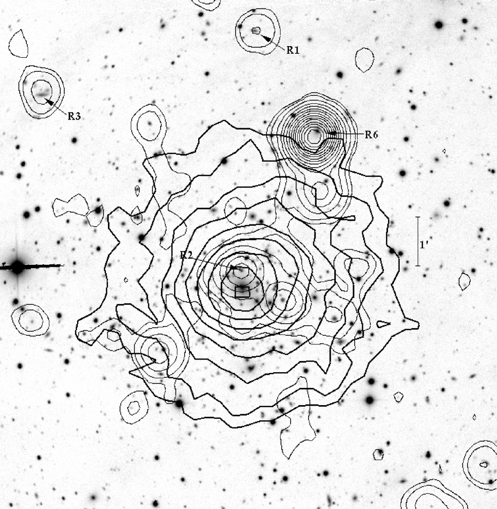
Figure 1: INT $R$–band image of the cluster A2294 (North at the top and East to the left) with, superimposed, the contour levels of the Chandra archival image ID 3246 (thick contours; photons in the energy range 0.5–2 keV) and the contour levels of a VLA radio image at 1.4 GHz (thin contours, see Giovannini et al. gio09 (2009)). Labels and arrows highlight the positions of radio sources listed by Rizza et al. (riz03 (2003)).

Unless otherwise stated, we give errors at the 68% confidence level (hereafter c.l.).

Throughout this paper, we use $H_{0}=70$ km s^-1 Mpc^-1 in a flat cosmology with $\Omega_{0}=0.3$ and $\Omega_{\Lambda}=0.7$. In the adopted cosmology, 1$\mathrm{{}^{\prime}}\;$corresponds to $\sim 173$ $h_{70}^{-1}$ kpc  at the cluster redshift.

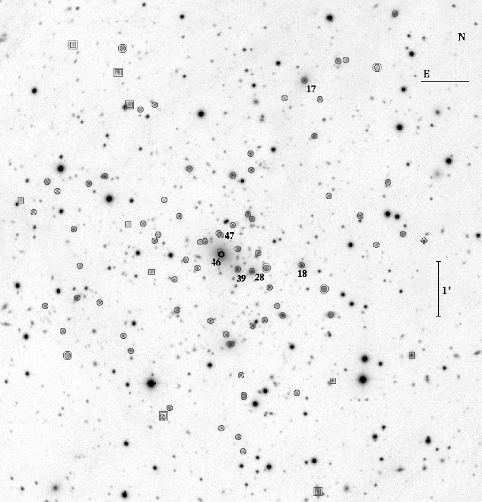
Figure 2: INT $R$–band image of the cluster A2294 (North at the top and East to the left). Circles and squares indicate cluster members and non–members, respectively (see Table 1). Solid circle in the center highlights the position of the BCG galaxy. Annuli and box annuli show member and non–member emission line galaxies, respectively. Labels indicate the IDs of cluster galaxies cited in the text. A diamond at the right border of the image highlights a QSO at $z\sim$2.1.

2 New data and galaxy catalog

Multi–object spectroscopic observations of A2294 were carried out at the TNG telescope in December 2007 and August 2008. We used DOLORES/MOS with the LR–B Grism 1, yielding a dispersion of 187 Å/mm. We used the new $2048\times 2048$ pixels E2V CCD, with a pixel size of 13.5 $\mu$m. In total we observed 4 MOS masks (3 in 2007 and 1 in 2008) for a total of 124 slits. We acquired three exposures of 1800 s for each mask. Wavelength calibration was performed using Helium–Argon lamps. Reduction of spectroscopic data was carried out with the IRAF package. Radial velocities were determined using the cross–correlation technique (Tonry & Davis ton79 (1979)) implemented in the RVSAO package (developed at the Smithsonian Astrophysical Observatory Telescope Data Center). Each spectrum was correlated against six templates for a variety of galaxy spectral types: E, S0, Sa, Sb, Sc, Ir (Kennicutt ken92 (1992)). The template producing the highest value of $\cal R$, i.e., the parameter given by RVSAO and related to the signal–to–noise ratio of the correlation peak, was chosen. Moreover, all spectra and their best correlation functions were examined visually to verify the redshift determination. In six cases (IDs. 5, 13, 15, 60, 81 and 82; see Table 1) we took the EMSAO redshift as a reliable estimate of the redshift.

Our spectroscopic survey in the field of A2294 consists of spectra for 88 galaxies.

Table 1: Velocity catalog of 88 spectroscopically measured galaxies in the field of the cluster A2294. ID 46, in boldface highlights the BCG. IDs in italics are non-member galaxies.

$$\begin{array}[]{r c c c r r l}\hline\cr\vskip 3.0pt plus 1.0pt minus 1.0pt\cr\hline\cr\vskip 3.0pt plus 1.0pt minus 1.0pt\cr\mathrm{ID}&\mathrm{\alpha},\mathrm{\delta}\,(\mathrm{J}2000)&B&R&\mathrm{v}&\mathrm{\Delta}\mathrm{v}&\mathrm{Emission}\\ &&&&\mathrm{(\,km}&\mathrm{s^{-1}\,)}&\mathrm{lines}\\ \hline\cr\vskip 3.0pt plus 1.0pt minus 1.0pt\cr\textit{1}&17\ 21\ 01.75,+85\ 51\ 21.1&18.65&17.21&28640&57&\\ 2&17\ 21\ 09.36,+85\ 53\ 32.7&19.79&17.82&51333&67&\\ 3&17\ 21\ 14.69,+85\ 57\ 31.3&19.04&16.92&52128&55&\\ 4&17\ 21\ 23.83,+85\ 54\ 29.0&20.24&18.17&51318&77&\\ 5&17\ 21\ 33.77,+85\ 56\ 33.5&20.29&19.42&48560&16&\mathrm{[OII]}\\ 6&17\ 21\ 35.57,+85\ 53\ 21.4&20.89&18.88&50550&71&\\ 7&17\ 21\ 52.15,+85\ 53\ 53.1&19.92&18.05&52312&59&\\ 8&17\ 22\ 05.21,+85\ 56\ 42.0&20.75&19.10&50779&147&\\ 9&17\ 22\ 13.44,+85\ 56\ 40.9&19.86&17.83&52063&59&\\ \textit{10}&17\ 22\ 20.83,+85\ 50\ 54.7&19.42&18.19&36167&77&\\ 11&17\ 22\ 22.49,+85\ 52\ 05.8&18.51&17.21&50279&109&\\ 12&17\ 22\ 23.50,+85\ 54\ 14.6&20.77&18.81&50787&66&\\ 13&17\ 22\ 29.06,+85\ 52\ 33.8&18.49&17.68&53150&75&\mathrm{[OII],H\beta}\\ 14&17\ 22\ 32.31,+85\ 55\ 59.5&20.97&18.83&51408&112&\\ \textit{15}&17\ 22\ 35.95,+85\ 48\ 54.6&18.56&17.22&21565&109&\mathrm{H\alpha}\\ 16&17\ 22\ 37.99,+85\ 55\ 19.7&19.55&17.54&49334&52&\\ 17&17\ 22\ 47.69,+85\ 56\ 20.1&18.87&16.64&49774&62&\\ 18&17\ 22\ 51.26,+85\ 52\ 59.6&18.99&16.89&51816&45&\\ 19&17\ 22\ 56.69,+85\ 50\ 41.1&20.57&18.79&49831&77&\\ 20&17\ 23\ 08.14,+85\ 56\ 01.1&21.08&19.14&50558&77&\\ 21&17\ 23\ 10.54,+85\ 52\ 05.5&19.02&17.04&50342&45&\\ 22&17\ 23\ 15.98,+85\ 52\ 16.1&20.84&18.94&48439&108&\\ 23&17\ 23\ 23.83,+85\ 52\ 35.9&19.98&17.89&54000&55&\\ 24&17\ 23\ 26.93,+85\ 52\ 56.8&19.06&18.06&53404&109&\mathrm{[OII],H\beta},\\ &&&&&&\mathrm{H\alpha,[NII]}\\ 25&17\ 23\ 28.63,+85\ 52\ 00.2&19.92&17.97&52231&60&\\ 26&17\ 23\ 35.18,+85\ 53\ 13.3&20.05&17.97&50231&54&\\ 27&17\ 23\ 40.37,+85\ 51\ 54.6&19.16&17.36&50708&66&\\ 28&17\ 23\ 41.37,+85\ 52\ 53.2&18.76&16.64&49068&34&\\ 29&17\ 23\ 41.47,+85\ 53\ 50.2&19.54&17.60&48114&64&\\ 30&17\ 23\ 41.73,+85\ 54\ 43.2&19.97&17.91&52330&48&\\ 31&17\ 23\ 42.82,+85\ 55\ 01.1&20.22&18.09&47906&70&\\ 32&17\ 23\ 45.34,+85\ 53\ 55.6&19.33&17.39&49027&52&\\ 33&17\ 23\ 49.32,+85\ 50\ 37.0&20.67&18.87&51693&113&\\ 34&17\ 23\ 49.37,+85\ 50\ 39.7&20.12&18.50&53475&57&\\ 35&17\ 23\ 49.78,+85\ 49\ 38.1&20.67&18.70&52794&99&\\ 36&17\ 23\ 52.46,+85\ 51\ 01.1&20.48&18.41&53149&59&\\ 37&17\ 23\ 54.51,+85\ 49\ 53.6&20.17&18.34&50294&77&\\ 38&17\ 23\ 55.53,+85\ 53\ 17.8&19.82&17.92&51367&104&\\ 39&17\ 23\ 55.92,+85\ 52\ 55.7&18.67&16.76&49221&41&\\ 40&17\ 24\ 00.51,+85\ 53\ 43.4&20.52&18.44&52927&78&\\ 41&17\ 24\ 00.91,+85\ 54\ 37.6&19.09&17.10&46553&60&\\ 42&17\ 24\ 01.54,+85\ 51\ 34.3&18.16&17.18&52055&31&\\ 43&17\ 24\ 03.53,+85\ 51\ 34.7&19.26&17.80&49876&69&\\ 44&17\ 24\ 06.91,+85\ 51\ 44.7&20.41&18.19&51991&69&\\ \vskip 3.0pt plus 1.0pt minus 1.0pt\cr\hline\cr\vskip 3.0pt plus 1.0pt minus 1.0pt\cr\hline\cr\end{array}$$

Table 1: Continued.

$$\begin{array}[]{r c c c r r l}\hline\cr\vskip 3.0pt plus 1.0pt minus 1.0pt\cr\hline\cr\vskip 3.0pt plus 1.0pt minus 1.0pt\cr\mathrm{ID}&\mathrm{\alpha},\mathrm{\delta}\,(\mathrm{J}2000)&B&R&\mathrm{v}&\mathrm{\Delta}\mathrm{v}&\mathrm{Emission}\\ &&&&\mathrm{(\,km}&\mathrm{s^{-1}\,)}&\mathrm{lines}\\ \hline\cr\vskip 3.0pt plus 1.0pt minus 1.0pt\cr 45&17\ 24\ 11.76,+85\ 50\ 03.4&20.91&19.00&51059&133&\\ \textbf{46}&17\ 24\ 12.14,+85\ 53\ 12.0&17.12&15.01&50671&66&\\ 47&17\ 24\ 12.94,+85\ 53\ 32.4&20.02&18.05&48983&71&\\ 48&17\ 24\ 13.62,+85\ 53\ 14.7&20.03&17.86&51068&186&\\ 49&17\ 24\ 14.94,+85\ 53\ 35.1&20.34&18.58&50477&101&\\ 50&17\ 24\ 22.95,+85\ 52\ 00.0&20.06&18.12&52427&97&\\ 51&17\ 24\ 28.34,+85\ 53\ 25.9&19.69&17.61&49638&63&\\ 52&17\ 24\ 33.43,+85\ 53\ 25.5&21.04&18.95&50207&74&\\ 53&17\ 24\ 36.29,+85\ 52\ 57.0&20.72&18.58&49332&88&\\ 54&17\ 24\ 44.81,+85\ 54\ 44.7&19.57&17.57&51597&76&\\ 55&17\ 24\ 48.05,+85\ 53\ 05.9&20.52&18.68&48339&76&\\ 56&17\ 24\ 54.51,+85\ 53\ 53.1&20.52&18.45&49696&70&\\ 57&17\ 24\ 55.99,+85\ 52\ 11.3&19.92&17.84&49614&85&\\ 58&17\ 24\ 59.28,+85\ 52\ 44.2&20.67&18.67&49486&56&\\ 59&17\ 25\ 03.41,+85\ 50\ 25.1&20.52&18.42&52052&74&\\ \textit{60}&17\ 25\ 09.21,+85\ 50\ 16.9&21.11&20.61&67190&313&\mathrm{[OII],H\beta},\\ &&&&&&\mathrm{[OIII]}\\ 61&17\ 25\ 09.98,+85\ 54\ 10.7&21.77&19.77&49754&104&\\ 62&17\ 25\ 10.31,+85\ 50\ 15.0&20.77&18.77&51675&218&\\ 63&17\ 25\ 15.91,+85\ 53\ 33.0&19.87&19.02&53186&66&\\ 64&17\ 25\ 19.18,+85\ 53\ 26.5&20.20&18.21&49892&116&\\ 65&17\ 25\ 19.99,+85\ 55\ 54.0&20.51&18.71&51267&113&\\ \textit{66}&17\ 25\ 22.27,+85\ 52\ 52.7&20.31&18.92&146216&80&\\ 67&17\ 25\ 31.13,+85\ 53\ 44.8&20.58&18.69&51558&57&\\ 68&17\ 25\ 34.97,+85\ 55\ 48.5&20.78&18.84&51215&67&\\ 69&17\ 25\ 42.63,+85\ 51\ 27.3&20.08&18.04&52589&70&\\ \textit{70}&17\ 25\ 45.98,+85\ 55\ 53.9&19.95&18.29&58151&92&\mathrm{[OII]}\\ \textit{71}&17\ 25\ 46.11,+85\ 53\ 44.3&21.58&19.96&81954&294&\\ 72&17\ 25\ 50.09,+85\ 51\ 43.2&20.54&18.58&52040&49&\\ 73&17\ 25\ 53.45,+85\ 56\ 55.0&19.77&18.66&48662&85&\mathrm{[OII],H\beta}\\ \textit{74}&17\ 25\ 57.79,+85\ 56\ 29.1&19.54&18.27&57854&111&\mathrm{[OII],H\beta}\\ 75&17\ 26\ 10.20,+85\ 54\ 35.9&19.31&17.25&50852&48&\\ 76&17\ 26\ 14.14,+85\ 52\ 19.3&20.50&18.59&50445&66&\\ 77&17\ 26\ 26.37,+85\ 54\ 27.9&19.78&17.83&51769&80&\\ 78&17\ 26\ 34.30,+85\ 52\ 58.7&20.37&18.76&47581&87&\\ 79&17\ 26\ 36.99,+85\ 52\ 23.7&18.83&17.04&49923&60&\\ 80&17\ 26\ 41.11,+85\ 53\ 38.2&19.93&18.02&49484&64&\\ \textit{81}&17\ 26\ 44.04,+85\ 56\ 58.2&21.52&19.85&89709&18&\mathrm{[OII]}\\ 82&17\ 26\ 45.34,+85\ 51\ 21.5&19.95&18.93&49890&64&\mathrm{[OII],H\beta},\\ &&&&&&\mathrm{[OIII],H\alpha}\\ 83&17\ 26\ 50.47,+85\ 51\ 47.5&20.52&18.71&49422&71&\\ 84&17\ 26\ 58.03,+85\ 54\ 19.1&20.69&18.93&52827&97&\\ 85&17\ 27\ 08.45,+85\ 52\ 14.8&20.66&18.60&51085&104&\\ 86&17\ 27\ 08.50,+85\ 54\ 29.4&19.54&17.99&48738&83&\\ 87&17\ 27\ 22.08,+85\ 53\ 56.5&20.38&18.82&52246&97&\\ \textit{88}&17\ 27\ 35.04,+85\ 54\ 08.7&21.18&18.98&90810&92&\\ \vskip 3.0pt plus 1.0pt minus 1.0pt\cr\hline\cr\vskip 3.0pt plus 1.0pt minus 1.0pt\cr\hline\cr\end{array}$$

The nominal errors as given by the cross–correlation are known to be smaller than the true errors (e.g., Malumuth et al. mal92 (1992); Bardelli et al. bar94 (1994); Ellingson & Yee ell94 (1994); Quintana et al. qui00 (2000)). Duplicate observations for the same galaxy allowed us to estimate real intrinsic errors in data of the same quality taken with the same instrument (e.g. Barrena et al. 2007a , 2007b ). Here we have a limited number of double determinations (i.e. five galaxies as coming from four different masks) thus we decided to apply the correction already applied in above studies. Hereafter we assume that true errors are larger than nominal cross–correlation errors by a factor 1.4. For the five galaxies with two redshift estimates we used the weighted mean of the two measurements and the corresponding errors.

The median error on $cz$ is 71 km s^-1.

As far as photometry is concerned, our observations were carried out with the Wide Field Camera (WFC), mounted at the prime focus of the 2.5m INT telescope. We observed A2294 in May 18th 2007 with filters $B_{\rm H}$ and $R_{\rm H}$ in photometric conditions and a seeing of $\sim$1.5$\mathrm{{}^{\prime}}\hskip-1.00006pt\mathrm{{}^{\prime}}$.

The WFC consists of a four–CCD mosaic covering a 33^′$\times$33$\mathrm{{}^{\prime}}\;$field of view, with only a 20% marginally vignetted area. We took nine exposures of 720 s in $B_{\rm H}$ and 360 s in $R_{\rm H}$ Harris filters (a total of 6480 s and 3240 s in each band) developing a dithering pattern of nine positions. This observing mode allowed us to build a “supersky” frame that was used to correct our images for fringing patterns (Gullixson gul92 (1992)). In addition, the dithering helped us to clean cosmic rays and avoid gaps between the CCDs in the final images. Another effect associated with the wide field frames is the distortion of the field. In order to match the photometry of several filters, a good astrometric solution is needed to take into account these distortions. Using the $imcoords$ IRAF tasks and taking as a reference the USNO B1.0 catalog, we were able to find an accurate astrometric solution (rms $\sim$0.4$\mathrm{{}^{\prime}}\hskip-1.00006pt\mathrm{{}^{\prime}}$) across the full frame. The photometric calibration was performed by observing standard Landolt fields (Landolt lan92 (1992)).

We finally identified galaxies in our $B_{\rm H}$ and $R_{\rm H}$ images and measured their magnitudes with the SExtractor package (Bertin & Arnouts ber96 (1996)) and AUTOMAG procedure. In a few cases (e.g. close companion galaxies, galaxies close to defects of the CCD) the standard SExtractor photometric procedure failed. In these cases we computed magnitudes by hand. This method consists in assuming a galaxy profile of a typical elliptical galaxy and scaling it to the maximum observed value. The integration of this profile gives us an estimate of the magnitude. This method is similar to PSF photometry, but assumes a galaxy profile, more appropriate in this case.

We transformed all magnitudes into the Johnson–Cousins system (Johnson & Morgan joh53 (1953); Cousins cou76 (1976)). We used $B=B\rm_{H}+0.13$ and $R=R\rm_{H}$ as derived from the Harris filter characterization (http://www.ast.cam.ac.uk/$\sim$wfcsur/technical/photom/colours/) and assuming a $B-V\sim 1.0$ for E–type galaxies (Poggianti pog97 (1997)). As a final step, we estimated and corrected the galactic extinction $A_{B}\sim 0.93$, $A_{R}\sim 0.58$ from Burstein & Heiles’s (bur82 (1982)) reddening maps. These values are especially high because A2294 is immersed in a diffuse dust cloud soaring high above the plane of our Milky Way Galaxy, and known as Polaris Dust Nebula.

We estimated that our photometric sample is complete down to $R=22.0$ (23.0) and $B=23.5$ (24.5) for $S/N=5$ (3) within the observed field.

We assigned magnitudes to all galaxies of our spectroscopic catalog.

Table 1 lists the velocity catalog (see also Fig. 2): identification number of each galaxy, ID (Col. 1); right ascension and declination, $\alpha$ and $\delta$ (J2000, Col. 2); $B$ and $R$ magnitudes (Cols. 3 and 4); heliocentric radial velocities, ${\rm v}=cz_{\sun}$ (Col. 5) with errors, $\Delta{\rm v}$ (Col. 6); emission lines detected in the spectra (Col. 7).

The brightest galaxy of A2294 (ID. 46 in Table 1, hereafter BCG) is a likely dominant galaxy, 1.6 $R$–magnitudes more luminous than other cluster members. The measured redshift is $z=0.1690\pm 0.0002$, different from that reported by Crawford et al. (cra95 (1995)), z=0.178, using INT data and measured on the H$\alpha$ emission line only. This discrepancy prompted us to acquire additional data for this galaxy. In August 2009 we acquired two 900 s exposure long–slit spectra of the BCG. We used the LR–R grism, covering the wavelength range $\sim$4500–10000 Å. The target was positioned in two slightly different positions of the slit in order to perform an optimal sky subtraction with a technique commonly used to reduce spectroscopic data in the near–infrared. Our reduced spectrum (see Fig. 3) does not show any evidence of the H$\alpha$ emission. Notice that the H$\alpha$ emission reported by Crawford et al. (cra95 (1995)) is very strong $\rm EW_{H\alpha}=51.7\pm 3.2$ (see for comparison the spectrum of A291 having $\rm EW_{H\alpha}=20.9\pm 0.9$ in their Fig. 1) and thus its presence would be just striking in our spectrum. Indeed, we strongly suspect that their detection is due to some problem in data reduction, e.g. a cosmic ray or sky subtraction, as also suggested by the wrong measure of the galaxy redshift.

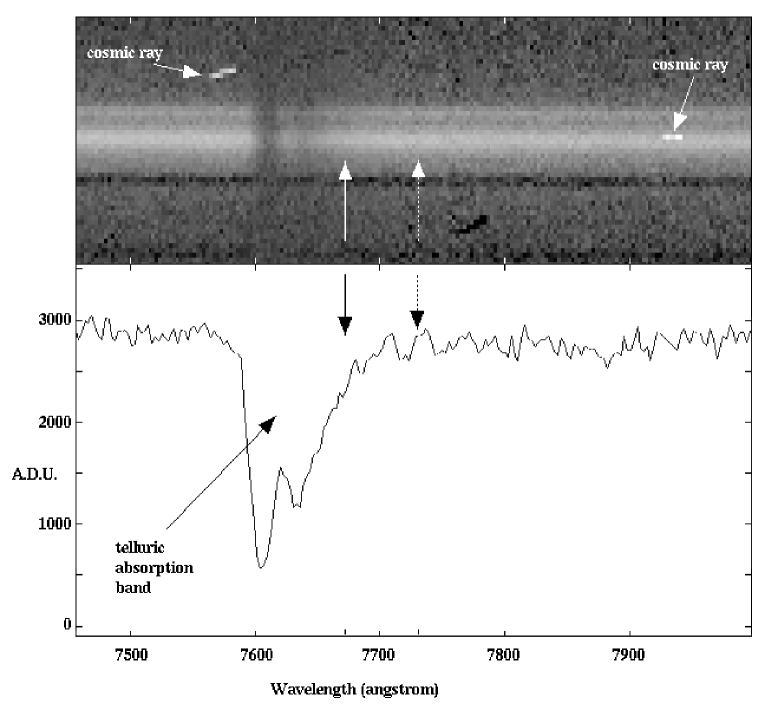
Figure 3: Top panel: 2D spectrum of the BCG galaxy taken with the grism LR–R mounted on DOLORES in the wavelength range $\sim$7500–8000 Å. Bottom panel: 1D reduced spectrum of the BCG galaxy in the same wavelength range as above. Solid and dashed arrows indicate the position of the (hypothetical) H$\alpha$ emission line according to the redshift given in this paper and to the redshift provided by Crawford et al. (cra95 (1995)), respectively. The spectrum does not show any evidence of the H$\alpha$ emission.

Other cluster members are much less luminous than the BCG: out of them, the brightest ones lie in the central cluster region (IDs. 28, 39 and 18) with the exception of ID. 17 (hereafter R6) which lies in the northern region and is very radio luminous ($>10^{24}$ W Hz^-1, No. 6 of Rizza et al. riz03 (2003)). Out of radio galaxies listed by Rizza et al. riz03 (2003)), we have also acquired redshift for their No. 2 (ID. 47, labelled as R2 in Fig. 1), confirming its membership to the cluster.

3 Analysis of the spectroscopic sample

3.1 Member selection

To select cluster members out of 88 galaxies having redshifts, we follow a two steps procedure. First, we perform the 1D adaptive–kernel method (hereafter DEDICA, Pisani pis93 (1993) and pis96 (1996); see also Fadda et al. fad96 (1996); Girardi et al. gir96 (1996)). We search for significant peaks in the velocity distribution at $>$99% c.l.. This procedure detects A2294 as a peak at $z\sim 0.169$ populated by 80 galaxies considered as candidate cluster members (in the range $46553\leq{\rm v}\leq 58151$, see Fig. 4). Out of eight non–members, three and five are foreground and background galaxies, respectively.

Figure 4: Redshift galaxy distribution. The solid line histogram refers to the 80 galaxies assigned to the A2294 complex according to the DEDICA reconstruction method. The number-galaxy density in the redshift space, as provided by the adaptive kernel reconstruction method is overlapped to the histogram.

All the galaxies assigned to the cluster peak are analyzed in the second step which uses the combination of position and velocity information: the “shifting gapper” method by Fadda et al. (fad96 (1996)). This procedure rejects galaxies that are too far in velocity from the main body of galaxies within a fixed bin that shifts along the distance from the cluster center. The procedure is iterated until the number of cluster members converges to a stable value. Following Fadda et al. (fad96 (1996)) we use a gap of $1000$ km s${}^{-1}\;$– in the cluster rest–frame – and a bin of 0.6 $h_{70}^{-1}$ Mpc, or large enough to include 15 galaxies. As for the center of A2294 we adopt the position of the BCG [R.A.=$17^{\mathrm{h}}24^{\mathrm{m}}12\,\hbox to0.0pt{\hbox{$\mathrm{{}^{s}}$}\hss}{\hbox{$.$}}\,14$, Dec.=$+85\mathrm{{}^{\circ}}53\mathrm{{}^{\prime}}12\mathrm{{}^{\prime}}\hskip-1.00006pt\mathrm{{}^{\prime}}\;$ (J2000.0)], which is almost coincident to the X-ray centroid obtained in this paper using Chandra data (see Sect. 4). The “shifting gapper” procedure rejects other two obvious interlopers very far from the main body ($>2000$ km s^-1) but survived to the first step of our member selection procedure. We obtain a sample of 78 fiducial members (see Fig. 5).

Figure 5: The 78 galaxies assigned to the cluster. Upper panel: Velocity distribution. The arrows indicate the velocities of the five brightest galaxies, in particular we indicate the brightest cluster galaxy “BCG”, the bright radio galaxy “R6”. Lower panel: Stripe density plot where the arrows indicate the positions of the significant gaps.

The five member galaxies showing emission lines (ELGs) are preferentially found in the external cluster regions (see Fig. 2). The only ELG close to the cluster center (ID. 24) lies in the high tail of the velocity distribution, far more than $cz=2500$ km s${}^{-1}\;$from the mean cluster velocity, as expected e.g. in the case of a very radial orbit. These findings are in general agreement with large statistical analyses of ELGs in clusters (see Biviano et al. biv97 (1997) and refs. therein).

3.2 Global cluster properties

By applying the biweight estimator to the 78 cluster members (Beers et al. bee90 (1990), ROSTAT software), we compute a mean cluster redshift of $\left<z\right>=0.1693\pm$ 0.0005, i.e. $\left<\rm{v}\right>=(50769\pm$155) km s^-1. We estimate the LOS velocity dispersion, $\sigma_{\rm V}$, by using the biweight estimator and applying the cosmological correction and the standard correction for velocity errors (Danese et al. dan80 (1980)). We obtain $\sigma_{\rm V}=1363_{-91}^{+110}$ km s^-1, where errors are estimated through a bootstrap technique.

To evaluate the robustness of the $\sigma_{\rm V}$ estimate we analyze the velocity dispersion profile (Fig. 6). The integral profile rises out to $\sim 0.2$ $h_{70}^{-1}$ Mpc and then flattens suggesting that a robust value of $\sigma_{\rm V}$ is asymptotically reached in the external cluster regions, as found for most nearby clusters (e.g., Fadda et al. fad96 (1996); Girardi et al. gir96 (1996)).

Figure 6: Top panel: rest–frame velocity vs. projected distance from the cluster center. Squares indicate the five brightest galaxies. Middle and bottom panels: differential (big circles) and integral (small points) profiles of mean velocity and LOS velocity dispersion, respectively. For the differential profiles we plot the values for five annuli from the center of the cluster, each of 0.25 $h_{70}^{-1}$ Mpc (large symbols). For the integral profiles, the mean and dispersion at a given (projected) radius from the cluster–center is estimated by considering all galaxies within that radius – the first value computed on the five galaxies closest to the center. The error bands at the $68\%$ c.l. are also shown. In the lower panel, the horizontal line represents the X–ray temperature (see Sect. 4) with the respective errors transformed in $\sigma_{\rm V}$ assuming the density–energy equipartition between ICM and galaxies, i.e. $\beta_{\rm spec}=1$ (see Sect. 5).

In the framework of usual assumptions (cluster sphericity, dynamical equilibrium, coincidence of the galaxy and mass distributions), one can compute virial global quantities. Following the prescriptions of Girardi & Mezzetti (gir01 (2001)), we assume for the radius of the quasi–virialized region ${\rm R}_{\rm vir}=0.17\times\sigma_{\rm V}/H(z)=3.05$ $h_{70}^{-1}$ Mpc – see their eq. 1 with the scaling with $H(z)$ (see also eq.  8 of Carlberg et al. car97 (1997) for ${\rm R}_{200}$). We compute the virial mass (Limber & Mathews lim60 (1960); see also, e.g., Girardi et al. gir98 (1998)):

$$M=3\pi/2\cdot\sigma_{\rm V}^{2}{\rm R}_{\rm PV}/G-{\rm SPT},$$ (1)

where SPT is the surface pressure term correction (The & White the86 (1986)), and ${\rm R}_{\rm PV}$ is a projected radius (equal to two times the projected harmonic radius).

The estimate of $\sigma_{\rm V}$ is robust when computed within a large cluster region (see Fig. 6). The value of ${\rm R}_{\rm PV}$ depends on the size of the sampled region and possibly on the quality of the spatial sampling (e.g., whether the cluster is uniformly sampled or not). Since in A2294 we have sampled only a fraction of ${\rm R}_{\rm vir}$, we have to use an alternative estimate of ${\rm R}_{\rm PV}$ on the basis of the knowledge of the galaxy distribution. Following Girardi et al. (gir98 (1998); see also Girardi & Mezzetti gir01 (2001)) we assume a King–like distribution with parameters typical of nearby/medium–redshift clusters: a core radius ${\rm R}_{\rm c}=1/20\times{\rm R}_{\rm vir}$ and a slope–parameter $\beta_{\rm fit,gal}=0.8$, i.e. the volume galaxy density at large radii goes as $r^{-3\beta_{fit,gal}}=r^{-2.4}$. We obtain ${\rm R}_{\rm PV}(<{\rm R}_{\rm vir})=2.27$ $h_{70}^{-1}$ Mpc, where a $25\%$ error is expected (Girardi et al. gir98 (1998), see also the approximation given by their eq. 13 when $A={\rm R}_{\rm vir}$). The value of SPT strongly depends on the radial component of the velocity dispersion at the radius of the sampled region and could be obtained by analyzing the (differential) velocity dispersion profile, although this procedure would require several hundred galaxies. We decide to assume a $20\%$ SPT correction as obtained in the literature by combining data on many clusters sampled out to about ${\rm R}_{\rm vir}$ (Carlberg et al. car97 (1997); Girardi et al. gir98 (1998)). We compute $M(<{\rm R}_{\rm vir}=3.05\;h_{70}^{-1}\mathrm{Mpc})=3.7_{-1.0}^{+1.1}$ $\times 10^{15}\;h_{70}^{-1}\;M_{\odot}$.

3.3 Velocity distribution

We analyze the velocity distribution to look for possible deviations from Gaussianity that might provide important signatures of complex dynamics. For the following tests the null hypothesis is that the velocity distribution is a single Gaussian.

We estimate three shape estimators, i.e. the kurtosis, the skewness, and the scaled tail index (see, e.g., Beers et al. bee91 (1991)). We find no evidence that the velocity distribution departs from Gaussianity.

Then we investigate the presence of gaps in the velocity distribution. We follow the weighted gap analysis presented by Beers et al. (bee91 (1991); bee92 (1992); ROSTAT software). We look for normalized gaps larger than 2.25 since in random draws of a Gaussian distribution they arise at most in about $3\%$ of the cases, independent of the sample size (Wainer and Schacht wai78 (1978)). We detect two significant gaps (at the $97\%$ and $98.6\%$ c.l.s) which divide the cluster in three groups of 28, 14 and 36 galaxies from low to high velocities (hereafter GV1, GV2 and GV3, see Fig. 5). The BCG is assigned to the GV2 peak. Among other luminous galaxies, R6, IDs. 28 and 39 are assigned to the GV1 peak and ID. 18 to the GV3 peak.

Following Ashman et al. (ash94 (1994)) we also apply the Kaye’s mixture model (KMM) algorithm. This test does not find a three–groups partition which is a significantly better descriptor of the velocity distribution with respect to a single Gaussian.

3.4 3D–analysis

The existence of correlations between positions and velocities of cluster galaxies is a footprint of real substructures. Here we use three different approaches to analyze the structure of A2294 combining position and velocity information.

To look for a possible physical meaning of the three subclusters determined by the two weighted gaps we compare two by two the spatial galaxy distributions of GV1, GV2, and GV3. We find that the GV1 and GV3 groups differ in the distributions of the clustercentric distances of member galaxies at the $93\%$ c.l. (according to the the 1D Kolmogorov–Smirnov test; hereafter 1DKS–test, see e.g., Press et al. pre92 (1992)). The GV1 galaxies are, on average, closer to the cluster center than the GV3 galaxies (see Fig. 7).

Figure 7: Spatial distribution on the sky of the cluster galaxies showing the three groups recovered by the weighted gap analysis. Solid circles, crosses and open circles indicate the galaxies of GV1, GV2 and GV3, respectively. The BCG is taken as the cluster center. Large squares indicate the five brightest cluster members. Among them, the BCG and R6 are indicated by the two largest squares.

We analyze the presence of a velocity gradient performing a multiple linear regression fit to the observed velocities with respect to the galaxy positions in the plane of the sky (e.g, Boschin et al. bos04 (2004) and refs. therein). We find a position angle on the celestial sphere of $PA=214_{-28}^{+33}$ degrees (measured counter–clock–wise from north), i.e. higher–velocity galaxies lie in the SSW region of the cluster. To assess the significance of this velocity gradient we perform 1000 Monte Carlo simulations by randomly shuffling the galaxy velocities and for each simulation we determine the coefficient of multiple determination ($RC^{2}$, see e.g., NAG Fortran Workstation Handbook nag86 (1986)). We define the significance of the velocity gradient as the fraction of times in which the $RC^{2}$ of the simulated data is smaller than the observed $RC^{2}$. We find that the velocity gradient is marginally significant at the $91\%$ c.l..

We also combine galaxy velocity and position information to compute the $\Delta$–statistics devised by Dressler & Schectman (dre88 (1988); see also e.g., Boschin et al. bos06 (2006) for a recent application). We find no significant indication of substructure.

3.5 Kinematics of more luminous galaxies

The presence of velocity segregation of galaxies with respect to their colors, luminosities, and morphologies is often taken as evidence of advanced dynamical evolution of the parent cluster (e.g. Biviano et al. biv92 (1992); Fusco-Femiano & Menci fus98 (1998)). Here we check for possible luminosity segregation of galaxies in the velocity space.

We find no significant correlation between the absolute velocity $|{\rm v}|$ and $R$–magnitude. We also divide the sample in a low and a high–luminosity subsamples by using the median $R$–magnitude=18.145. The two subsamples do not differ in their velocity distribution as we verify with the standard means–test and F–test (e.g., Press et al. pre92 (1992)) applied to the means and variances of velocities and with the 1DKS–test applied to the whole velocity distributions. This is in agreement with the very small range of action of velocity segregation in galaxy clusters, i.e. typically only the three most luminous galaxies (Biviano et al. biv92 (1992); see also Goto got05 (2005)).

Examining the velocity distributions of the two subsamples in more details we find that the distribution of luminous galaxies is found to be non–Gaussian according to the scale tail index (at the $95\%$ c.l.) and that, according to the 1D–DEDICA technique, it is better described by a bimodal distribution (see Fig. 8). The two peaks of this distribution, of 20 and 19 galaxies at $\sim 49700$ and 51950 km s${}^{-1}\;$respectively, are separated by $\sim 2000$ km s${}^{-1}\;$in the rest cluster frame and appear largely overlapped, i.e. 15 galaxies have a non–null probability to belong to both the peaks. The BCG is assigned to the low–velocity peak, but with a large probability to belong to the other peak. Among other luminous galaxies, R6, IDs. 28 and 39 are assigned to the low–velocity peak and ID. 18 to the high–velocity peak.

Figure 8: Velocity galaxy distribution of more and less luminous cluster members (solid and dashed lines, respectively). The arrows indicate the velocities of the five brightest galaxies, in particular “BCG” indicates the bright, central galaxy and “R6” indicates the bright radio–galaxy. The number-galaxy densities, as provided by the adaptive kernel reconstruction method are overlapped to the histograms.

According to the DEDICA assignment, we estimate $\sigma_{\rm V}\sim 780$ and $\sim 640$ km s${}^{-1}\;$for the low and high-velocity groups, respectively. However, since there is a wide velocity–range where galaxies have a non–zero probability of belonging to both the clumps, DEDICA membership assignment leads to an artificial truncation of the of the tails of the distributions. This truncation may lead to an underestimate of velocity dispersion for the subclusters. Thus, we prefer to rely on the estimates obtained through the KMM approach even if the best bimodal fit is not a significant improvement with respect to the single Gaussian according to the likelihood ratio test. The low– and high–velocity groups given by the best KMM bimodal fit have mean velocities $\left<\rm{v}\right>\sim 49740$ and 52230 km s^-1, in good agreement with the peak velocities reported above and $\sigma_{\rm V}\sim 1070$ and $\sim 670$ km s^-1.

3.6 Analysis of the photometric sample

By applying the 2D adaptive–kernel method to the positions of A2294 galaxy members we find only one significant peak. However, our spectroscopical data do not cover the entire cluster field and suffer of magnitude incompleteness. To overcome these limits we recover our photometric catalog selecting likely members on the basis of the color–magnitude relation (hereafter CMR), which indicates the early–type galaxy locus. To determine the CMR we fix the slope according to López–Cruz et al. (lop04 (2004), see their Fig. 3) and apply the two–sigma–clipping fitting procedure to the cluster members obtaining $B$–$R=3.185-0.066\times R$ (see Fig. 9). Out of our photometric catalog we consider as likely cluster members those objects with a SExtractor stellar index $\leq 0.9$ lying within 0.25 mag of the CMR. To avoid contamination by field galaxies we do not show results for galaxies fainter than 21 mag (in $R$–band). Figure 10 shows the contour map for the likely cluster members having $R\leq 21$: we find again that A2294 is well described by only one peak centered on the BCG galaxy.

Figure 9: $B$–$R$ vs. $R$ diagram for galaxies with available spectroscopy is shown by circles and crosses (cluster and field members, respectively). The solid line gives the best–fit color–magnitude relation as determined on member galaxies; the dashed lines are drawn at $\pm$0.25 mag from the CMR.

Figure 10: Spatial distribution on the sky and relative isodensity contour map of likely cluster members extracted from our photometric catalog with $R\leq 21$. The contour map is obtained with the DEDICA method (black lines). The plot is centered on the cluster center.

4 X–ray analysis

The X–ray analysis of A2294 is performed on the archival data of the Chandra ACIS–I observation 800246 (exposure ID #3246). The pointing has an exposure time of 10 ks. Data reduction is performed using the package CIAO (Chandra Interactive Analysis of Observations, ver. 3.3 with CALDB ver. 3.2.1) on chips I0, I1, I2 and I3 (field of view $\sim 17\arcmin\times 17\arcmin$). First, we remove events from the level 2 event list with a status not equal to zero and with grades one, five and seven. Then, we select all events with energy between 0.3 and 10 keV. In addition, we clean bad offsets and examine the data, filtering out bad columns and removing times when the count rate exceeds three standard deviations from the mean count rate per 3.3 s interval. We then clean the four chips for flickering pixels, i.e., times where a pixel has events in two sequential 3.3 s intervals. The resulting exposure time for the reduced data is 9.9 ks.

A quick look at the reduced image is sufficient to reveal the regular morphology of the extended X–ray emission of this cluster (see Fig. 11). The low values of the $P_{\rm m}/P_{0}$ power ratios found by Bauer et al. (bau05 (2005)) quantitatively support this feeling. The absence of multiple clumps in the ICM is confirmed by performing a wavelet multiscale analysis on the chip I3. In fact, the task CIAO/Wavdetect identifies A2294 as a single extended X–ray source.

To better characterize the X–ray morphology of the cluster, by using the CIAO package Sherpa we fit a simple Beta model to the 2D X–ray photon distribution on the chip I3. The model is defined as follows (Cavaliere & Fusco–Femiano cav76 (1976)):

$$S({\rm R})=S_{0}[1+({\rm R}/{\rm R}_{\rm c})^{2}]^{\alpha}+b,$$ (2)

where $\rm R$ is the projected radial coordinate from the centroid position and $b$ the surface brightness background level. Before the fit we binned the image by a factor 8 and divided it by a normalized exposure map. The best fit centroid position is located at R.A.=$17^{\mathrm{h}}24^{\mathrm{m}}04\,\hbox to0.0pt{\hbox{$\mathrm{{}^{s}}$}\hss}{\hbox{$.$}}\,87$ and Dec.=$+85\mathrm{{}^{\circ}}53\mathrm{{}^{\prime}}15.6\mathrm{{}^{\prime}}\hskip-1.00006pt\mathrm{{}^{\prime}}\;$ (J2000.0, with an error of $\pm 0.8\mathrm{{}^{\prime}}\hskip-1.00006pt\mathrm{{}^{\prime}}$) at $\sim$8.5$\mathrm{{}^{\prime}}\hskip-1.00006pt\mathrm{{}^{\prime}}\;$from the position of the BCG. The slope parameter is $\alpha$=-0.96$\pm$0.05, that is $\beta_{\rm fit,gas}=(-\alpha+0.5)/3=0.49\pm 0.02$, and the (angular) core radius is R${}_{\rm c}=36.2\mathrm{{}^{\prime}}\hskip-1.00006pt\mathrm{{}^{\prime}}\;_{-2.5\mathrm{{}^{\prime}}\hskip-0.70004pt\mathrm{{}^{\prime}}\;}^{+2.7\mathrm{{}^{\prime}}\hskip-0.70004pt\mathrm{{}^{\prime}}\;}$. At the redshift of A2294 the core radius corresponds to 104.4${}^{+7.7}_{-7.3}$ $h_{70}^{-1}$ kpc.

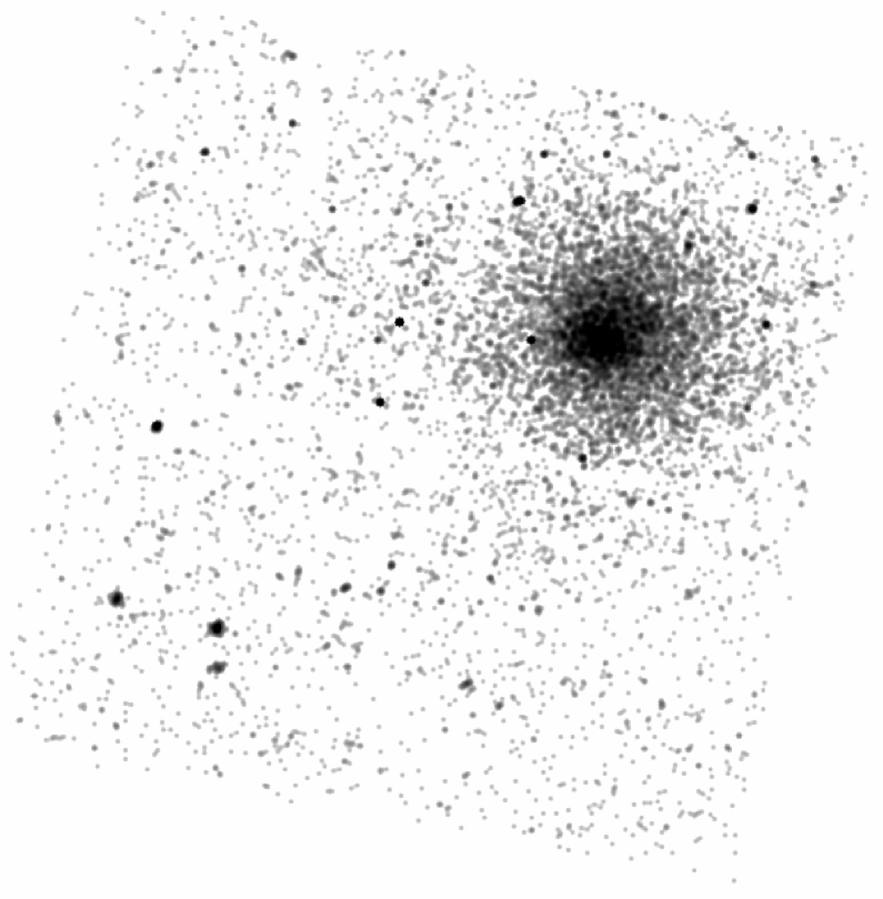
Figure 11: 17^′$\times$17$\mathrm{{}^{\prime}}\;$Chandra X–ray smoothed image (ID 3246) of A2294 in the energy band 0.5–2 keV (North at the top and East to the left).

The above model is an adequate description fit to the data (the reduced CSTAT statistic is 1.04; Cash cas79 (1979)). However, we check for possible departures of the X–ray surface brightness, and thus of the gas density distribution, from the Beta model fit by investigating the Beta model residuals. The residuals show a deficit of X–ray emitting gas in a region extending along the NE–SW direction, with a negative peak in the very central cluster region (see Fig. 12). Around the cluster center, elongated in the direction SE–NW, there are also regions with excess of positive residuals.

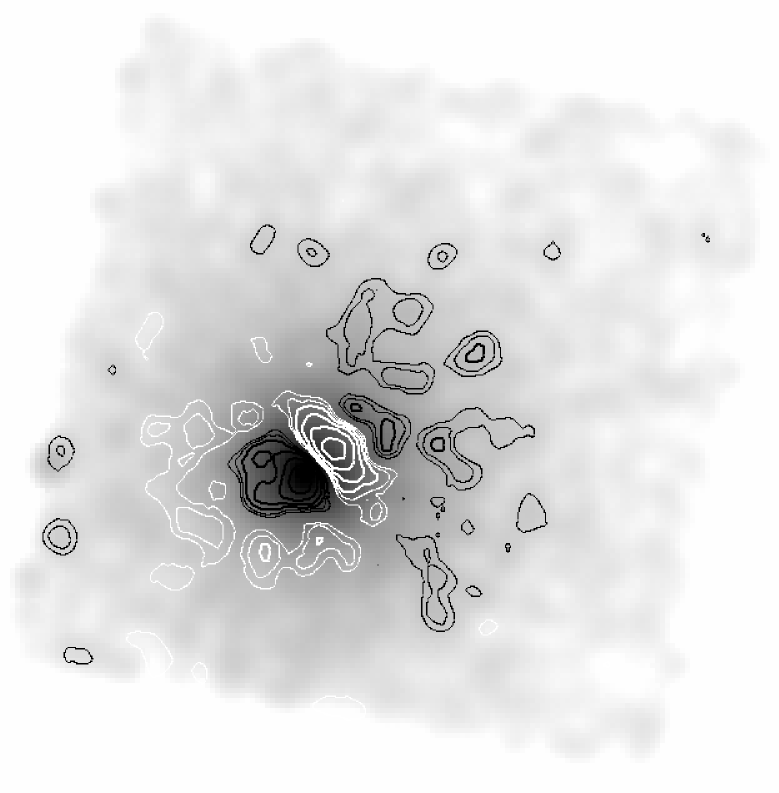
Figure 12: T

he smoothed X–ray emission in the right-upper quadrant of Fig. 11 with, superimposed, the contour levels of the positive (black) and negative (white) smoothed Beta model residuals (North at the top and East to the left).

As for the spectral properties of the cluster X–ray photons, we compute a global estimate of the ICM temperature. The temperature is computed from the X–ray spectrum of the cluster within a circular aperture of $\sim$173$\mathrm{{}^{\prime}}\hskip-1.00006pt\mathrm{{}^{\prime}}\;$radius (0.5 $h_{70}^{-1}$ Mpc at the cluster redshift) around the centroid of the X–ray emission. Fixing the absorbing galactic hydrogen column density at 6.19$\times$10²⁰ cm^-2, computed from the HI maps by Dickey & Lockman (dic90 (1990)), we fit a Raymond–Smith (ray77 (1977)) spectrum using the CIAO package Sherpa with a $\chi^{2}$ statistics and assuming a metal abundance of 0.3 in solar units. We find a best fitting temperature of $T_{\rm X}=\,$10.3 $\pm\,1.1$ keV.

A detailed temperature and metallicity map would be highly desirable to better describe the properties of the ICM, but due to the relatively small exposure time the photon statistics is not good enough to this aim. However, a low SNR option to detect possible temperature gradients in the ICM is producing a “hardness” (or “softness”) map of the cluster. We create two images in the energy bands 0.5–2 keV (soft band) and 2–7 keV (hard band), subtracting a constant background level in each energy band. Computing counts in the soft ($S$) and in the hard ($H$) band we define the quantity “softness ratio” as $SR=(S-H)/(S+H)$. Both images are exposure-corrected with their corresponding exposure maps. The low number of photons available force us to choose a large pixel size in order to get a good count statistic per pixel, so the resolution of the soft and hard images is low (182 kpc pix^-1). A 3D graph of the $SR$ values in the pixels within a radius of 0.5 $h_{70}^{-1}$ Mpc from the cluster center is reported in Fig. 13. Typical errors are $\pm 0.4$, while the median value of $SR$ is 0.25. According to the PIMMS tool this value corresponds to a temperature of $\sim 9.7$ keV, in good agreement with the global temperature reported above. The $SR$ 3D graph does not show any evidence of significant temperature gradients.

13

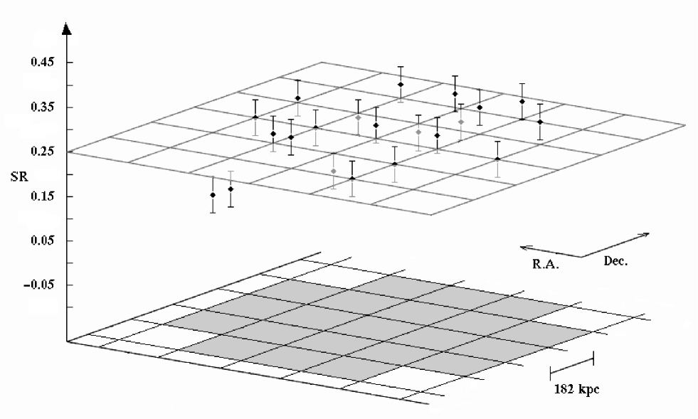
Figure 13: Softness ratio 3D map of A2294 around the centroid of the X–ray distribution. The plane at the median $SR$ value (0.25) is drawn.

5 Discussion and conclusions

Our estimate of the cluster redshift is $\left<z\right>=0.1693\pm$ 0.0005 and the BCG is well at rest within the cluster (cfr. our $z=0.1690$ with $z=0.178$ by Crawford et al. cra95 (1995)).

For the first time the internal dynamics of A2294 is analyzed.

The high values of the velocity dispersion $\sigma_{\rm V}=1363_{-91}^{+110}$ km s${}^{-1}\;$and X–ray temperature $T_{\rm X}=(10.3\pm 1.1)$ keV are comparable to the highest values found in typical clusters (see Mushotzky & Scharf mus97 (1997); Girardi & Mezzetti gir01 (2001); Leccardi & Molendi lec08 (2008)). Our estimates of $\sigma_{\rm V}$ and $T_{\rm X}$ are fully consistent when assuming the equipartition of energy density between ICM and galaxies. In fact, we obtain $\beta_{\rm spec}=1.09^{+0.18}_{-0.15}$ to be compared with $\beta_{\rm spec}=1$, where $\beta_{\rm spec}=\sigma_{\rm V}^{2}/(kT/\mu m_{\rm p})$ with $\mu=0.58$ the mean molecular weight and $m_{\rm p}$ the proton mass (see also Fig. 6). Taking on face this result one might think that A2294 is not far from dynamical equilibrium and consider very reliable the virial mass estimate $M(<{\rm R}_{\rm vir}\sim 3\;h_{70}^{-1}\mathrm{Mpc})\sim 4$ $\times 10^{15}\;h_{70}^{-1}\;M_{\odot}\;$computed in § 3.2.

5.1 Internal structure

However, our analysis shows signs that this cluster is not so relaxed as one can think at a first glance. Evidence in this sense comes from both optical and X–ray analyses.

First of all, both the integral and differential velocity dispersion profiles rise in the central region out to $\sim 0.2$ $h_{70}^{-1}$ Mpc (Fig. 6, middle and bottom panels). As for the velocity dispersion, this behavior might be a signature of a relaxed cluster due to circular velocities and galaxy mergers phenomena in the central cluster region (e.g., Merritt mer88 (1988); Menci & Fusco Femiano men96 (1996); Girardi et al. gir98 (1998)). Alternatively, it might be due to the presence of subclumps, having different mean velocities (see, e.g., Abell 3391–3395 in Girardi et al. gir96 (1996); Abell 115 in Barrena et al. 2007b ). The latter hypothesis is supported by the behavior of the mean velocity profile and by the plot of velocity vs. projected clustercentric distance where the central region is more populated by low velocity galaxies than high velocity galaxies. This suggests the presence of substructure in the cluster core.

Second, the two gaps found in the velocity distribution suggest the presence of three subclumps with the BCG in the middle velocity subclump. Although the presence of the three groups (GV1, GV2, GV3) is not very strongly significant on the base of only velocity data, the existence of a spatial segregation between GV1 and GV3 groups is a footprint of real substructures. We also find a (marginally significant) velocity gradient toward the SSW direction.

Third, the high–luminosity galaxy subsample shows two peaks (largely overlapped) in the velocity distribution, with the BCG someway in the middle. This result is very appealing, since galaxies of different luminosity could trace the dynamics of cluster mergers in a different way. A noticeable example was reported by Biviano et al. (biv96 (1996)): they found that the two central dominant galaxies of the Coma cluster are surrounded by luminous galaxies, accompanied by the two main X–ray peaks, while the distribution of faint galaxies tend to form a structure not centered with one of the two dominant galaxies, but rather coincident with a secondary peak detected in X–ray. Biviano et al. speculate that the merging is in an advanced phase, where faint galaxies trace the forming structure of the cluster, while the most luminous galaxies still trace the remnant of the core–halo structure of a pre–merging clump, which could be so dense to survive for a long time after the merging (as suggested by numerical simulations, e.g. González–Casado et al. gon94 (1994)). In A2294, we can speculate that luminous galaxies trace the remnants of two merging subclusters characterized by an impact velocity $\sim$ 2000 km s^-1. Assuming the dynamical equilibrium for each of the two individual subclusters, from the values of $\sigma_{\rm V}$ of the two subclusters we obtain a virial mass of 1.8 $\times 10^{15}\;h_{70}^{-1}\;M_{\odot}\;$and 0.5 $\times 10^{15}\;h_{70}^{-1}\;M_{\odot}\;$for the low and high velocity subclusters. The total mass $M_{\rm sys}=2.3$ $\times 10^{15}\;h_{70}^{-1}\;M_{\odot}\;$is lower than the global virial value computed in § 3.2, but still a high value.

As for X–ray data, we find no evidence of obvious substructure. In fact, our multiscale wavelet analysis of the Chandra image does not reveal any subclumps in the X–ray photon distribution. Moreover, we confirm the absence of a significant, macroscopic cluster ellipticity (see also Hashimoto et al. has07 (2007); Maughan et al. mau08 (2008)).

As for the Beta model we fit, the value of the core radius R${}_{\rm c}=104.4^{+7.7}_{-7.3}$ $h_{70}^{-1}$ kpc  and the value of the slope parameter $\beta_{\rm fit,gas}=0.49\pm 0.03$ well agree with those computed by Hart in his PhD thesis (har08 (2008); R${}_{\rm c}=(99\pm 12)$ $h_{70}^{-1}$ kpc; $\beta_{\rm fit,gas}=0.48\pm 0.02$). The value of the core radius agrees with that expected from the relation between surface brightness concentration index and core radius shown by Hashimoto et al. (has07 (2007), see their Fig. 8 and the value of concentration in their Table 2). The values of R_c and $\beta_{\rm fit,gas}$ well lie on the low end of the parabolic relation found between these two parameters (Neumann & Arnaud neu99 (1999)). On the other hand, the value of $\beta_{\rm fit,gas}=0.49\pm 0.03$ might seem somewhat small considering the typical values for very rich/hot clusters (e.g., Jones & Forman jon99 (1999); Vikhlinin et al. vik99 (1999)). However, notice that most our signal comes from the region with a radius of $\sim 0.5$ $h_{70}^{-1}$ Mpc ($\sim 1/6\,{\rm R_{vir}}$) and that there are indications for continuous steepening of the X–ray brightness profiles with increasing radius (e.g., Vikhlinin et al. vik99 (1999); Neumann neu05 (2005)). This steepening is the likely cause of offsets between different cluster samples (see Vikhlinin et al. vik99 (1999) where $\beta_{\rm fit,gas}\gtrsim 0.6$ vs. Jones & Forman jon99 (1999) where $\left<\beta_{\rm fit,gas}\right>=0.6$) and of apparent discrepancies between fit parameters obtained for the same clusters (e.g. Buote et al. buo05 (2005)). Indeed, the most appropriate way to compare different clusters it seems to consider the measure of the local slope of the surface brightness at a certain, rescaled radius (see Croston et al. cro08 (2008) for variation of this parameter with radius). As for A2294, Maughan et al. (mau08 (2008)) computed the slope $\beta_{500}=1.22^{+0.32}_{-0.25}$ at a radius of R${}_{500}=1.3$ $h_{70}^{-1}$ Mpc, using the data in the radial range 0.7R₅₀₀-1.3R₅₀₀, i.e. well out of the region we analyze. This value is in agreement with that expected for very hot clusters at $z<0.5$ (see their Fig. 11). Finally, we notice that, in the case of a cluster merger, numerical simulations predict a clear expansion of the gas core and a somewhat steepening of the slope (Roettiger et al. roe96 (1996), see their Fig. 3). This is in agreement with that suggested by Jones & Forman (jon99 (1999)) to explain the large core radii found for a few observed clusters, but see Neumann & Arnaud (neu99 (1999)) for no link between $\beta_{\rm fit,gas}$ value and cluster dynamical status. Summarizing, our small values of R_c and $\beta_{\rm fit,gas}$ are not suggestive of substructure.

Direct evidence of cluster substructure comes from the 2D image of the Beta model residuals, which shows positive residuals in the X–ray emission along the SE–NW direction (see Fig. 12).

In order to interpret the residual image we simulate two systems, both having an X–ray surface brightness profile following a Beta model with the same $\beta_{\rm fit,gas}$, but different R_c and $S_{0}$, with the centers separated by a distance of the order of the two adopted core radii. The surface brightness profile of the composed system has a single peak, as in the case of A2294 (see Fig. 14, upper panel). The fit with a single Beta model provides a value for R${}_{\rm c}\sim 50\%$ and $\sim 20\%$ larger than the two adopted core radii, respectively. Instead, $\beta_{\rm fit,gas}$ is $\sim 10\%$ larger than the adopted value. The appearance of the 2D image of the residuals (Fig. 14, lower panel) is roughly similar to that obtained for A2294, with a two–clump surplus of X–ray photons (with the left clump being the most evident) in the line defined by the centers of the subsystems and a deficit in the perpendicular direction (cfr. Fig. 14 with Fig. 12). Thus the residual image of A2294 data might be explained by the presence of two very close (or very closely projected) systems along the SE–NW direction. In particular, we find that an asymmetry between the two components might explain the more prominent excess of the SE structure in the residual image. Some pieces of observational evidence found in the literature, i.e. the presence of a centroid shift (Rizza et al. riz98 (1998) and Maughan et al. mau08 (2008), but see Hashimoto et al. has07 (2007)) or a certain degree of asymmetry of the X-ray profile around the centroid of the photon distribution (Hashimoto et al. has07 (2007)) are likely amenable to the substructure we detect. Obviously, our above bimodal model is a very simplified scenario in the case of a close interaction between two galaxy systems – see the section below –and we do not attempt to go further in interpreting observed data, e.g exploring in more detail their quantitative parameters.

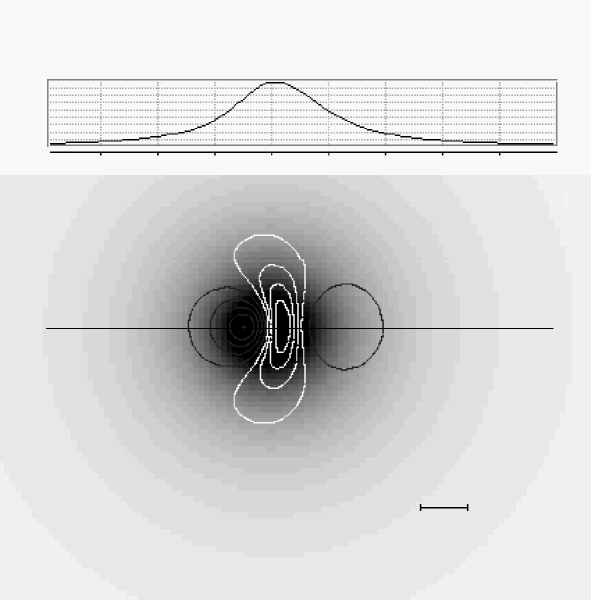
Figure 14: Upper panel: Integrated X–ray profile of the simulated system composed by two subsystems, both following a Beta model profile but with different model parameters (see text). Lower panel: Surface brightness distribution of the simulated system with, superimposed, the contour levels of the Beta model residuals. White (dark/gray) contours represent negative (positive) residuals. As a reference, the size of the fitted core radius is drawn.

  

5.2 Investigating the likely merger cluster

The absence of a macroscopic elongation of the galaxy and ICM distributions and the poor significance of the velocity gradient suggests that the evidence of substructure we detect is a trace of minor/old accretion phenomena or that the direction of the cluster merger is aligned with the LOS. A LOS merger direction would make more difficult the analysis of the cluster internal dynamics. Another example of a cluster merger along the LOS is the galaxy cluster CL 0024+17, an apparently relaxed system, which is actually a collision of two clusters, the interaction occurring along our LOS, as shown by about 300 redshifts in the cluster field (Czoske et al. czo02 (2002) and refs. therein).

The cluster merger scenario is generally consistent with the absence of the cool core. In fact, although simulations yield ambivalent results about the role of mergers in destroying cool cores (Poole et al. poo06 (2006); Burns et al. bur08 (2008)), observations seem to favor cool core destruction through cluster mergers (Allen et al. all01 (2001); Sanderson et al. san06 (2006)). In particular, the LOS merging direction might explain the high compactness of A2294 with respect to other non–cool core clusters (Bauer et al. bau05 (2005), see their Fig. 3). Also notice that our new data on the BCG exclude the presence of H$\alpha$ emission previously reported by Crawford et al. (cra95 (1995)), thus reconducting A2294 to a quite “normal” non–cool core.

In the framework of a cluster merger where the two subclusters are well traced by the luminous galaxies (for the non–collisional part, i.e. dark matter and galaxies) and the residual image (for the collisional part, i.e. the gas), we can also obtain some information about the evolutionary stage of the merger. Assuming that $\beta_{\rm spec}=1$ for each of the two subclusters, from the values of $\sigma_{\rm V}$ we obtain the X–ray temperatures $T_{\rm X}=$7.0 and 2.8 keV. The observed X–ray temperature is thus $\sim 1.4$ times that of the main subcluster. While the observed X–ray temperature of the merging simulated clusters is still not clear at later times (e.g. 2-3 Gyr after the collision, see ZuHone et al. zuh09 (2009) and refs. therein), numerical simulations agree in finding enhancements of the X–ray temperature around the time of the cross core. After a very sharp rise the temperature peaks just during the core-crossing or just after and then declines (Ricker & Sarazin ric01 (2001); Mastropietro & Burkert mas08 (2008)). Since we do not see evidence for a very hot, arc-shaped feature in the cluster center, we assume that the merger is catched after the core-crossing, i.e. in the outgoing phase. For the case of a 1:3 mass ratio, Fig. 8 of Ricker & Sarazin (ric01 (2001)) suggests a time $\lesssim 0.5$ Gyr after the core-crossing.

At this point we have the minimum observation-based information to apply the two-body model (Beers et al. bee82 (1982); Thompson tho82 (1982)) following the methodology outlined for, e.g., Abell 1240 (Barrena et a. bar09 (2009)). This simple model assumes radial orbits for the clumps with no shear or net rotation of the system. According to the boundary conditions usually considered, the clumps are assumed to begin their evolution at time $t_{0}=0$ with a separation $d_{0}=0$, and are now moving apart or coming together for the first time in their history. In the case of a collision, we assume that the time $t_{0}=0$ with separation $d_{0}=0$ is the time of their core crossing and that we are looking at the system a time $t$ after. The values of the relevant parameters for the two–subclusters system are $t\sim 0.5$ Gyr; the relative LOS velocity in the rest–frame, $V_{\rm rf}\sim 2000$ km s^-1; the projected linear distance between the two clumps, $D\sim 0.1$ $h_{70}^{-1}$ Mpc. The last parameter is deduced from the residual image and thus might be an underestimate for the non-collisional component.

Figure 15: System mass vs. projection angle for bound and unbound solutions (thick solid and thick dashed curves, respectively) of the two–body model applied to the low and high velocity subclusters. Labels BI_a and BI_b indicate the bound and incoming, i.e., collapsing solutions (thick solid curve). Label BO indicates the bound outgoing, i.e., expanding solutions (thick solid curve). Label UO indicates the unbound outgoing solutions (thick dashed curve). The horizontal lines give the range of observational values of the mass system with a 50% error. The thin dashed curve separates bound and unbound regions according to the Newtonian criterion (above and below the thin dashed curve, respectively).

The bimodal model solution gives the total system mass $M_{\rm sys}$, i.e. the sum of the masses of the two subclusters, as a function of $\alpha$, where $\alpha$ is the projection angle between the plane of the sky and the line connecting the centers of the two clumps (e.g., Gregory & Thompson gre84 (1984)). Figure 15 compares the bimodal–model solutions with the observed mass of the system $M_{\rm sys}=2.3$ $\times 10^{15}\;h_{70}^{-1}\;M_{\odot}\;$considering a 50% uncertainty band. Among other solutions, we find the bound outgoing solution (BO) with $\alpha\sim 85$, i.e. the cluster merger is occurring largely in the LOS direction, in agreement with our expectations. In the framework of this solution the SE clump, which is the more X–ray luminous and thus likely the more massive, is moving towards SE in the direction of the observer, while the less X–ray luminous and massive NW subcluster is moving towards NW in the opposite direction with respect to the observer. The true spatial distance between the two subclumps is $D_{\rm 3D}\sim$ 1 $h_{70}^{-1}$ Mpc and the real, i.e. deprojected, velocity difference is $V_{\rm rf,3D}\sim 2000$ km s^-1. In this scenario we expect the presence of a gas shock (Bykov et al. byk08 (2008) and refs. therein). We can estimate the Mach number of the shock from ${\cal M}={\rm v}_{\rm s}/c_{\rm s}$, where ${\rm v}_{\rm s}$ is the velocity of the shock and $c_{\rm s}$ in the sound speed in the pre–shock gas (see e.g., Sarazin sar02 (2002) for a review). The value of $c_{\rm s}$ can be obtained from our estimate of $\sigma_{\rm V}\sim 1070$ for the most massive subcluster. For the value of ${\rm v}_{\rm s}$ we use ${\rm v}_{\rm s}\gtrsim V_{\rm rf,3D}=2000$ km s^-1, since after the core crossing the shock velocity is larger than the subcluster velocity (see Fig. 4 of Springel & Farrar spr07 (2007) and Fig. 14 of Mastropietro & Burkert mas08 (2008)). This leads to ${\cal M}$$\gtrsim 2$, in agreement with moderate Mach numbers $2\leq$${\cal M}$$\leq 4$ expected for shocks due to the cluster merging.

  

In conclusion, present observational evidence is consistent with A2294 being a very massive cluster just formed or in the phase of forming through a merger, i.e. similar to most DARC clusters we previously analyzed (e.g. Boschin et al. bos06 (2006); Barrena et al. 2007a ; Girardi et al. gir08 (2008)). The time–scale of a few fractions of Gyr agrees both with the results of other merging clusters showing radio halos/relics (e.g., Markevitch et al. mar02 (2002); Girardi et al. gir08 (2008); Barrena et al. bar09 (2009)) and with theoretical expectations for radio halos (Brunetti et al. bru09 (2009)). Instead the morphology of the A2294 radio halo is somewhat intriguing. In fact, after the subtraction of discrete sources, the radio halo appears someway elongated along the EW direction as shown by Giovannini et al. (gio09 (2009); their Fig. 10 on the left). Previously analyzed clusters of DARC sample showed radio halos no elongated or elongated in the direction of the merger (Abell 697, Girardi et al. gir06 (2006); Abell 520, Girardi et al. gir08 (2008)). This appearent misaligneament with the project merging direction (SE–NW) deserves to be furtherly investigated.

More in general, to verify our hypothesis about a cluster merger in A2294 and better quantify the merging framework we suggest both the acquisition of many more redshifts in the cluster field and/or deeper X–ray observations. In particular, X–ray data would allow to check the temporal phase of the merger although the LOS geometry of the merger would make difficult the direct observation of the shock (e.g., Markevitch et al. mar05 (2005)). The acquisition of more redshifts might allow to better determine the non-collisional components of the merging subclusters.

- (1) Abell, G. O., Corwin, H. G. Jr., & Olowin, R. P. 1989, ApJS, 70, 1
- (2) Allen, S. W., Ettori, S., & Fabian, A. C. 2001, MNRAS, 324, 877
- (3) Ashman, K. M., Bird, C. M., & Zepf, S. E. 1994, AJ, 108, 2348
- (4) Bardelli, S., Zucca, E., Vettolani, G., et al. 1994, MNRAS, 267, 665
- (5) Barrena, R., Boschin, W., Girardi, M., & Spolaor, M. 2007a, A&A, 467, 37
- (6) Barrena, R., Boschin, W., Girardi, M., & Spolaor, M. 2007b, A&A, 469, 861
- (7) Barrena, R., Girardi, M., Boschin, & Dasí, M. 2009, A&A, 503, 357
- (8) Bauer, F. E., Fabian, A. C., Sanders, J. S., Allen, S. W., & Johnstone, R. M. 2005, MNRAS, 359, 1481
- (9) Beers, T. C., Flynn, K., & Gebhardt, K. 1990, AJ, 100, 32
- (10) Beers, T. C., Forman, W., Huchra, J. P., Jones, C., & Gebhardt, K. 1991, AJ, 102, 1581
- (11) Beers, T. C., Gebhardt, K., Huchra, J. P., et al. 1992, ApJ, 400, 410
- (12) Beers, T. C., Geller, M. J., & Huchra, J. P. 1982, ApJ, 257, 23
- (13) Bertin, E., & Arnouts, S. 1996, A&AS, 117, 393
- (14) Biviano, A., Durret, F., Gerbal, D. et al. 1996, A&A, 311, 95
- (15) Biviano, A., Girardi, M., Giuricin, G., Mardirossian, F., & Mezzetti, M. 1992, ApJ, 396, 35
- (16) Biviano, A., Katgert, P., Mazure, A. et al. 1997, A&A, 321, 84
- (17) Boschin, W., Barrena, R., Girardi, M., & Spolaor, M. 2008, A&A, 487, 33
- (18) Boschin, W., Girardi, M., Barrena, R., et al. 2004, A&A, 416, 839
- (19) Boschin, W., Girardi, M., Spolaor, M., & Barrena, R. 2006, A&A, 449, 461
- (20) Brunetti, G., Cassano, R., Dolag, K., & Setti, G. 2009, A&A, 507, 661
- (21) Buote, D. A. 2002, in “Merging Processes in Galaxy Clusters”, eds. L. Feretti, I. M. Gioia, & G. Giovannini (The Netherlands, Kluwer Ac. Pub.): Optical Analysis of Cluster Mergers
- (22) Buote, D. A., Humphrey, P. J., & Stocke, T. 2005, ApJ, 630, 750
- (23) Burns, J. O., Hallman, E. J., Gantner, B., Motl, P. M., & Norman, M. L. 2008, ApJ, 675, 1125
- (24) Burstein, D., & Heiles, C. 1982, AJ, 87, 1165
- (25) Bykov, A. M., Dolag, K., & Durret, F. 2008, Space Science Reviews, Volume 134, Issue 1-4, pp. 119-140
- (26) Carlberg, R. G., Yee, H. K. C., & Ellingson, E. 1997, ApJ, 478, 462
- (27) Cash, W. 1979, ApJ, 228, 939
- (28) Cassano, R., & Brunetti, G. 2005, MNRAS, 357, 1313
- (29) Cassano, R., & Brunetti, G., Röttgering, H. J. A., & Brüggen, M. 2009, A&A, in press (preprint arXiv:0910.2025v1)
- (30) Cavaliere, A. & Fusco–Femiano, R. 1976, A&A, 49, 137
- (31) Cousins, A. W. J., 1976, Mem. R. Astr. Soc, 81, 25
- (32) Crawford, C. S., Edge, A. C., Fabian, A. C., et al. 1995, MNRAS, 274, 75
- (33) Croston, J. H., Pratt, G. W., Böhringer, et al. 2008, A&A, 431, 443
- (34) Czoske, O., Moore, B., Kneib, J.–P., & Soucail, G. 2002, A&A, 386, 31
- (35) Danese, L., De Zotti, C., & di Tullio, G. 1980, A&A, 82, 322
- (36) Dickey, J. M., & Lockman, F. J. 1990, ARA&A, 28, 215
- (37) Dressler, A., & Shectman, S. A. 1988, AJ, 95, 985
- (38) Ebeling, H., Edge, A. C., Böhringer, H., et al. 1998, MNRAS, 301, 881
- (39) Edwards, L. O. V., Hudson, M. J., Balogh, M. L., & Smith, R. J. 2007, MNRAS, 379, 100
- (40) Ellingson, E., & Yee, H. K. C. 1994, ApJS, 92, 33
- (41) Ensslin, T. A., Biermann, P. L., Klein, U., & Kohle, S. 1998, A&A, 332, 395
- (42) Ensslin, T. A., & Gopal–Krishna 2001, A&A, 366, 26
- (43) Fadda, D., Girardi, M., Giuricin, G., Mardirossian, F., & Mezzetti, M. 1996, ApJ, 473, 670
- (44) Feretti, L. 1999, MPE Report No. 271
- (45) Feretti, L. 2002a, The Universe at Low Radio Frequencies, Proceedings of IAU Symposium 199, held 30 Nov – 4 Dec 1999, Pune, India. Edited by A. Pramesh Rao, G. Swarup, and Gopal–Krishna, 2002., p.133
- (46) Feretti, L. 2005, X–Ray and Radio Connections (eds. L. O. Sjouwerman and K. K. Dyer). Published electronically by NRAO, http://www.aoc.nrao.edu/events/xraydio. Held 3–6 February 2004 in Santa Fe, New Mexico, USA
- (47) Feretti, L. 2006, Proceedings of the XLIst Rencontres de Moriond, XXVIth Astrophysics Moriond Meeting: ”From dark halos to light”, L.Tresse, S. Maurogordato and J. Tran Thanh Van, Eds, e–print astro–ph/0612185
- (48) Feretti, L. 2008, Mem. SAIt, 79, 176
- (49) Feretti, L., Gioia I. M., and Giovannini G. eds., 2002b, Astrophysics and Space Science Library, vol. 272, “Merging Processes in Galaxy Clusters”, Kluwer Academic Publisher, The Netherlands
- (50) Ferrari, C., Govoni, F., Schindler, S., Bykov, A. M., & Rephaeli, Y. 2008, Space Sci. Rev., 134, 93
- (51) Fusco–Femiano, R., & Menci, N. 1998, ApJ, 498, 95
- (52) Giovannini, G., Bonafede, A., Feretti, L., et al. 2009, A&A, 507, 1257
- (53) Giovannini, G., & Feretti, L. 2002, in “Merging Processes in Galaxy Clusters”, eds. L. Feretti, I. M. Gioia, & G. Giovannini (The Netherlands, Kluwer Ac. Pub.): Diffuse Radio Sources and Cluster Mergers
- (54) Giovannini, G., Tordi, M., & Feretti, L. 1999, New Astronomy, 4, 141
- (55) Girardi, M., Barrena, R., & Boschin, W. 2007, Contribution to “Tracing Cosmic Evolution with Clusters of Galaxies: Six Years Later” conference – http://www.si.inaf.it/sesto2007/contributions/Girardi.pdf
- (56) Girardi, M., Barrena, R., Boschin, W., & Ellingson, E. 2008, A&A, 491, 379
- (57) Girardi, M., & Biviano, A. 2002, in “Merging Processes in Galaxy Clusters”, eds. L. Feretti, I. M. Gioia, & G. Giovannini (The Netherlands, Kluwer Ac. Pub.): Optical Analysis of Cluster Mergers
- (58) Girardi, M., Boschin, W., & Barrena, R. 2006, A&A, 455, 45
- (59) Girardi, M., Fadda, D., Giuricin, G. et al. 1996, ApJ, 457, 61
- (60) Girardi, M., Giuricin, G., Mardirossian, F., Mezzetti, M., & Boschin, W. 1998, ApJ, 505, 74
- (61) Girardi, M., & Mezzetti, M. 2001, ApJ, 548, 79
- (62) Goto, T. 2005, MNRAS, 359, 141
- (63) González–Casado, G., Mamon, G. A., & Salvador–Solé, E. 1994, ApJ, 433, 61
- (64) Gregory, S. A., & Thompson, L. A. 1984, ApJ, 286, 422
- (65) Gullixson, C. A. 1992, in “Astronomical CCD Observing and Reduction techniques” (ed. S. B. Howell), ASP Conf. Ser., 23, 130
- (66) Hart, B. 2008, PhDT, arXiv e–print 0801.4093
- (67) Hashimoto, Y., Böhringer, H., Henry, J. P., Hasinger, G., & Szokoly, G. 2007, A&A, 467, 485
- (68) Hoeft, M., Brüggen, M., & Yepes, G. 2004, MNRAS, 347, 389
- (69) Johnson, H. L., & Morgan, W. W. 1953, ApJ, 117, 313
- (70) Jones, C., & Forman, W. 1999, ApJ, 511, 65
- (71) Kempner, J. C., Blanton, E. L., Clarke, T. E. et al. 2004, Proceedings of the conference “The Riddle of Cooling Flows in Galaxies and Clusters of Galaxies”, eds. T. H. Reiprich, J. C. Kempner, & N. Soker, e–print arXiv astro–ph/0310263
- (72) Kennicutt, R. C. 1992, ApJS, 79, 225
- (73) Landolt, A. U. 1992, AJ, 104, 340
- (74) Leccardi, A., & Molendi, S. 2008, A&A, 486, 359
- (75) Limber, D. N., & Mathews, W. G. 1960, ApJ, 132, 286
- (76) López–Cruz, O., Barkhouse, W. A., & Yee, H. K. C. 2004, ApJ, 614, 679
- (77) Malumuth, E. M., Kriss, G. A., Dixon, W. Van Dyke, Ferguson, H. C., & Ritchie, C. 1992, AJ, 104, 495
- (78) Markevitch, M., Gonzalez, A. H., David, L., et al. 2002, ApJ, 567, 27
- (79) Markevitch, M., Govoni, F., Brunetti, G, & Jerius, D. 2005, ApJ, 627, 733
- (80) Mastropietro, C., & Burkert, A. 2008, MNRAS, 389, 967
- (81) Maughan, B. J., Jones, C., Forman, W., & Van Speybroeck, L. 2008, ApJS, 174, 117
- (82) Merritt, D. 1988, in “The Minneosota lectures on clusters of galaxies and large–scale structure” (A90–36758 15–90). San Francisco, CA, Astronomical Society of the Pacific, 1988, p. 175–196.
- (83) Menci, N., & Fusco–Femiano, R. 1996, ApJ, 472, 46
- (84) Mushotzky, R. F., & Scharf, C. A. 1997, ApJ, 482, L13
- (85) NAG Fortran Workstation Handbook, 1986 (Downers Grove, IL: Numerical Algorithms Group)
- (86) Neumann, D. M., & Arnaud, M. 1999, A&A, 348, 711
- (87) Neumann, D. M., & Arnaud, M. 2005, A&A, 439, 465
- (88) Ota, N., Pointecouteau, E.; Hattori, M.; & Mitsuda, K. 2004, ApJ, 601, 1200
- (89) Owen, F., Morrison, G., & Voges, W. 1999, proceedings of the workshop “Diffuse Thermal and Relativistic Plasma in Galaxy Clusters”, eds. H. Böhringer, L. Feretti, & P. Schuecker, MPE Report 271, pp. 9–11
- (90) Peres, C. B, Fabian, A. C., Edge, A. C., et al. 1998, MNRAS, 298, 416
- (91) Pisani, A. 1993, MNRAS, 265, 706
- (92) Pisani, A. 1996, MNRAS, 278, 697
- (93) Poggianti, B. M. 1997, A&AS, 122, 399
- (94) Poole, G. B., Fardal, M. A., Babul, A., et al. 2006, MNRAS, 373, 881
- (95) Press, W. H., Teukolsky, S. A., Vetterling, W. T., & Flannery, B. P. 1992, in Numerical Recipes (Second Edition), (Cambridge University Press)
- (96) Quintana, H., Carrasco, E. R., & Reisenegger, A. 2000, AJ, 120, 511
- (97) Raymond, J. C., & Smith, B. W. 1977, ApJS, 35, 419
- (98) Ricker, P. M., & Sarazin, C. L. 2001, ApJ, 561, 621
- (99) Rizza, E., Burns, J. O., Ledlow, M. J. et al. 1998, MNRAS, 301, 328
- (100) Rizza, E., Morrison, G. E., Owen, F. N., et al. 2003, AJ, 126, 119
- (101) Roettiger, K., Burns, J. O., & Loken, C. 1996, ApJ, 473, 651
- (102) Roettiger, K., Burns, J. O., & Stone, J. M. 1999, ApJ, 518, 603
- (103) Roettiger, K., Loken, C., & Burns, J. O. 1997, ApJS, 109, 307
- (104) Sanderson, A. J. R., Ponman, T. J., & O’Sullivan, E. 2006, MNRAS, 372, 1496
- (105) Sarazin, C. L. 2002, in “Merging Processes in Galaxy Clusters”, eds. L. Feretti, I. M. Gioia, & G. Giovannini (The Netherlands, Kluwer Ac. Pub.): The Physics of Cluster Mergers
- (106) Springel, V., & Farrar, G. R. 2007, MNRAS, 380, 911
- (107) The, L. S., & White, S. D. M. 1986, AJ, 92, 1248
- (108) Thompson, L. A. 1982, in IAU Symposium 104, Early Evolution of the Universe and the Present Structure, eds. G.O. Abell and G. Chincarini (Dordrecht: Reidel)
- (109) Tonry, J., & Davis, M. 1979, ApJ, 84, 1511
- (110) Tribble, P. C. 1993, MNRAS, 261, 57
- (111) Vikhlinin, A., Forman, W., & Jones, C. 1999, ApJ, 525, 47
- (112) Wainer, H., & Schacht, S. 1978, Psychometrika, 43, 203
- (113) ZuHone, J. A., Ricker, P. M., Lamb, D. Q., & Karen Yang, H.–Y. 2009, ApJ, 699, 1004