Static Properties of Polymer Melts in Two Dimensions

Abstract

Self-avoiding polymers in strictly two-dimensional ($d=2$) melts are investigated by means of molecular dynamics simulation of a standard bead-spring model with chain lengths ranging up to $N=2048$. The chains adopt compact configurations of typical size $R(N)\sim N^{\nu}$ with $\nu=1/d$. The precise measurement of various distributions of internal chain distances allows a direct test of the contact exponents $\Theta_{0}=3/8$, $\Theta_{1}=1/2$ and $\Theta_{2}=3/4$ predicted by Duplantier. Due to the segregation of the chains the ratio of end-to-end distance $R_{\text{e}}(N)$ and gyration radius $R_{\text{g}}(N)$ becomes $R_{\text{e}}^{2}(N)/R_{\text{g}}^{2}(N)\approx 5.3<6$ for $N\gg 100$ and the chains are more spherical than Gaussian phantom chains. The second Legendre polynomial $P_{2}(s)$ of the bond vectors decays as $P_{2}(s)\sim 1/s^{1+\nu\Theta_{2}}$ measuring thus the return probability of the chain after $s$ steps. The irregular chain contours are shown to be characterized by a perimeter length $L(N)\sim R(N)^{d_{\mathrm{p}}}$ of fractal line dimension $d_{\mathrm{p}}=d-\Theta_{2}=5/4$. In agreement with the generalized Porod scattering of compact objects with fractal contour the Kratky representation of the intramolecular structure factor $F(q)$ reveals a strong non-monotonous behavior with $q^{d}F(q)\sim 1/(qR(N))^{\Theta_{2}}$ in the intermediate regime of the wave vector $q$. This may allow to confirm the predicted contour fractality in a real experiment.

I Introduction

Dense self-avoiding polymers in two dimensions (2D) have been considered theoretically de Gennes (1979); Duplantier (1989); Semenov and Johner (2003); Jakobson et al. (2003), by means of computer simulation Baumgärtner (1982); Carmesin and Kremer (1990); Ostrovsky et al. (1997); Nelson et al. (1997); Polanowski and Pakula (2002); Balabaev et al. (2002); Yethiraj (2003); Yethiraj et al. (2005); Cavallo et al. (2003); Cavallo et al. (2005a, b); Meyer et al. (2009) and more recently even in real experiments Maier and Rädler (1999); Wang and Foltz (2004); Gavranovic et al. (2005); Sun et al. (2007); Zhao and Granick (2007); Srivastava and Basu (2009). It is now generally accepted Duplantier (1989); Semenov and Johner (2003); Jakobson et al. (2003); Baumgärtner (1982); Carmesin and Kremer (1990); Nelson et al. (1997); Polanowski and Pakula (2002); Balabaev et al. (2002); Yethiraj (2003); Cavallo et al. (2005a); Maier and Rädler (1999); Sun et al. (2007); Meyer et al. (2009) (with the notable exception of Refs. Ostrovsky et al. (1997) and Wang and Foltz (2004)) that these chains adopt compact and segregated conformations at high densities, i.e. as first suggested by de Gennes de Gennes (1979) the typical chain size $R(N)$ scales as

$$N\approx\rho R^{d}(N)$$ (1)

with $N$ being the chain length, $\rho$ the monomer number density and $d=2$ the spatial dimension. We assume here that monomer overlap and chain intersections are strictly forbidden Semenov and Johner (2003). Compactness and segregation are expected to apply not only on the scale of the total chain of $N$ monomers but also to subchains comprising $s$ monomers Semenov and Johner (2003); Sun et al. (2007), at least as long as $s$ is not too small. The typical size $R(s)$ of subchains should thus scale as

$$R(s)\approx(s/\rho)^{\nu}\mbox{ for }1\ll s\leq N$$ (2)

with a Flory exponent $\nu=1/d=1/2$ set by the spatial dimension. Interestingly, the direct visualization of chain conformations is possible for DNA molecules Maier and Rädler (1999, 2000, 2001), nanorope polymer chains Wang and Foltz (2004) or brushlike polymers Sun et al. (2007) adsorbed on strongly attractive surfaces or confined in thin films by means of fluorescence microscopy Maier and Rädler (1999, 2000) or atomic force microscopy Wang and Foltz (2004); Sun et al. (2007). The experimental verification of the various conformational properties discussed in this paper, such the one described by Eq. (2), is thus conceivable for these systems Sun et al. (2007).

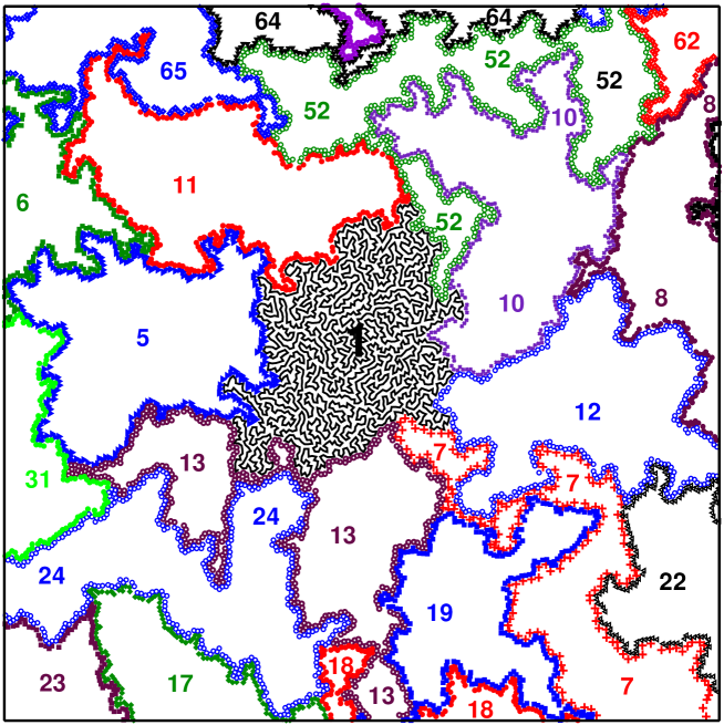
Figure 1: Snapshot of a 2D polymer melt with chain length $N=2048$ and monomer number density $\rho=7/8$. Due to the excluded volume interactions the monomers do barely overlap and chain intersections are strictly forbidden. One chain in the middle is fully drawn while for the other chains only the perimeter monomers interacting with other chains are indicated. A perimeter monomer is defined here as having at least one monomer not belonging to the same chain within a distance $r\leq a=1.2$. Numbers refer to an arbitrary chain index used for computational purposes. The chains are compact, i.e., they fill space densely, and interact typically with about $6$ other chains. However, compactness does apparently not imply a disk-like shape which would minimize the perimeter length $L(N)$. Quantitative analysis reveals that the contours are fractal with a fractal line dimension $d_{\mathrm{p}}=5/4$.

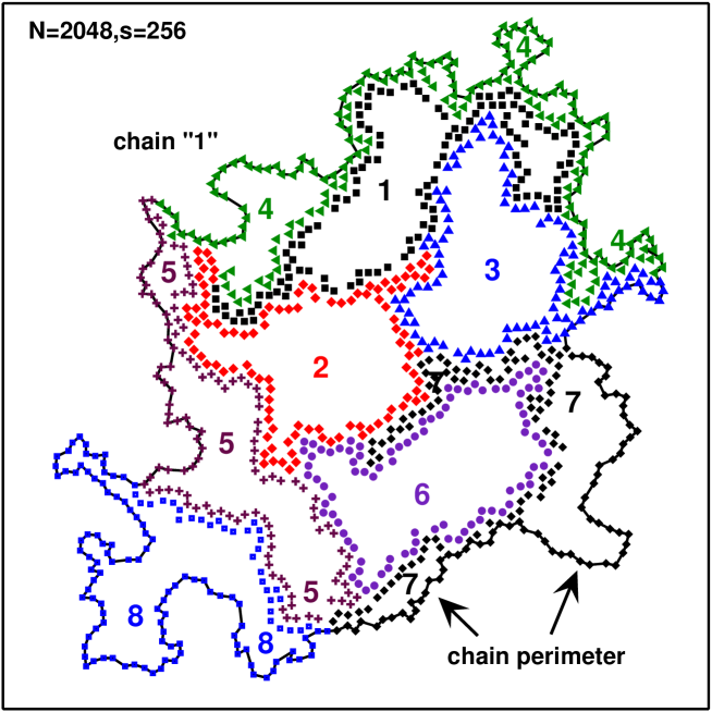
Figure 2: Self-similarity of compactness and perimeter fractality on all scales shown for the chain “1” from the snapshot Fig. 1. The solid line indicates the perimeter of this chain with respect to monomers of other chains. We consider 8 consecutive subchains of length $s=256$ and compute their respective perimeter monomers being close to monomers from other chains or subchains. The subchains are compact and of irregular shape, just as the total chains ($s=N$) presented in Fig. 1.

Compactness does obviously not imply Gaussian chain statistics de Gennes (1979) (as incorrectly stated, e.g., in Wang and Foltz (2004)) nor does segregation of chains and subchains impose disk-like shapes minimizing the average perimeter length $L(s)$ of chains and subchains Semenov and Johner (2003). The contour boundaries are in fact found to be highly irregular as is revealed by the snapshots presented in Fig. 1 and Fig. 2. Elaborating a short communication made recently Meyer et al. (2009) we present here theoretical arguments and molecular dynamics simulations demonstrating that the contours are in fact fractal, scaling as

$$L(s)\sim R(s)^{d_{\mathrm{p}}}\sim s^{1-\nu\Theta_{2}},$$ (3)

with $d_{\mathrm{p}}=d-\Theta_{2}=5/4>1$ being the fractal line dimension Mandelbrot (1982). Our work is based on the pioneering work by Duplantier who predicted a contact exponent $\Theta_{2}=3/4$ Duplantier (1989) and a more recent paper by Semenov and one of us (A.J.) Semenov and Johner (2003). In contrast to many other possibilities to characterize numerically the compact chain conformations the perimeter length is of interest since it can be related to the intrachain structure factor $F(q)$ with $\mathbf{q}$ being the wave vector. It is thus accessible experimentally, at least in principle, by means of small-angle neutron scattering experiments to all polymers which can be appropriately labeled Higgins and Benoît (1996). Specifically, it will be demonstrated that due to the generalized Porod scattering of compact objects Higgins and Benoît (1996); Bale and Schmidt (1984); Wong and Bray (1988) the structure factor of dense 2D polymers should scale in the intermediate wave vector regime as

$$F(q)\approx N/(qR(N))^{d+\Theta_{2}}\sim N^{-3/8}q^{-11/4}$$ (4)

for sufficiently long chains and not as $F(q)\sim N^{0}q^{-2}$ as numerous authors have assumed Carmesin and Kremer (1990); Maier and Rädler (1999); Polanowski and Pakula (2002); Yethiraj (2003).

The present paper is organized as follows. In Sec. II we recall the computational model used for this study. Our mainly numerical results are presented in Sec. III. We confirm first the compactness of the chain conformations by considering the typical size of chains and subchains (Sec. III.1). Corrections to this leading power-law behavior due to chain-end effects caused by the confinement of the chains will be analyzed in Sec. III.3. That $\nu=1/2$ does not imply Gaussian chain statistics will be emphasized by the scaling analysis of various intrachain properties such as the histograms of inner chain distances $G_{i}(r)$ in Sec. III.2, the bond-bond correlation functions $P_{1}(s)$ and $P_{2}(s)$ in Sec. III.4 or the single chain structure factor $F(q)$ in Sec. III.7. Two (related) scaling arguments will be given in Sec. III.6 and at the end of Sec. III.7, demonstrating the scaling of the perimeter length $L(s)$, Eq. (3). The analytic calculation of the structure factor $F(q)$ for 2D melts is relegated to the Appendix. A discussion of possible consequences of the observed static properties for the dynamics of dense 2D solutions and melts concludes the paper in Sec. IV.

II Computational details

Our numerical results are obtained by standard molecular dynamics simulations of monodisperse linear chains at high densities. The coarse-grained polymer model Hamiltonian is essentially identical to the standard Kremer-Grest (KG) bead-spring model Grest and Kremer (1986); Kremer and Grest (1990) which has been used in numerous simulation studies of diverse problems in polymer physics Grest and Kremer (1986); Kremer and Grest (1990); Dünweg (1993); Attig et al. (2004). The non-bonded excluded volume interactions are represented by a purely repulsive Lennard-Jones potential Frenkel and Smit (2002)

$$U_{\text{nb}}(r)=4\epsilon\left[(\sigma/r)^{12}-(\sigma/r)^{6}\right]+\epsilon\mbox{ for }r/\sigma\leq 2^{1/6}$$ (5)

and $U_{\text{nb}}(r)=0$ elsewhere. The Lennard-Jones potential does not act between adjacent monomers of a chain which are topologically connected by a simple harmonic spring potential

$$U_{\text{b}}(r)=k_{\text{b}}(r-l_{\text{b}})^{2}$$ (6)

with a spring constant $k_{\text{b}}=338\epsilon$ and a bond reference length $l_{\text{b}}=0.967\sigma$. Both constants have been calibrated to the “finite extendible nonlinear elastic” (FENE) springs of the original KG model. Lennard-Jones units are used throughout this paper ($\epsilon=\sigma=1$). The classical equations of motion of the multichain system are solved via the Velocity-Verlet algorithm at constant temperature using a Langevin thermostat with friction constant $\gamma=0.5$ Frenkel and Smit (2002).

We focus in this presentation on melts of density $\rho=7/8=0.875$ at temperature $T=1$. Due to the excluded volume potential monomer overlap is strongly reduced as may be seen from the pair correlation function $g(r)$ shown in Fig. 3. The bonding potential, Eq. (6), prevents the long range correlations which would otherwise occur at such a high density for a 2D system of monodisperse Lennard-Jones beads Chaikin and Lubensky (1995); Frenkel and Smit (2002). As shown in the inset of Fig. 3 we have in fact a dense liquid and the oscillations of $g(r)-1$ decay rapidly with an exponential cut-off. The parameters of the model Hamiltonian and the chosen density and temperature makes chain intersections impossible, as can be seen from the snapshot of “chain 1” presented in Fig. 1. We simulate thus “self-avoiding walks” in the sense of the first model class discussed in Ref. Semenov and Johner (2003).

Monodisperse systems with chain lengths $N$ ranging between $N=32$ up to $N=2048$ have been sampled using periodic square boxes containing either $98304$ or $196608$ monomers. The larger box of linear length $474.02$ corresponds to $96$ chains of length $N=2048$. Some conformational properties discussed below are summarized in the Table. Except the systems with $N=2048$, all chains have diffused over at least 10 times their radius of gyration $R_{\text{g}}(N)$ providing thus sufficiently good statistics. Note that our largest chain is about an order of magnitude larger than the largest chains used in previous computational studies of dense 2D melts: $N=59$ by Baumgärtner in 1982 Baumgärtner (1982), $N=100$ by Carmesin and Kremer in their seminal work in 1990 Carmesin and Kremer (1990), $N=100$ by Nelson et al. in 1997 Nelson et al. (1997), $N=32$ by Polanowski and Pakula in 2002 Polanowski and Pakula (2002), $N=60$ by Balabaev et al. in 2002 Balabaev et al. (2002), $N=256$ by Yethiraj in 2003 Yethiraj (2003) and $N=256$ by Cavallo et al. in 2005 Cavallo et al. (2005a, b). The presented data was obtained on IBM power 6 with the LAMMPS Version 21May2008 Plimpton (1995). It is part of a broader study where we have systematically varied density, system size and friction coefficient to confirm the robustness of theory and simulation with respect to these parameters. Since the chain length is computationally the limiting factor fixing the number of “blobs” de Gennes (1979) at a given density we present data at the largest density, i.e. the largest number of blobs, where we have been able to equilibrate chains of $N=2048$.

III Numerical results

III.1 Chain and subchain size: Compactness

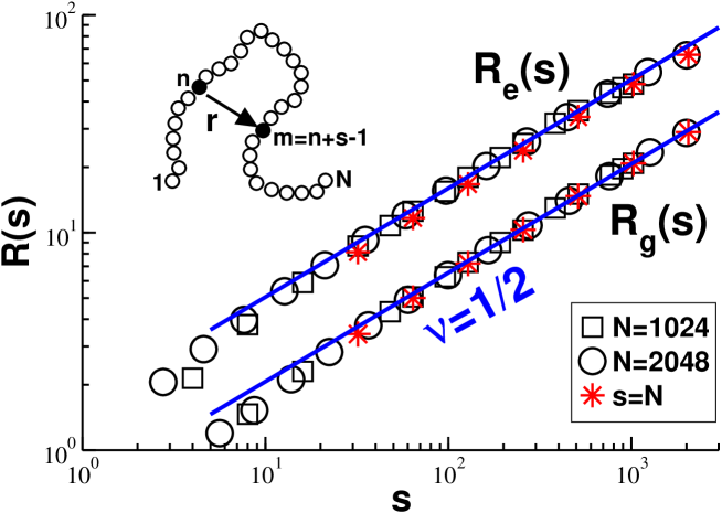
Figure 4: End-to-end distance $R_{\text{e}}(s)=\langle\mathbf{r}^{2}\rangle^{1/2}$ (top data) and radius of gyration $R_{\text{g}}(s)$ (bottom data) of “subchains” or “chain segments” Wittmer et al. (2007) containing $s=m-n+1$ monomers as indicated by the sketch on the left hand side. The data is averaged over all $s$-subchains possible in a chain of length $N$. Open symbols refer to subchains with $s\leq N$ for $N=1024$ (squares) and $N=2048$ (spheres), stars to overall chain properties ($s=N$). The indicated power-law slopes confirm Eq. (2), i.e. the chains are compact on all scales.

Figure 4 confirms that 2D chains are indeed compact as stated in Eq. (1) and Eq. (2) and as shown in Fig. 1 for chains and in Fig. 2 for subchains of arc-length $s$. The typical size $R(s)$ of subchains is characterized by either the root-mean-square end-to-end distance $R_{\text{e}}(s)$ or the radius of gyration $R_{\text{g}}(s)$ Doi and Edwards (1986); Wittmer et al. (2007). As indicated in the sketch we consider a subchain between two monomers $n$ and $m=n+s-1$ and average over all pairs $(n,m)$ possible in a chain of length $N$ following Wittmer et al. (2004); Auhl et al. (2003); Wittmer et al. (2007). Averaging only over subchains at the curvilinear chain center ($n,m\approx N/2$) slightly reduces chain end effects, however the difference is negligible for the larger chains, $N\geq 1024$, we focus on. The limit $s=N$ corresponds obviously to the standard end-to-end vector $R_{\text{e}}(N)$ and gyration radius $R_{\text{g}}(N)$ of the total chain. Open symbols refer to subchains of length $s\leq N$ with $N=1024$ (squares) and $N=2048$ (spheres), stars to total chain properties ($s=N$). In agreement with various numerical Baumgärtner (1982); Carmesin and Kremer (1990); Nelson et al. (1997); Polanowski and Pakula (2002); Balabaev et al. (2002); Yethiraj (2003); Cavallo et al. (2005a) and experimental studies Maier and Rädler (1999); Sun et al. (2007) the presented data confirms that the chains are compact, i.e. $\nu=1/d$ (thin lines), and this on all length scales with $1\ll s\leq N$.

The segregation of the chains may also be shown by computing the average number $n_{\text{chain}}$ of chains in contact with a reference chain, i.e. having at least one monomer closer than a distance $a\approx 2$ to a monomer of the reference chain (Sec. III.6). Depending weakly on $a$, we find $n_{\text{chain}}\approx 6$, as one may expect for 2D colloids and in agreement with Fig. 1. At variance to any open non-segregated polymer-like structure $n_{\text{chain}}$ does thus not increase with chain length $N$. An alternative way to confirm this statement is to count the centers of mass around the reference chain’s center of mass by integrating the center-of-mass pair-correlation function $g_{\text{cm}}(r)$, a structureless function without oscillations (not shown). One verifies that 6 chains are found in a shell of about $2R_{\text{g}}(N)$ and this irrespective of $N$.

III.2 Segment size distributions and contact exponents

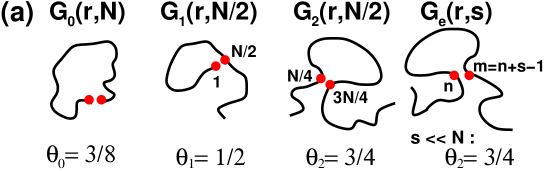
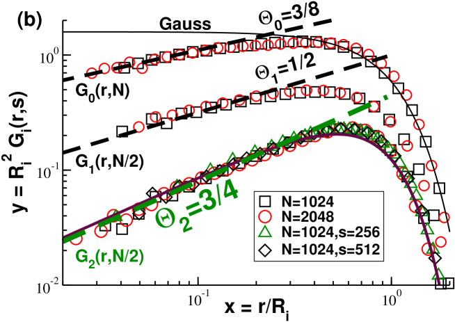
Figure 5: (a) Sketch of the intrachain probability distributions $G_{i}(r,s)$ described in the main text and the contact exponents $\Theta_{i}$ predicted by Duplantier Duplantier (1989). (b) Scaling plots are presented for $G_{0}(r,N)$, $G_{1}(r,N/2)$ and $G_{2}(r,N/2)$ for $N=1024$ (squares) and $N=2048$ (spheres) and for $G_{\text{e}}(r,s)$ for $N=1024\gg s$ with $s=256$ (triangles) and $s=512$ (diamonds). All data for different $N$ and $s$ collapse on the respective universal master curves if $y=R_{i}^{2}G_{i}(r,s)$ is plotted vs. the reduced distance $x=r/R_{i}$ with $R_{i}^{2}$ being the second moment of the corresponding distribution. The thin line indicates the Gaussian distribution $y=\exp(-x^{2})/\pi$ expected for ideal chains in 2D. The power laws $y\approx x^{\Theta_{i}}$ observed for $x\ll 1$ (dashed lines) confirm Duplantier’s prediction. The solid line at the bottom shows the Redner-des Cloizeaux formula, Eq. (8), for $G_{2}(r,s=N/2)\approx G_{\text{e}}(r,s)$.

Being characterized by the same Flory exponent $\nu$ as their three dimensional (3D) counterparts does by no means imply that 2D melts are Gaussian Duplantier (1989); Semenov and Johner (2003). This can be directly seen, e.g., from the different probability distributions of the intrachain vectors $\mathbf{r}=\mathbf{r}_{m}-\mathbf{r}_{n}$ presented in Fig. 5. To simplify the plot we have focused on the two longest chains $N=1024$ and $N=2048$ we have simulated. As illustrated in panel (a),

• $G_{0}(r,s=N)$ characterizes the distribution of the total chain end-to-end vector ($n=1$, $m=N$),

• $G_{1}(r,s=N/2)$ the distance between a chain end and a monomer in the middle of the chain ($n=1$, $m=N/2$),

• $G_{2}(r,s=N/2)$ the distribution of an inner segment vector between the monomers $n=N/4$ and $m=3N/4$,

• while the “segmental size distribution” $G_{\text{e}}(r,s)$ Wittmer et al. (2007) averages over all pairs of monomers $(n,m=n+s-1)$ for $s\leq N$.

The second index $s$ indicated in $G_{i}(r,s)$ characterizes the length of the subchain between the two monomers $n$ and $m$. As shown in panel (b), all data for different $N$ and $s$ collapse on three distinct master curves if the axes are made dimensionless using the second moment $R_{i}^{2}$ of the respective distribution. The only relevant length scale is thus the typical size of the subchain itself. The distributions are all non-monotonous and are thus qualitatively different from the Gaussian (thin line) expected for uncorrelated ideal chains. Confirming Duplantier’s predictions Duplantier (1989) we find

$$R_{i}^{d}G_{i}(r,s)=x^{\Theta_{i}}f_{i}(x)$$ (7)

with $x=r/R_{i}$ being the scaling variable and the contact exponents $\Theta_{0}=3/8$, $\Theta_{1}=1/2$ and $\Theta_{2}=3/4$ (dashed lines) describing the small-$x$ limit where the universal functions $f_{i}(x)$ become constant. Especially the largest of these exponents, $\Theta_{2}$, is clearly visible. The contact probability for two monomers of a chain in a 2D melt is thus strongly suppressed compared to ideal chain statistics ($\Theta_{0}=\Theta_{1}=\Theta_{2}=0$).

The rescaled distributions show exponential cut-offs for large distances. The Redner-des Cloizeaux formula des Cloizeaux and Jannink (1990) is a useful interpolating formula which supposes that

$$f_{i}(x)=c_{i}\exp(-k_{i}x^{2}).$$ (8)

The constants $k_{i}=1+\Theta_{i}/2$ and $c_{i}=k_{i}^{k_{i}}/\pi\Gamma(k_{i})$ with $\Gamma(z)$ being the Gamma function Abramowitz and Stegun (1964) are imposed by the normalization and the second moment of the distributions Everaers et al. (1995). This formula is by no means rigorous but yields reasonable parameter free fits as it is shown by the solid line for $f_{2}(x)$.

Obviously, $G_{\text{e}}(r,s)\approx G_{0}(r,N)$ for very large subchains $s\rightarrow N$ (not shown). As can be seen, the rescaled distributions $G_{\text{e}}(r,s)$ and $G_{2}(r,N/2)$ become identical if $1\ll s\ll N$. It is for this reason that the exponent $\Theta_{2}$ is central for asymptotically long chains as will become obvious below in Sec. III.6 and Sec. III.7. The two exponents $\Theta_{0}$ and $\Theta_{1}$ are only relevant if the measured property specifically highlightes chain end effects as in the example given in the next subsection.

III.3 Chain and subchain size: Corrections to asymptotic scaling

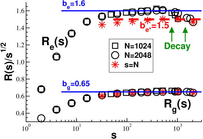
Figure 6: Reduced typical subchain size $R(s)/s^{1/2}$ as characterized by the root-mean-square end-to-end distance $R_{\text{e}}(s)$ (top data) and the radius of gyration $R_{\text{g}}(s)$ (bottom data) using the same symbols as in Fig. 4. Interestingly, $R_{\text{e}}(s)/s^{1/2}$ decays for $s>N/2$ due to chain-end effects. The solid horizontal lines indicate the effective segment sizes $b_{\text{e}}=1.6$ and $b_{\text{g}}=0.65$ obtained for $100\ll s\ll N$ from $R_{\text{e}}(s)/s^{1/2}$ and $R_{\text{g}}(s)/s^{1/2}$, respectively. The dashed line corresponds to an apparent effective segment size $b_{\text{e}\star}=1.5$ from the end-to-end distances $R_{\text{e}}(N)$ of our longest chains.

The log-log representation chosen in Fig. 4 masks deliberately small corrections to the leading power law due to chain end effects which exist in 2D as they do in 3D melts Wittmer et al. (2007). These are revealed in Fig. 6 presenting $R_{\text{e}}(s)/s^{1/2}$ and $R_{\text{g}}(s)/s^{1/2}$ vs. $s$ and $R_{\text{e}}(N)/N^{1/2}$ and $R_{\text{g}}(N)/N^{1/2}$ vs. $N$ using log-linear coordinates and the same symbols as in Fig. 4. The reduced radius of gyration (bottom data) becomes in fact rapidly constant and chain length independent. As emphasized by the bottom horizontal line we find

$$b_{\text{g}}\approx R_{\text{g}}(s)/s^{1/2}\approx R_{\text{g}}(N)/N^{1/2}\mbox{ for }s,N\gg 100$$ (9)

with $b_{\text{g}}=0.65$ for $\rho=7/8$. Interestingly, we observe non-monotonous behavior for $R_{\text{e}}(s)/s^{1/2}$ with a decay for $s>N/2$. Due to this decay $R_{\text{e}}(N)/N^{1/2}$ (stars) is systematically below the corresponding internal chain distance $R_{\text{e}}(s)/s^{1/2}$. If fitted from the chain end-to-end distances one obtains an effective segment size Doi and Edwards (1986)

$$b_{\text{e}\star}\approx R_{\text{e}}(N)/N^{1/2}\approx 1.5\mbox{ for }100\ll N,$$ (10)

as shown by the dashed line. (The index $\star$ indicates that we refer to the total chain.) This value corresponds to the ratio $R_{\text{e}}^{2}(N)/R_{\text{g}}^{2}(N)\approx 5.3<6$ given in the Table. It confirms similar observations made in previous simulations using much shorter chains Baumgärtner (1982); Carmesin and Kremer (1990); Nelson et al. (1997); Yethiraj (2003). If on the other hand the effective segment size $b_{\text{e}}$ is obtained from the internal distances this yields

$$b_{\text{e}}\approx R_{\text{e}}(s)/s^{1/2}\approx 1.6\mbox{ for }100\ll s\ll N,$$ (11)

as indicated by the top solid line. This value is consistent with a ratio $R_{\text{e}}^{2}(s)/R_{\text{g}}^{2}(s)=(b_{\text{e}}/b_{\text{g}})^{2}\approx 6$ as one expects in any dimension due to Doi and Edwards (1986)

$$R_{\text{g}}^{2}(s)=\frac{1}{s^{2}}\int_{0}^{s}ds^{\prime}(s-s^{\prime})R_{\text{e}}^{2}(s^{\prime})=\frac{1}{6}b_{\text{e}}^{2}s$$ (12)

where we have assumed $R_{\text{e}}^{2}(s^{\prime})=b_{\text{e}}^{2}s^{\prime}$ for all $s^{\prime}$ up to $s^{\prime}=s$. Since this assumption breaks down for $s\to N$ (as seen in Fig. 6) Eq. (12) is not in conflict with Eq. (10). Note that the integral over $s^{\prime}$ in Eq. (12) is dominated by subchains with $s^{\prime}\approx s/2$ and that thus large subchains of order $s^{\prime}\approx N$ are less relevant for the gyration radius of the total chain $R_{\text{g}}(s=N)$. Hence, the non-monotonous behavior observed for $R_{\text{e}}(s)$ should be barely detectible for the radius of gyration in agreement with Eq. (9).

That a naive fit of $b_{\text{e}}$ from the total chain end-to-end distance $R_{\text{e}}(N)$ leads to a systematic underestimation of the effective segment size of asymptotically long chains is a well-known fact for 3D melts Wittmer et al. (2007). However, both estimations of $b_{\text{e}}$ merge for 3D melts if sufficiently long chains are computed (as may be seen from Eq. (16) and Fig. 4 of Ref. Wittmer et al. (2007)). Apparently, this is not the case in 2D since if $R_{\text{e}}(s)$ or $R_{\text{e}}^{2}(s)/s$ are plotted as a function of $x=s/N$ a nice scaling collapse of the data is obtained for large $x$ and for $N\geq 256$, i.e.

$$R_{\text{e}}^{2}(s)\approx b_{\text{e}}^{2}s^{2\nu}\tilde{f}(x)\mbox{ with }\tilde{f}(x)=\left\{\begin{array}[]{ll}1&\mbox{ if $x\ll 1$}\\ (b_{\text{e}\star}/b_{\text{e}})^{2}&\mbox{ if $x\to 1$}.\end{array}\right.$$ (13)

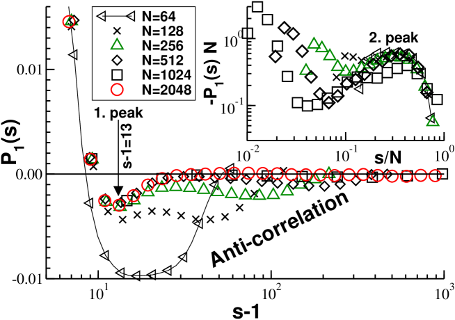
Figure 7: Bond-bond correlation function $P_{1}(s)=\langle\mathbf{e}_{n}\cdot\mathbf{e}_{m}\rangle$ vs. curvilinear distance $s-1$. Main panel: The first Legendre polynomial shows an anti-correlation at $s-1\approx 13$ due to the local wrapping of the chain. Inset: A second anti-correlation peak is visible at $s\approx N/2$ which is caused by the reflection of the confined chain. Due to Eq. (14) this peak is related to the decay of the reduced subchain size $R_{\text{e}}^{2}(s)/s^{1/2}$ visible in Fig. 6.

(Since a very similar scaling plot is presented in the inset of Fig. 7 this figure is not given.) Hence, chain end effects may not scale away with $N\to\infty$ as they do in 3D. A simple qualitative explanation for Eq. (13) is in fact readily given by considering an ideal chain of bond length $b_{\text{e}}$ squeezed into a more or less spherical container of size $R_{c}\sim N^{1/2}$. For $s\ll N$ it is unlikely that the subchain interacts with the container walls and $R_{\text{e}}(s)\approx b_{\text{e}}s^{1/2}$. With $s\to N$ the chain will feel increasingly the confinement reflecting it back from the walls into the center of the container reducing thus the effective segment length $b_{\text{e}\star}$ associated with the chain end-to-end distance. Since the scaling function $\tilde{f}(x)$ must be universal, it should be possible to express the ratio $(b_{\text{e}\star}/b_{\text{e}})^{2}$ — and thus the ratio $R_{\text{e}}^{2}(N)/R_{\text{g}}^{2}(N)=(b_{\text{e}\star}/b_{\text{g}})^{2}$ — in terms of the dimension $d$ and universal compact exponents $\Theta_{0}$, $\Theta_{1}$ and $\Theta_{2}$. The two statistical segment sizes $b_{\text{e}}$ and $b_{\text{e}\star}$ should thus be related. At present we are still lacking a solid theoretical proof for the latter conjection.

III.4 Intrachain orientational correlations

Let $\mathbf{e}_{i}$ denote the normalized tangent vector connecting the monomers $i$ and $i+1$ of a chain. The bond-bond correlation function $P_{1}(s)=\langle\mathbf{e}_{n}\cdot\mathbf{e}_{m}\rangle$ has been shown to be of particular interest for characterizing the deviations from Gaussianity in 3D polymer melts Wittmer et al. (2004, 2007). (As above we average over all pairs of monomers $(n,m)$ with $m=n+s-1$.) The reason for this is that Wittmer et al. (2004)

$$P_{1}(s)\sim-\frac{\partial^{2}R_{\text{e}}^{2}(s)}{\partial s^{2}}$$ (14)

and that thus small deviations from the asymptotic exponent $2\nu=1$ are emphasized Wittmer et al. (2007). $P_{1}(s)$ is presented in Fig. 7 for different chain lengths. Apparently, the bond pairs are aligned only for small arc-lengths with $s<10$. For larger $s$ the bonds are anti-correlated with two characteristic peaks. The first anti-correlation peak visible in panel (a) is due to the local backfolding of the chain contour which can be directly seen from chain 1 drawn in Fig. 1. Note that the chain length dependence disappears for $N>256$. The second anti-correlation peak is shown in panel (b) where $-P_{1}(s)N$ is plotted as function of $x=s/N$. Using Eq. (14) this corresponds exactly to the scaling expected from Eq. (13) with an associated universal function scaling as $-\partial_{x}^{2}(x\tilde{f}(x))$. In agreement with the qualitative explanation mentioned at the end of Sec. III.1, the peak at $s\approx N/2$ can be attributed to the confinement of the chain which causes long segments to be reflected back, i.e. $P_{1}(s)$ must be anti-correlated for large $x$. (Data for $N=2048$ is not presented here due to its insufficient statistics.) We stress finally that altogether this is a rather small effect and essentially $P_{1}(s)\approx\partial^{2}_{s}R_{\text{e}}^{2}(s)\approx 0$ for $s\gg 10^{2}$ and $N\gg 10^{3}$ as already obvious from panel (a). Hence, the first Legendre polynomial confirms that to leading order $2\nu\approx 1$ for sufficiently large chains and segments.

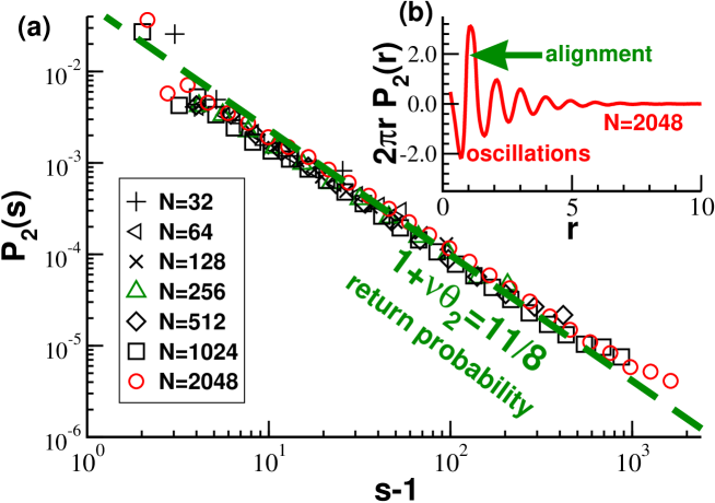
Figure 8: Second Legendre polynomial $P_{2}=\langle\left(\mathbf{e}_{n}\cdot\mathbf{e}_{m}\right)^{2}\rangle-1/2$ as a function of curvilinear distance $s-1$ (a) and as a function of intrachain distance $r$ (b). (a) $P_{2}(s)$ decays over two orders in magnitude as a power law (dashed line) with an exponent $1+\nu\theta_{2}=11/8$ in agreement with a return probability given by Eq. (15). (b) $2\pi rP_{2}(r)$ oscillates strongly with an exponentially decreasing amplitude. Being dominated by a nematic peak at the origin ($r\approx 1$) it acts as a $\delta$-function.

Conceptually more important for the present study is the fact that the second Legendre polynomial $P_{2}(s)=\left<\left(\mathbf{e}_{n}\cdot\mathbf{e}_{m}\right)^{2}\right>-1/2$ given in the main panel of Fig. 8 reveals a clear power law behavior over two orders of magnitude in $s$ (dashed line). This power law is due to (a) the return probability $p_{r}(s)$ after $s$ steps and (b) the “nematic alignment” of two near-by bonds. The alignment of bonds is investigated in the inset of Fig. 8 where the second Legendre polynomial is plotted as a function of the distance $r$ between the mid-points of both bonds. Averages are taken over all intrachain bond pairs with $[r,r+\delta r]$ using a bin of width $\delta r=0.01$. Since $P_{2}(r)$ becomes rapidly chain length independent we only indicate data for $N=2048$. The vertical axis is rescaled with the phase volume $2\pi r$. As can be seen, the orientational correlations oscillate with $r$ and this with a rapidly decaying amplitude. These oscillations are related to the oscillations of the pair correlation function $g(r)$ shown in Fig. 3 and reflect the local packing and wrapping of chains composed of discrete spherical beads. Due to both the oscillations and the decay only bond pairs at $r\approx 1$ matter if we compute $P_{2}(s)$, i.e. if we sum over all distances $r$ at a fixed curvilinear distance $s$. Following Eq. (7) one thus expects

$$P_{2}(s)\approx p_{r}(s)\equiv\lim_{r\rightarrow 0}G_{\text{e}}(r,s)\sim 1/s^{1+\nu\Theta_{2}}=1/s^{11/8}$$ (15)

for $1\ll s\ll N$. The agreement of the data with this power law is excellent and provides, hence, an independent confirmation of the contact exponent $\Theta_{2}=3/4$.

III.5 Chain and subchain shape

As obvious from Fig. 1 and Fig. 2 the conformations of chains and subchains are neither perfectly spherical nor extremely elongated. Having discussed above the chain size we address now the chain shape as characterized by the average aspherity of the gyration tensor. The gyration tensor $\underline{\underline{M}}$ of a subchain between the monomers $n$ and $m=n+s$ is given by

$$M_{\alpha\beta}=\frac{1}{s}\sum_{i=n}^{m}(r_{i,\alpha}-R_{\text{cm},\alpha})(r_{i,\beta}-R_{\text{cm},\beta})$$ (16)

with $R_{\text{cm},\alpha}$ being the $\alpha$-component of the subchains’s center of mass. We remind that the radius of gyration $R_{\text{g}}^{2}(s)$ discussed in Sec. III.1 is given by the trace $\text{tr}(\underline{\underline{M}})=M_{xx}+M_{yy}=\lambda_{1}+\lambda_{2}$ averaged over all subchains and chains with eigenvalues $\lambda_{1}$ and $\lambda_{2}$ obtained from

$$\lambda_{1,2}=\frac{1}{2}\left(\text{tr}(\underline{\underline{M}})\pm\sqrt{\text{tr}(\underline{\underline{M}})^{2}-4\text{det}(\underline{\underline{M}})}\right).$$ (17)

The ratio of the mean eigenvalues $\left<\lambda_{1}\right>/\left<\lambda_{2}\right>$ for $s=N$ is given in the Table. Decreasing slightly with $N$ this “aspect ratio” approaches

$$\left<\lambda_{1}\right>:\left<\lambda_{2}\right>\approx 4.5:1$$ (18)

for our longest chains which corresponds to a reduced principal eigenvalue $\left<\lambda_{1}\right>/R_{\text{g}}^{2}\approx 0.8$. It should be noted that Gaussian chains and dilute good solvent chains in 2D are characterized by an aspect ratio $\left<\lambda_{1}\right>/\left<\lambda_{2}\right>\approx 5.2$ and $6.7$, respectively Bishop and Satiel (1986). Our chains are thus clearly less elongated. The asphericity of the inertia tensor of 2D objects may be further characterized by computing the moments Rudnick and Gaspari (1986); Aronovitz and Nelson (1986); Bishop and Satiel (1986); Maier and Rädler (2001)

$$\Delta_{1}(s)=\frac{\left<\lambda_{1}-\lambda_{2}\right>}{\left<\lambda_{1}+\lambda_{2}\right>}\ ,\ \Delta_{2}(s)=\frac{\left<(\lambda_{1}-\lambda_{2})^{2}\right>}{\left<(\lambda_{1}+\lambda_{2})^{2}\right>}$$ (19)

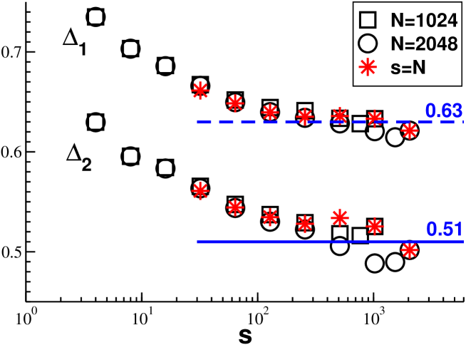
Figure 9: Aspherity of chains (stars) and subchains for $N=1024$ (squares) and $N=2048$ (spheres) using log-linear coordinates. The aspherity is characterized by the moments $\Delta_{1}$ and $\Delta_{2}$ of the eigenvalues $\lambda_{1}$ and $\lambda_{2}$ of the inertia tensor discussed in the main text. Both moments decay weakly with $s$ and $N$. The horizontal lines are guides to the eye indicating possible plateau values for asymptotically long chains.

which are plotted in Fig. 9 for subchains ($s\leq N$) and total chains ($s=N$) using the same symbols as in previous plots. $\Delta_{1}=2\left<\lambda_{1}\right>/R_{\text{g}}^{2}-1$ describes the mean ellipticity and $\Delta_{2}$ the normalized variance of $\lambda_{1}$ and $\lambda_{2}$ Rudnick and Gaspari (1986); Aronovitz and Nelson (1986). Obviously, $\Delta_{1}=\Delta_{2}=1$ for rods and $\Delta_{1}=\Delta_{2}=0$ for spheres. Note that taking the first and the second moments of the ellipticity $(\lambda_{1}-\lambda_{2})/(\lambda_{1}+\lambda_{2})$ of each subchain yields qualitatively similar results (not shown). As one expects, both moments do not depend on whether a chain or a subchain is considered. In agreement with Yethiraj Yethiraj (2003) they decrease weakly with $N$ and $s$. Unfortunately, it is difficult to determine precisely the plateau values one expects for asymptotically large chains and subchains, and the horizontal lines with

$$\Delta_{1}=0.63\mbox{ and }\Delta_{2}=0.51$$ (20)

are merely guides to the eye. Note that Yethiraj Yethiraj (2003) indicates $\Delta_{2}=0.52$ for $N=256$. Considering that the latter value has been obtained at a slightly smaller monomer volume fraction both $\Delta_{2}$-values are compatible. We remind that in two dimensions $\Delta_{1}\approx 0.68$ and $\Delta_{2}=2(d+2)/(5d+4)\approx 0.57$ for Gaussian chains Rudnick and Gaspari (1986); Bishop and Satiel (1986) and $\Delta_{1}\approx 0.74$ and $\Delta_{2}\approx 0.62-0.64$ for dilute good solvent chains according to Refs. Aronovitz and Nelson (1986); Bishop and Satiel (1986); Maier and Rädler (2001); Yethiraj (2003). These values are definitely larger than our respective estimates, Eq. (20), and segregated chains in 2D melts are thus clearly more axisymmetric.

The above analysis has been motivated by recent experimental work on the conformational properties of dilute DNA molecules investigated using fluorescence microscopy Maier and Rädler (2001). A similar characterization of the chain shapes at higher semidilute densities appears therefore feasible, at least in principle.

III.6 The perimeter length

As shown in Fig. 1, 2D chains adopt irregular shapes with perimeters not appearing to be smooth, i.e. characterized by a line dimension $d_{\mathrm{p}}=1$, but clearly fractal ($2>d_{\mathrm{p}}>1$) Mandelbrot (1982). In this subsection we analyze quantitatively this visual impression confirming the announced key result Eq. (3) for the average perimeter length $L(s)$ of chains ($s=N$) and subchains ($s\leq N$).

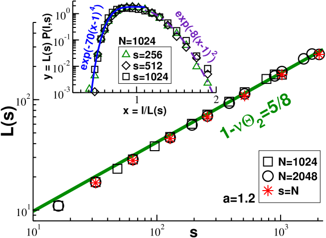
Figure 10: Mean perimeter length $L(s)=\langle l\rangle$ (main panel) and perimeter length distribution $P(l,s)$ (inset) for $a=1.2$. In agreement with Eq. (3) the perimeter scales as $L(s)\sim s^{1-\nu\Theta_{2}}\sim s^{5/8}$ (bold line). Stars refer to perimeters of chains ($s=N$), open symbols to subchains of lengths $s\leq N$ in chains of length $N=1024$ (squares) and $N=2048$ (spheres). The histograms for different $s$ collapse if rescaled using $L(s)$ as presented in the inset for different segment sizes and $N=1024$. The distributions are lopsided decaying much sharper for small-perimeter segments ($l/L(s)\ll 1$). The exponential cut-offs indicated for both limits are phenomenological fits.

We define a perimeter monomer as having at least one monomer not belonging to the same chain or subchain closer than a reference distance $a\approx 1$ essentially set by the monomer density (see below). Specifically, we have used $a=1.2$ in Figs. 1, 2 and 10 and for the data listed in the Table. The number of such perimeter monomers is called $l(s)$, its mean number $L(s)=\left<l(s)\right>$ with $L(s)/s\leq 1$ being the probability that a monomer of a subchain is on its perimeter. (Note that for a continuous chain model a slightly different “box counting” method must be used to obtain a finite perimeter length Mandelbrot (1982).) The main panel of Fig. 10 presents $L(s)$ using the same symbols as in Fig. 4. All data collapses on the same master curve, confirming nicely the announced exponent $1-\nu\Theta_{2}=5/8$ (dashed line) and thus a fractal line dimension $d_{\mathrm{p}}=(5/8)/\nu=5/4$. This result holds provided that chain and subchain lengths are not too small ($N,s\gg 50$).

Having just confirmed Eq. (3) numerically we have still to give a theoretical argument to show where it stems from. Using the return probability $p_{r}(s)\sim 1/s^{1+\nu\Theta_{2}}$ measured in Fig. 8 a simple scaling argument can be given following Semenov and Johner Semenov and Johner (2003). The key point is that a monomer in a long subchain cannot “distinguish” if the contact is realized through the backfolding of its own subchain or by another subchain of length $s$. Since the probability of such a contact, $L(s)/s$, must be proportional to $p_{r}(s)$ times the number $s$ of monomers in the second subchain we have

$$L(s)/s\sim p_{r}(s)\times s\sim s^{-\nu\Theta_{2}}\mbox{ for }1\ll s\leq N$$ (21)

which is identical to Eq. (3). An alternative, but related derivation will be given in Section III.7.

The fluctuations of the perimeter length are characterized in the inset of Fig. 10. We present here the histograms $P(l,s)$ of the number of perimeter monomers for different subchains of lengths $s$ for chains of length $N=1024$. Assuming that the first moment $L(s)$ of the histogram sets the only scale all histograms are successfully brought to a scaling collapse. Please note that the fractality of the perimeter does not imply that the histograms have to be broad. In fact, they decay rather rapidly as indicated by the two phenomenological fits and all moments of the distributions exist. The configurations corresponding to small perimeters are rather strongly suppressed (solid line). At variance to this, the decay for $l(s)-L(s)\gg 0$ is found to be successfully described by a Gaussian (dash-dotted line). The perimeter fluctuations of different contour sections of these configurations are apparently only weakly coupled, if at all.

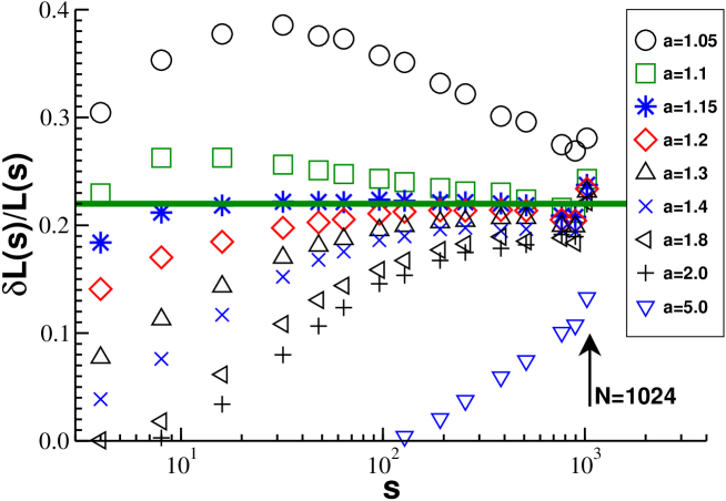
Figure 11: Relative error $\delta L(s)/L(s)$ as a function of $s$ for chains of length $N=1024$ and for different distances $a$ as indicated. The relative error increases for small $s$ and too large $a$-values. It decreases for $a<1.15$ since these values are too small for the given density and not all perimeter monomers are detected. The relative error becomes constant for large $s$ irrespective of the value of $a$. Due to chain end effects the relative error increases slightly for $s\approx N$.

The influence of the distance $a$ used to define a perimeter monomer is investigated in Fig. 11 where we present the “relative error” $\delta L(s)/L(s)\equiv\sqrt{\left<l^{2}\right>/\left<l\right>^{2}-1}$ of the distributions $P(l,s)$. (The relative error for $s=N$ is listed in the Table.) For clarity, only data for one chain length $N=1024$ is given for several $a$ as indicated in the figure. Obviously, if $a$ is too large ($a\gg R(s)$) all subchain monomers are considered to be perimeter monomers, $l\approx s$, and the perimeter length cannot fluctuate ($\delta L(s)/L(s)\approx 0$). With increasing $s$ the fluctuations increase first ($a>1.15$) and level then off in the limit of large $s$, i.e. $\delta L(s)/L(s)\sim s^{0}$ in agreement with the scaling found in the inset of Fig. 10. If, on the other hand, $a$ is too small ($a<1.15$) not all monomers clearly on the contour are detected, as can be checked by looking at snapshots similar to Fig. 1. In this case the fluctuations first decay until the subchain length is sufficiently large that the number of detected perimeter monomers becomes proportional to the true number. Hence, the relative errors of too small and too large $a$ essentially merge for large $s$ or become parallel. The specific value of $a$ is thus inessential from the scaling point of view. However, computationally it is important to choose a parameter $a$ allowing to probe the asymptotic scaling behavior for as broad an $s$-range as possible. It is for this technical reason that $a=1.2$ has been chosen above.

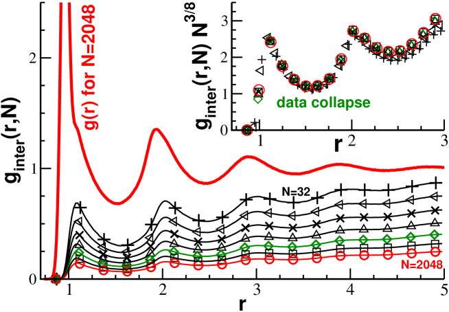
Figure 12: Radial pair correlation function $g_{\text{inter}}(r,N)$ between monomers on different chains using the same symbols as in Fig. 8 for the chain length $N$. Also indicated is the pair correlation function $g(r)$ between all monomers for $N=2048$ (solid line). Measuring the probability that a monomer is close to the chain perimeter $g_{\text{inter}}(r,N)$ decreases strongly with $N$. This decay is perfectly described by $g_{\text{inter}}(r,N)\sim N^{-\nu\Theta_{2}}=1/N^{3/8}$ as shown by the scaling collapse of the data presented in the inset.

A method allowing to verify the fractal dimension of the chain contour not requiring such an artificial parameter is presented in Fig. 12. We show here the radial pair correlation function $g_{\text{inter}}(r,N)$ between monomers on different chains as a function of the distance $r$ between the monomers. The bold line indicates the pair correlation function $g(r)$ between all monomers already presented in Fig. 3. The same normalization is used for $g_{\text{inter}}(r,N)$ as for $g(r)$, i.e. $g_{\text{inter}}(r,N)\to 1$ for large distances where both monomers must necessarily stem from different chains. Obviously, $g(r)\geq g_{\text{inter}}(r,N)$ for all distances $r$. For small distances $r\approx 1$ the pair correlation function $g_{\text{inter}}(r,N)$ measures the probability that two monomers from different chains are in contact. We remind that for open chains, e.g. self-avoiding chains in 3D melts, $g_{\text{inter}}(r,N)$ becomes rapidly chain length independent. Our chains are compact, however, and only a fraction of the chain monomers is close to its contour. Hence, $g_{\text{inter}}(r,N)$ must decrease with $N$ for $r\approx 1$. This is clearly confirmed by the data presented in the main panel. From Eq. (21) we know already the probability for two monomers from different chains to be close to each other, i.e. for both monomers to be close to the chain contour. One expects thus to find

$$g_{\text{inter}}(r,N)\sim L(N)/N\sim N^{-\nu\Theta_{2}}\sim N^{-3/8}$$ (22)

for small distances $r$ of the order of a few monomer diameters. This scaling is perfectly demonstrated by the data collapse presented for all chain lengths in the inset of Fig. 12.

III.7 Intrachain structure factor

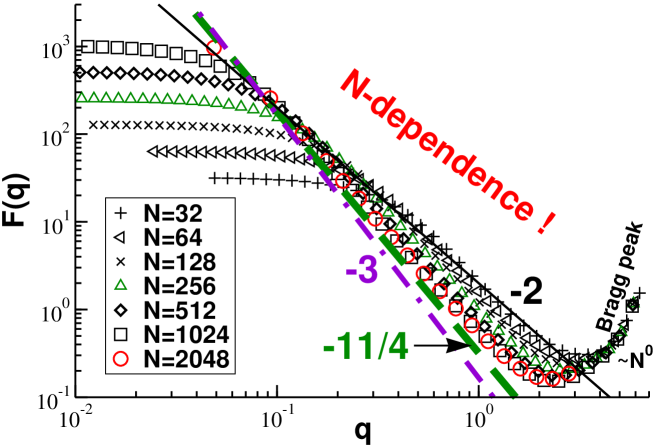
Figure 13: Intramolecular structure factor $F(q)$ as a function of wave vector $q$ for different chain lengths $N$ as indicated. In striking contrast to 3D melts $F(q)$ becomes chain length independent only for wave vectors corresponding to the monomer scale (“Bragg peak”). To characterize the decay in the intermediate wave vector regime our data is compared with three power-law exponents $-2$, $-11/4$ and $-3$ indicated by the thin, the bold dashed line and the dash-dotted line, respectively. The first exponent corresponds to Eq. (23), the second exponent to Eq. (4) and the last exponent to Eq. (24), i.e. to the Porod scattering of a compact 2D object with smooth surface ($d=2,d_{\mathrm{p}}=1$).

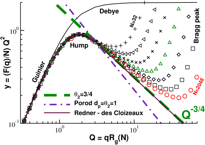
Figure 14: Kratky representation of the structure factor $F(q)$ tracing $y=(F(q)/N)Q^{2}$ as a function of the reduced wave vector $Q=qR_{\text{g}}(N)$ for different $N$ using the same symbols as in Fig. 13. The Debye formula (top thin line) corresponds to a plateau for $Q\gg 1$. At variance to this a strong non-monotonous behavior is revealed by our data which approaches with increasing $N$ a power law exponent $-\Theta_{2}=-3/4$ (dashed line) corresponding to a compact object of fractal line dimension $d_{\mathrm{p}}=d-\theta_{2}=5/4$. The Porod scattering for a compact 2D object with smooth perimeter is given by the dash-dotted line, the Fourier transform of the Redner-des Cloizeaux approximation by the solid line.

Neither the intrachain size distributions $G_{i}(r,s)$, nor the bond-bond correlation functions $P_{1}(s)$ and $P_{2}(s)$ or the contour length $L(s)$ are readily accessible experimentally, at least not for classical small-monomer polymers which cannot be visualized directly by means of fluorescence microscopy or atomic force microscopy. It is thus important to demonstrate that $\Theta_{2}$ is measurable in principle from an analysis of the intrachain structure factor $F(q)=\frac{1}{N}\sum_{n,m=1}^{N}\langle\exp\left[i\mathbf{q}\cdot(\mathbf{r}_{n}-\mathbf{r}_{m})\right]\rangle$ as announced in Eq. (4) in the Introduction and as shown now in Fig. 13 and Fig. 14.

Figure 13 presents the unscaled structure factors $F(q)$ as a function of the wave vector $q$ for a broad range of chain lengths $N$ as indicated. As one expects, $F(q)$ becomes constant for very small wave vectors ($F(q)\to N$), decreases in an intermediate wave vector regime ($R_{\text{g}}(N)\ll 1/q\ll 1$) and shows finally the non-universal monomer structure for large $q$ comparable to the inverse monomeric size (“Bragg peak”). The first striking result of this plot is that $F(q)$ does not become chain length independent in the intermediate wave vector regime as it does for (uncollapsed) polymer chains in 3D. The second observation to be made is that with increasing chain length the decay becomes stronger than the power-law exponent $-2$ indicated by the thin line corresponding to Gaussian chain statistics.

Since for an open polymer-like aggregate or cluster of inverse fractal dimension $\nu$ without any sharp surface the structure factor must indeed scale as de Gennes (1979); Higgins and Benoît (1996)

$$F(q)\sim N^{0}q^{-1/\nu}\mbox{ for }q\gg 1/R_{\text{g}}(N)$$ (23)

several authors Carmesin and Kremer (1990); Maier and Rädler (1999); Polanowski and Pakula (2002); Yethiraj (2003) have argued that an exponent $-2$ should be observed for 2D polymer melts. However, Eq. (23) does not hold for compact structures where strong composition fluctuations (of the labeled monomers of the reference chain with respect to unlabeled monomers) at a thus well-defined surface or perimeter must dominate the structure factor leading to a “generalized Porod scattering” Higgins and Benoît (1996). Since the exponent $\nu=1/2$ for 2D melts does not refer to their Gaussian open chain statistics but rather to their compactness, Eq. (23) is thus inappropriate. Quite generally, the scattering intensity $NF(q)$ of compact objects is known to be proportional to their “surface” $L(N)$ which implies Higgins and Benoît (1996); Bale and Schmidt (1984); Wong and Bray (1988)

$$NF(q)\approx N^{2}/\left(qR(N)\right)^{2d-d_{\mathrm{p}}}\sim R(N)^{d_{\mathrm{p}}}\sim L(N)$$ (24)

where we have used that $R(N)\sim N^{1/d}$ and $R(N)^{d_{\mathrm{p}}}\sim L(N)$. For a 2D object with a smooth perimeter, i.e. for $d_{\mathrm{p}}=1$, this corresponds to the well-known Porod scattering $F(q)\sim q^{-3}$. As indicated by the dash-dotted line in Fig. 13, this yields a too strong decay not compatible either with our data. Obviously, this is to be expected since we already know from Sec. III.6 that the perimeter is fractal ($d_{\mathrm{p}}>1$) and the power-law slope $-3$ must be a lower bound to our data. If we assume, on the contrary, in Eq. (24) a fractal line dimension $d_{\mathrm{p}}=d-\Theta_{2}$, as demonstrated analytically in Eq. (21), this yields directly the key result Eq. (4) anticipated in the Introduction. Using $\Theta=3/4$ we thus have $F(q)\sim q^{-11/4}$ as indicated by the dashed line. This power law gives a reasonable fit for the largest chains we have computed.

The representation of the structure factor used in Fig. 13 is not the best one to check the asymptotic power-law exponents and does not allow to verify the $N$-scaling implied by Eq. (24). We have thus replotted our data in Fig. 14 using a Kratky representation with vertical axis $y=(F(q)/N)Q^{2}$ and a reduced wave vector $Q=qR_{\text{g}}(N)$. Using the measured radius of gyration $R_{\text{g}}(N)$ given in the Table this obviously allows to collapse all data in the Guinier regime for $Q\ll 1$ where Doi and Edwards (1986)

$$y(Q)=Q^{2}\left(1-\frac{Q^{2}}{d}\right).$$ (25)

The observed data collapse is, however, much broader in $Q$ and the more the larger the chain length. The deviations observed for large $Q$ are due to (chain length independent) physics on scales corresponding to the monomer size (“Bragg peak”) already seen in Fig. 13. The Debye formula for Gaussian chains Doi and Edwards (1986) is given by the thin line which becomes constant in this representation for $Q\gg 1$ in agreement with Eq. (23). At variance to this, a striking decay of $y(Q)$ is observed over a decade in $Q$ confirming observations by Yethiraj Yethiraj (2003) and Cavallo et al. Cavallo et al. (2005b) using much shorter chains. Due to the scaling of $y(Q)$ as a function of $Q$ this decay implies the chain length dependence seen for the unscaled structure factor in Fig. 13. With increasing chain length our data approaches systematically the power law $y(Q)\sim Q^{-\Theta_{2}}$ given by Eq. (4) and indicated by the dashed line. Even longer chains obviously are warranted to unambiguously show the predicted asymptotic exponent $-3/4$ in a computer experiment.

In the preceding two paragraphs we have used the fractal line dimension $d_{\mathrm{p}}=d-\Theta_{2}$ derived via Eq. (21) together with the generalized Porod scattering scaling Eq. (24) to demonstrate the key result Eq. (4). Interestingly, the structure factor can be computed directly without the scaling argument Eq. (21) using that $G_{\text{e}}(r,s)\approx G_{2}(r,s)$ for $s\ll N$ as discussed at the end of Sec. III.2. For asymptotically long chains the structure factor thus can be well approximated as

$$F(q)\approx\frac{1}{N}\int_{0}^{N}ds\ 2(N-s)G_{2}(q,s)$$ (26)

using the Fourier transform $G_{2}(q,s)$ of $G_{2}(r,s)$. Within the Redner-des Cloizeaux approximation, Eq. (8), this yields an analytic formula, Eq. (41), given in the Appendix. Readily computed numerically, this theoretical prediction is represented by the solid line in Fig. 14. Since Eq. (8) and Eq. (26) are both approximations this result is not strictly rigorous. However, by construction our formula must yield the Guinier regime, Eq. (25), for small $Q=qR_{\text{g}}(N)$ and since for large $Q$ only the $\Theta_{2}$-exponent matters for large $N$ it is only around the hump $Q\approx 2$ where deviations could be relevant. Fig. 14 shows that in practice our approximation agrees well for all $Q$ as long as the wave vector $q$ does not probe local physics (Bragg regime).

As shown in the Appendix, the Redner-des Cloizeaux approximation Eq. (41) reduces to a power law for wave vectors $Q\gg 1$ corresponding to the power-law regime of Eq. (7),

$$y(Q)\approx\frac{2}{\Gamma(2-\Theta_{2}/2)}\left(\frac{3}{2+\Theta_{2}}\right)^{-(1+\Theta_{2}/2)}Q^{-\Theta_{2}}\approx\frac{1.98}{Q^{3/4}},$$ (27)

in agreement with the key Eq. (4) given in the Introduction. Equation (27) is represented by the dashed lines in Fig. (13) and Fig. (14). Comparing Eq. (24) with Eq. (27) demonstrates that 2D melts are characterized by a fractal line dimension

$$d_{\mathrm{p}}=d-\Theta_{2}=5/4.$$ (28)

Hence, using a slightly more physical route as the scaling argument given in Sec. III.6 we have confirmed the fractal line dimension of the chain perimeter $L(N)$. By labeling only the monomers of sub-chains (which corresponds to a scattering amplitude $sF(q)\sim L(s)\sim R(s)^{d_{\mathrm{p}}}$) the above argument is readily generalized to the perimeter length $L(s)$ of arbitrary segments of length $s\leq N$.

IV Conclusion

Using scaling arguments and molecular dynamics simulation of a well-known model Hamiltonian we investigated various static properties of linear polymer melts in two dimensions. We have shown that the chains adopt compact conformations ($\nu=1/d=1/2$). Due to the segregation of the chains the ratio of end-to-end distance $R_{\text{e}}(N)$ and gyration radius $R_{\text{g}}(N)$ becomes $R_{\text{e}}^{2}(N)/R_{\text{g}}^{2}(N)\approx 5.3<6$ (Fig. 6) and the chains are more spherical than Gaussian phantom chains (Fig. 9). More importantly, it is shown that the irregular chain contours can be characterized by a fractal line dimension $d_{\mathrm{p}}=d-\Theta_{2}=5/4$ (Figs. 10 and 12). This key result has been demonstrated analytically using two different scaling arguments given in Sec. III.6 and Sec. III.7, both based on the numerically tested power-law scaling of the intrachain size distribution $G_{\text{e}}(r,s)\approx G_{2}(r,s)\sim r^{\Theta_{2}}$ for small distances $r\ll R_{\text{e}}(s)$ with $\Theta_{2}=3/4$ (Fig. 5). Compactness and perimeter fractality repeat for subchains of arc-lengths $s$ down to a few monomers due to the self-similar structure of the chains (Figs. 2,4 and 10). Measuring directly the return probability of the chain after $s$ steps, the second Legendre polynomial $P_{2}(s)$ of the bond vectors decays as $P_{2}(s)\sim 1/s^{1+\nu\Theta_{2}}$ (Fig. 8). Interestingly, as implied by the generalized Porod scattering of a compact object with fractal “surface”, Eq. (24), the predicted fractal line dimension should in principle be accessible experimentally from the power-law scaling, Eq. (4), of the intrachain structure factor $F(q)$ in the intermediate wave vector regime. Computationally very demanding systems with chain lengths up to $N=2048$ have been required to test the proposed scaling of the structure factor (Fig. 14).

We would like to stress that our results are not restricted to a particular melt density, but should also hold for all densities provided that the chains are sufficiently long to allow a renormalization of all length scales in terms of semidilute blobs de Gennes (1979). This is of some interest since chain conformations of semidilute 2D solutions of large-monomer polymers (such as DNA or brushlike polymers) are experimentally better accessible than dense melts Maier and Rädler (1999); Sun et al. (2007). Obviously, these macromolecules are rather rigid and in view of the typical molar masses currently used, deviations are to be expected from the asymptotic chain length behavior we focused on. Following previous computational work Carmesin and Kremer (1990); Nelson et al. (1997); Polanowski and Pakula (2002); Yethiraj (2003); Yethiraj et al. (2005); Gavranovic et al. (2005) it should thus be rewarding to reinvestigate the scaling of flexible and semiflexible chains in 2D semidilute solutions to see how finite-$N$ effects may systematically be taken into account.

Interestingly, the fractality of the perimeter precludes a finite line tension and the shape fluctuations of the segments are not suppressed exponentially Carmesin and Kremer (1990), but may occur by advancing and retracting “lobes” in an “amoeba-like” fashion. This opens the possibility for a relaxation mechanism, specific to 2D polymer melts, in which energy is dissipated by friction at the boundary between subchains. Following a suggestion made recently Semenov and Johner (2003), the longest relaxation time $\tau(s)$ of a chain segment should, hence, scale as

$$\tau(s)\sim L(s)^{3}\sim s^{\alpha}\mbox{ with }\alpha=3(1-\nu\Theta_{2})=15/8$$ (29)

rather than with $\alpha=2$ as predicted by the Rouse model which is based on Gaussian chain statistics Doi and Edwards (1986). As Gaussian chain statistics is inappropriate to describe conformational properties of 2D melts, there is no reason why a modeling approach based on this statistics may allow to describe, e.g., the composition fluctuations at the chain contour. Since the latter can in principle be probed experimentally using the dynamical intrachain structure factor $F(q,t)$ Higgins and Benoît (1996) this is an important issue we are currently investigating.

Appendix A Calculation of intrachain structure factor

The intramolecular structure factor $F(q)$ may be rewritten generally as Wittmer et al. (2007)

$$F(q)=\frac{1}{N}\int_{0}^{N}ds\ 2(N-s)G_{\text{e}}(q,s)$$ (30)

using the Fourier transform $G_{\text{e}}(q,s)$ of the two-point intramolecular correlation function $G_{\text{e}}(r,s)$ averaging over all pairs of monomers $(n,m=n+s-1)$ discussed in Sec. III.2. As we have seen in Sec. III.2, $G_{\text{e}}(r,s)$ is well approximated by the distribution $G_{2}(r,s)$ for $s\ll N$. For asymptotically long chains it is justified to neglect chain-end effects ($s\to N$), i.e. physics described by the contact exponents $\Theta_{0}$ and $\Theta_{1}$. Assuming thus translational invariance along the chain contour the structure factor is given approximately by

$$F(q)\approx\frac{1}{N}\int_{0}^{N}ds\ 2(N-s)G_{2}(q,s),$$ (31)

the factor $2(N-s)$ counting the number of equivalent monomer pairs separated by an arc-length $s$. Using the Redner-des Cloizeaux approximation, Eq. (8), for $i=2$ we compute first the 2D Fourier transform

$$G_{2}(q,s)=\int_{0}^{\infty}c_{2}x^{\Theta_{2}}e^{-k_{2}x^{2}}\ 2\pi xdxJ_{0}(qx)$$ (32)

with $2\pi J_{0}(z)=2\int_{0}^{\infty}\cos(z\cos(\theta))d\theta$ being an integer Bessel function Abramowitz and Stegun (1964) and $x=r/R_{2}(s)=r/b_{\text{e}}s^{1/2}$, $\Theta_{2}=3/4$, $k_{2}=1+\Theta_{2}/2$, $c_{2}=k_{2}^{k_{2}}/\pi\Gamma(k_{2})$ as already defined in Sec. III.2. As can be seen from Eq. (11.4.28) of Ref. Abramowitz and Stegun (1964), this integral is given by a standard confluent hypergeometric function, the Kummer function $M(a,b,-z)$,

$$G_{2}(q,s)=M(1+\Theta_{2}/2,1,-z)$$ (33)

with $z=q^{2}b_{\text{e}}^{2}s/4k_{2}$. According to Eq. (13.1.2) and Eq. (13.1.5) of Abramowitz and Stegun (1964) the Kummer function can be expanded as

$$M(a,b,-z) \approx 1-\frac{az}{b}\mbox{ for }|z|\ll 1,$$ (34)

$$M(a,b,-z) \approx \frac{\Gamma(b)}{\Gamma(b-a)}z^{-a}\mbox{ for }z\gg 1.$$ (35)

Using Eq. (33) this yields, respectively, the small and the large wave vector asymptotic behavior of the Fourier transform of $G_{2}(r,s)$

$$G_{2}(q,s) \approx 1-(1+\Theta_{2}/2)z\mbox{ for }z\ll 1,$$ (36)

$$G_{2}(q,s) \approx \frac{\Gamma(1)}{\Gamma(-\Theta_{2}/2)}z^{-(1+\Theta_{2}/2)}\sim q^{-(2+\Theta_{2})}\mbox{ for }z\gg 1.$$ (37)

Note that Eq. (36) implies $G_{2}(q=0,s)=1$ as one expects due to the normalization of $G_{2}(r,s)$.

After integrating over $s$ following Eq. (31) and defining $Z=q^{2}b_{\text{e}}^{2}N/4k_{2}$ one obtains for the Guinier regime of the structure factor

$$F(q)\approx N\left(1-\frac{1+\Theta_{2}/2}{3}Z\right)\mbox{ for }Z\ll 1,$$ (38)

i.e. according to Eq. (25) we have, as one expects,

$$R_{\text{g}}^{2}(N)=\frac{1}{6}b_{\text{e}}^{2}N\frac{1+\Theta_{2}/2}{k_{2}}=\frac{b_{\text{e}}^{2}N}{6}.$$ (39)

This is consistent with Eq. (12) and the ratio $(b_{\text{e}}/b_{\text{g}})^{2}=6$ with $b_{\text{e}}$ determined from subchains with $s\ll N$, Eq. (11). Eq. (39) is of course slightly at variance with the measured ratio $(R_{\text{e}}(N)/R_{\text{g}}(N))^{2}=(b_{\text{e}\star}/b_{\text{g}})^{2}<6$ due the end-effects not taken into account in Eq. (31). The power law behavior of the structure factor for large wave vectors announced in Eq. (4) is obtained by integrating Eq. (37) with respect to $s$. This gives

$$F(q)\approx\frac{2N}{\Gamma(2-\Theta_{2}/2)}Z^{-(1+\Theta_{2}/2)}\sim N^{-\Theta_{2}/2}q^{-(2+\Theta_{2})}\mbox{ for }Z\gg 1.$$ (40)

Obviously, it is also possible to directly integrate Eq. (33) with respect to $s$ according to Eq. (31). This yields the complete Redner-des Cloizeaux approximation of the structure factor

$$\frac{F(q)}{N} \approx 2M\left(1+\frac{\Theta_{2}}{2},2,-Z\right)$$ (41)

$$- M\left(1+\frac{\Theta_{2}}{2},3,-Z\right)$$

$$+ \frac{1}{3}\left(1+\frac{\Theta_{2}}{2}\right)Z\ M\left(2+\frac{\Theta_{2}}{2},4,-Z\right)$$

which can be computed numerically. Using again the expansions of the Kummer function, Eq. (34) and Eq. (35), one verifies readily that Eq. (41) yields the asymptotics for small and large wave vectors already given above. It is convenient from the scaling point of view to replace the variable $Z$ used above by the reduced wave vector $Q=qR_{\text{g}}(N)$ substituting

$$Z\Longrightarrow\frac{6}{4}Q^{2}(1+\Theta_{2}/2)=\frac{12}{11}Q^{2},$$ (42)

as suggested by Eq. (39). This gives the curve represented by the solid line in Fig. 14. Eq. (40) reexpressed in these terms is given by Eq. (27) in the main text. Note that due to this substitution the Guinier limit of the Redner-des Cloizeaux approximation of the structure factor is correct by construction.

$N$	$R_{\text{e}}$	$R_{\text{g}}$	$\left(\frac{R_{\text{e}}}{R_{\text{g}}}\right)^{2}$	$\frac{\left<\lambda_{1}\right>}{\left<\lambda_{2}\right>}$	$\Delta_{1}$	$\Delta_{2}$	$\frac{L(N)}{N}$	$\frac{\delta L(N)}{L(N)}$
32	8.1	3.4	5.7	4.9	0.66	0.56	0.55	0.21
64	11.7	5.0	5.4	4.7	0.65	0.54	0.44	0.22
128	16.7	7.2	5.4	4.6	0.64	0.54	0.35	0.23
256	23.8	10.3	5.3	4.5	0.64	0.53	0.27	0.23
512	34.0	14.7	5.3	4.5	0.64	0.53	0.21	0.23
1024	48.2	20.8	5.3	4.5	0.63	0.52	0.16	0.23
2048	66.4	28.9	5.3	4.4	0.62	0.51	0.13	0.23

Table 1: Various conformational properties defined in the main text for 2D polymers at monomer number density $\rho=7/8$ as a function of chain length $N$. The aspherity of the chains is characterized by the aspect ratio $\left<\lambda_{1}\right>/\left<\lambda_{2}\right>$ and the moments $\Delta_{1}$ and $\Delta_{2}$ of the eigenvalues $\lambda_{1}$ and $\lambda_{2}$ of the inertia tensor. Note that $R_{\text{g}}^{2}=\left<\lambda_{1}\right>+\left<\lambda_{2}\right>$. The mean perimeter length $L(N)$ and its relative fluctuation $\delta L(N)/L(N)$ given in the two last columns have been obtained assuming a reference distance $a=1.2$ (as indicated in Fig. 3) within which at least one monomer from another chain is to be found to identify a monomer as a perimeter monomer.

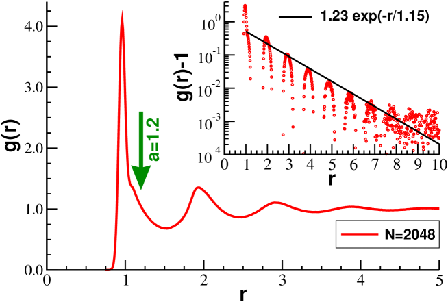
Figure 3: Radial pair correlation function $g(r)$ between all monomers for chains of length $N=2048$ at monomer number density $\rho=7/8$. Note that $g(r)\to 1$ for large monomer distances $r$. The correlation function oscillates strongly with a period given by the bead diameter $\sigma=1$. As shown in the inset, the amplitude of these oscillations decays exponentially as expected for a dense liquid without long-range positional order Chaikin and Lubensky (1995). The arrow indicates the position of the reference length $a=1.2$ used for identifying a monomer as being in contact with a monomer from another chain or subchain.

References

- de Gennes (1979) P. G. de Gennes, Scaling Concepts in Polymer Physics (Cornell University Press, Ithaca, New York, 1979).
- Duplantier (1989) B. Duplantier, J. Stat. Phys. 54, 581 (1989).
- Semenov and Johner (2003) A. N. Semenov and A. Johner, Eur. Phys. J. E 12, 469 (2003).
- Jakobson et al. (2003) J. Jakobson, N. Read, and H. Saleur, Phys. Rev. Lett. 90, 090601 (2003).
- Baumgärtner (1982) A. Baumgärtner, Polymer 23, 334 (1982).
- Carmesin and Kremer (1990) I. Carmesin and K. Kremer, J. Phys. France 51, 915 (1990).
- Ostrovsky et al. (1997) B. Ostrovsky, M. Smith, and Y. Bar-Yam, Int. J. Modern Physics C 8, 931 (1997).
- Nelson et al. (1997) P. Nelson, T. Hatton, and G. Rutledge, Polymer Science Series A 107, 1269 (1997).
- Polanowski and Pakula (2002) P. Polanowski and T. Pakula, J. Chem. Phys. 117, 4022 (2002).
- Balabaev et al. (2002) N. Balabaev, A. Darinskii, I. Neelov, N. Lukasheva, and I. Emri, Polymer Science Series A 44, 781 (2002).
- Yethiraj (2003) A. Yethiraj, Macromolecules 36, 5854 (2003).
- Yethiraj et al. (2005) A. Yethiraj, B. J. Sung, and F. Lado, J. Chem. Phys. 122, 094910 (2005).
- Cavallo et al. (2003) A. Cavallo, M. Müller, and K. Binder, Europhys. Lett. 61, 214 (2003).
- Cavallo et al. (2005a) A. Cavallo, M. Müller, and K. Binder, J. Phys. Chem. B 109, 6544–6552 (2005a).
- Cavallo et al. (2005b) A. Cavallo, M. Müller, J. P. Wittmer, A. Johner, and K. Binder, J. Phys.: Condens. Matter 17, S1697 (2005b).
- Meyer et al. (2009) H. Meyer, T. Kreer, M. Aichele, A. Cavallo, A. Johner, J. Baschnagel, and J. Wittmer, Phys. Rev. E 79, 050802(R) (2009).
- Maier and Rädler (1999) B. Maier and J. O. Rädler, Phys. Rev. Lett. 82, 1911 (1999).
- Wang and Foltz (2004) X. Wang and V. J. Foltz, J. Chem. Phys. 121, 8158 (2004).
- Gavranovic et al. (2005) G. T. Gavranovic, J. Deutsch, and G. Fuller, Macromolecules 38, 6672 (2005).
- Sun et al. (2007) F. Sun, A. Dobrynin, D. Shirvanyants, H. Lee, K. Matyjaszewski, G. Rubinstein, M. Rubinstein, and S. Sheiko, Phys. Rev. Lett. 99, 137801 (2007).
- Zhao and Granick (2007) J. Zhao and S. Granick, Macromolecules 40, 1243 (2007).
- Srivastava and Basu (2009) S. Srivastava and J. Basu, J. Comp. Phys. 130, 224907 (2009).
- Maier and Rädler (2000) B. Maier and J. O. Rädler, Macromolecules 33, 7185 (2000).
- Maier and Rädler (2001) B. Maier and J. O. Rädler, Macromolecules 34, 5723 (2001).
- Mandelbrot (1982) B. Mandelbrot, The Fractal Geometry of Nature (W.H. Freeman, San Francisco, California, 1982).
- Higgins and Benoît (1996) J. Higgins and H. Benoît, Polymers and Neutron Scattering (Oxford University Press, Oxford, 1996).
- Bale and Schmidt (1984) H. D. Bale and P. W. Schmidt, Phys. Rev. Lett. 53, 596 (1984).
- Wong and Bray (1988) P. Z. Wong and A. J. Bray, Phys. Rev. Lett. 60, 1344 (1988).
- Grest and Kremer (1986) G. S. Grest and K. Kremer, Phys. Rev. A 33, 3628 (1986).
- Kremer and Grest (1990) K. Kremer and G. Grest, J. Chem. Phys. 92, 5057 (1990).
- Dünweg (1993) B. Dünweg, J. Chem. Phys. 99, 61 (1993).
- Attig et al. (2004) N. Attig, K. Binder, H. Grubmüller, and K. Kremer, eds., Computational Soft Matter: From Synthetic Polymers to Proteins, vol. 23 (NIC Series, Jülich, 2004).
- Frenkel and Smit (2002) D. Frenkel and B. Smit, Understanding Molecular Simulation – From Algorithms to Applications (Academic Press, San Diego, 2002), 2nd edition.
- Chaikin and Lubensky (1995) P. M. Chaikin and T. C. Lubensky, Principles of condensed matter physics (Cambridge University Press, 1995).
- Plimpton (1995) S. J. Plimpton, J. Comp. Phys. 117, 1 (1995).
- Doi and Edwards (1986) M. Doi and S. F. Edwards, The Theory of Polymer Dynamics (Clarendon Press, Oxford, 1986).
- Wittmer et al. (2007) J. P. Wittmer, P. Beckrich, H. Meyer, A. Cavallo, A. Johner, and J. Baschnagel, Phys. Rev. E 76, 011803 (2007).
- Wittmer et al. (2004) J. P. Wittmer, H. Meyer, J. Baschnagel, A. Johner, S. P. Obukhov, L. Mattioni, M. Müller, and A. N. Semenov, Phys. Rev. Lett. 93, 147801 (2004).
- Auhl et al. (2003) R. Auhl, R. Everaers, G. Grest, K. Kremer, and S. Plimpton, J. Chem. Phys. 119, 12718 (2003).
- des Cloizeaux and Jannink (1990) J. des Cloizeaux and G. Jannink, Polymers in Solution : their Modelling and Structure (Clarendon Press, Oxford, 1990).
- Abramowitz and Stegun (1964) M. Abramowitz and I. A. Stegun, Handbook of Mathematical Functions (Dover, New York, 1964).
- Everaers et al. (1995) R. Everaers, I. Graham, and M. Zuckermann, J. Phys. A 28, 1271 (1995).
- Bishop and Satiel (1986) M. Bishop and C. J. Satiel, J. Chem. Phys. 85, 6728 (1986).
- Rudnick and Gaspari (1986) J. Rudnick and G. Gaspari, J. Phys. A 19, L191 (1986).
- Aronovitz and Nelson (1986) J. Aronovitz and D. Nelson, J. Phys. (Paris) 47, 1445 (1986).