A self-consistent quantum master equation approach to molecular transport

Abstract

We propose a self-consistent generalized quantum master equation (GQME) to describe electron transport through molecular junctions. In a previous study [M.Esposito and M.Galperin. Phys. Rev. B 79, 205303 (2009)], we derived a time-nonlocal GQME to cure the lack of broadening effects in Redfield theory. To do so, the free evolution used in the Born-Markov approximation to close the Redfield equation was replaced by a standard Redfield evolution. In the present paper, we propose a backward Redfield evolution leading to a time-local GQME which allows for a self-consistent procedure of the GQME generator. This approach is approximate but properly reproduces the nonequilibrium steady state density matrix and the currents of an exactly solvable model. The approach is less accurate for higher moments such as the noise.

I Introduction

Recent advances in the experimental capabilities for constructing molecular junctions and measuring their response to external perturbations create new challenges for an adequate theoretical description of open quantum systems far from equilibrium.Nitzan and Ratner (2003); Lindsay and Ratner (2007); Galperin et al. (2007); Galperin et al. (2008a) In molecular junctions, most of the interesting applications are concerned with either strongly correlated or resonant tunneling regimes (or both). In these situations, conventional perturbation theory and/or effective mean-field theories (e.g. Hartree-Fock, GW, DFT) are inapplicable and may lead to unphysical predictions.Spataru et al. (2009)

In molecular junctions, molecules are sensible to processes such as oxidation, reduction, and excitations. This makes the description of transport in the language of the many-body states of the isolated molecules a convenient tool for molecules weakly coupled to the contacts. Furthermore, sophisticated quantum chemistry methods use many-body states to describe molecular electronic structures.Jensen (2007) The dressed state representation,Nitzan (2006) often employed in quantum chemistry, is another example of many-body states formulation. The standard nonequilibrium Green function (NEGF) approach,Danielewicz (1984); Rammer and Smith (1986); Haug and Jauho (2008) is formulated in the language of elementary excitations and is therefore not well suited for a many-body states description. A suitable alternative, the Hubbard NEGF approach, Sandalov et al. (2003); Fransson (2005); Galperin et al. (2008b) still displays inconsistencies for low level of approximation that need to be resolved (see Ref. Galperin et al., 2008b for a discussion).

The simplest approach to transport at the molecular state level is the Redfield quantum master equation (QME) originally developed in the context of NMRRedfield (1957) and later in many other fieldsNitzan (2006); Breuer and Petruccione (2002); Gaspard and Nagaoka (1999) including transport through quantum junctions.Li et al. (2005); Harbola et al. (2006); Schultz and von Oppen (2009) It is derived using the Born-Markov approximation in order to get a closed evolution equation for the reduced density matrix. The rotating wave (or secular) approximation (RWA)Breuer and Petruccione (2002); Harbola et al. (2006) is often invoked when the molecular levels are well separated so that the molecule Bohr frequencies evolve fast compared to the relaxation time scale induced by the coupling to the contact. This leads to a QME which has a simple physical interpretation in the molecular eigenbasis. Indeed, populations satisfy a rate equation with rates given by Fermi golden rule (Pauli equation) and the coherences are each independently exponentially damped. As a result, in nonequilibrium steady-states, all coherence effects (in the molecular eigenbasis) are lost. In its general form, the Markovian Redfield equation predicts steady-state coherences that can be inaccurate and even sometimes lead to unphysical results.Kohen and Tannor (1997); Kohen et al. (1997); Harbola et al. (2006); Ishizaki and Fleming (2009) Furthermore, broadening effects are totally absent from the Redfield description.Pedersen and Wacker (2005); Ovchinnikov and Neuhauser (2004); Leijnse and Wegewijs (2008); Esposito and Galperin (2009). In order to overcome some of these difficulties, we proposed in our previous workEsposito and Galperin (2009) a generalized QME capable of predicting the broadening of the molecular levels in an approximate way. The key idea was to replace the assumption of free molecular evolution inside the kernel (which is second order in the molecule-contact interaction) used in the Born-Markov approximation by the Redfield evolution. The resulting equation was however non-local in time. Here we extend our consideration by proposing a kind of time-reversed Redfield evolution that leads to a time local generalized QME. This procedure is rewarding because it allows to formulate a practical self-consistent scheme to calculate the generator of the QME.

The structure of the paper is the following. Section II introduces a model of molecular junction. In section III, we briefly review our generalized QME derived earlier and introduce the self-consistent scheme. Section IV presents numerical examples and compares the results obtained within the scheme to a numerically exact approach. Conclusions are drawn in section V.

II Model

We consider a molecule ($M$) coupled to two metal contacts ($L$ and $R$) each at its own equilibrium. The Hamiltonian of the system is

$$\hat{H}=\hat{H}_{M}+\sum_{K=L,R}\left(\hat{H}_{K}+\hat{V}_{KM}\right)$$ (1)

The contacts are assumed to be reservoirs of free charge carriers

$$\hat{H}_{K}=\sum_{k\in K}\varepsilon_{k}\hat{c}_{k}^{\dagger}\hat{c}_{k}$$ (2)

where $K=L,R$ and $\hat{c}_{k}^{\dagger}$ ($\hat{c}_{k}$) are creation (annihilation) operators for an electron in state $k$.

The molecular Hamiltonian is represented in terms of the many-body states $\{|M\rangle\}$ of the isolated molecule

$$\hat{H}_{M}=\sum_{M_{1},M_{2}}|M_{1}\rangle H^{(M)}_{M_{1}M_{2}}\langle M_{2}|\equiv\sum_{M_{1},M_{2}}H^{(M)}_{M_{1}M_{2}}\hat{X}_{M_{1},M_{2}}$$ (3)

where $\hat{X}_{M_{1},M_{2}}$ are projection (or Hubbard) operators. In particular, in the eigenbasis representation, the molecular Hamiltonian reads

$$\hat{H}_{M}=\sum_{M}E_{M}\hat{X}_{M,M}$$ (4)

where $E_{M}$ are the eigenenergies. Note that the molecular many-body states $|M\rangle$ are characterized by all the relevant quantum numbers describing the state of an isolated molecule or a dressed state.

The coupling between the molecule and the contacts is introduced in the usual way with hopping terms for the electrons moving from the contact to the molecule and vice versa

$$\hat{V}_{KM}=\sum_{k\in K}\sum_{\mathcal{M}}\left(V_{\mathcal{M}k}\hat{X}_{\mathcal{M}}^{\dagger}\hat{c}_{k}+V_{k\mathcal{M}}\hat{c}_{k}^{\dagger}\hat{X}_{\mathcal{M}}\right)$$ (5)

Here

$$\mathcal{M}\equiv(N_{f}\,s_{f},N_{i}\,s_{i})$$ (6)

is a transition from the molecular state $M_{i}\equiv N_{i}\,s_{i}$ to the molecular state $M_{f}\equiv N_{f}\,s_{f}$. The number of electrons on the molecule is $N_{f}=N_{i}-1$ and $s_{i}$ ($s_{f}$) is the set of all the quantum numbers characterizing the molecular state in the charging block $N_{i}$ ($N_{f}$), so that $\hat{X}_{\mathcal{M}}\equiv\hat{X}_{M_{f},M_{i}}$.

III Generalized quantum master equation

In this section we start by reviewing the derivation of the generalized QME introduced in our previous work. We then introduce our new way of closing the master equation by using a time-reversed effective evolution, and demonstrate how the resulting equation can lead to a self-consistent scheme to calculate the propagator of the molecular density matrix.

Exact equation of motion

We start by deriving exact equation of motion (EOM) for the quantity

$$\langle\hat{X}_{21}(t)\rangle\equiv\mbox{Tr}\left[e^{+i\hat{H}(t-t_{0})}\hat{X}_{21}e^{-i\hat{H}(t-t_{0})}\hat{\rho}_{0}\right]\equiv\sigma_{12}(t)$$ (7)

where $|1\rangle$ and $|2\rangle$ are many-body molecular states, $t_{0}$ is a starting point of the evolution usually taken at the infinite past $t_{0}\to-\infty$, and $\hat{\rho}_{0}$ is the initial density operator for the whole system (molecule and contacts). We note that

$$\sigma_{12}(t)\equiv\langle 1|\,\mbox{Tr}_{K}\left[\hat{\rho}(t)\right]\,|2\rangle$$ (8)

is a matrix element of the reduced density operator of the molecule $\hat{\sigma}$ at time $t$ which is obtained by tracing out the contact degrees of freedom from the full density matrix.

The Heisenberg EOM for the Hubbard operator in Eq.(7) yields an exact EOM for the reduced density matrix (see Ref. Esposito and Galperin, 2009 for details of derivation) which in molecular eigenbasis reads

$$\frac{d}{dt}\sigma_{12}(t)=-i\left(E_{1}-E_{2}\right)\sigma_{12}(t)-\sum_{\mathcal{M}}\sum_{s}\int_{-\infty}^{t}dt^{\prime}$$

$$i\left\{(-1)^{N_{1}-N_{2}}\left[\Sigma^{<}_{(N_{1}-1\,s,1)\mathcal{M}}(t-t^{\prime})\langle\hat{X}_{\mathcal{M}}(t^{\prime})\,\hat{X}^{\dagger}_{N_{1}-1\,s,2}(t)\rangle\right.\right.$$

$$\qquad\qquad\left.+\langle\hat{X}_{N_{2}-1\,s,1}(t)\,\hat{X}^{\dagger}_{\mathcal{M}}(t^{\prime})\rangle\Sigma^{<}_{\mathcal{M}(N_{2}-1\,s,2)}(t^{\prime}-t)\right]$$

$$\quad-\Sigma^{<}_{(2,N_{2}+1\,s)\mathcal{M}}(t-t^{\prime})\langle\hat{X}_{\mathcal{M}}(t^{\prime})\,\hat{X}^{\dagger}_{1,N_{2}+1\,s}(t)\rangle$$

$$\quad+\langle\hat{X}^{\dagger}_{\mathcal{M}}(t^{\prime})\,\hat{X}_{N_{2}-1\,s,1}(t)\rangle\Sigma^{>}_{\mathcal{M}(N_{2}-1\,s,2)}(t^{\prime}-t)$$

$$\quad+\Sigma^{>}_{(N_{2}-1\,s,1)\mathcal{M}}(t-t^{\prime})\langle\hat{X}^{\dagger}_{N_{1}-1\,s,2}(t)\,\hat{X}_{\mathcal{M}}(t^{\prime})\rangle$$

$$\quad-\langle\hat{X}_{2,N_{1}+1\,s}(t)\,\hat{X}^{\dagger}_{\mathcal{M}}(t^{\prime})\rangle\Sigma^{<}_{\mathcal{M}(1,N_{1}+1\,s)}(t^{\prime}-t)$$

$$-(-1)^{N_{1}-N_{2}}\left[\Sigma^{>}_{(2,N_{2}+1\,s)\mathcal{M}}(t-t^{\prime})\langle\hat{X}^{\dagger}_{1,N_{2}+1\,s}(t)\,\hat{X}_{\mathcal{M}}(t^{\prime})\rangle\right.$$

$$\left.\left.\qquad\qquad+\langle\hat{X}^{\dagger}_{\mathcal{M}}(t^{\prime})\,\hat{X}_{2,N_{1}+1\,s}(t)\rangle\Sigma^{>}_{\mathcal{M}(1,N_{1}+1\,s)}(t^{\prime}-t)\right]\right\}$$ (9)

Here, $\mathcal{M}$ is defined in Eq.(6), $\Sigma^{>\,(<)}_{\mathcal{M}_{1}\mathcal{M}_{2}}$ are the greater (lesser) projections of a self-energy due to the coupling to the contacts

$$\Sigma_{\mathcal{M}_{1}\mathcal{M}_{2}}(\tau_{1},\tau_{2})\equiv\sum_{K=L,R}\sum_{k\in K}V_{\mathcal{M}_{1}k}\,g_{k}(\tau_{1},\tau_{2})\,V_{k\mathcal{M}_{2}}$$ (10)

where $g_{k}(\tau_{1},\tau_{2})\equiv-i\langle T_{c}\hat{c}_{k}(\tau_{1})\,\hat{c}_{k}^{\dagger}(\tau_{2})\rangle$ is the free electron Green function ($T_{c}$ is the contour ordering operator). Dissipation matrix $\Gamma$ is introduced in a usual way

$$\Gamma_{\mathcal{M}_{1}\mathcal{M}_{2}}(E)=i\left[\Sigma^{r}_{\mathcal{M}_{1}\mathcal{M}_{2}}(E)-\Sigma^{a}_{\mathcal{M}_{1}\mathcal{M}_{2}}(E)\right]$$ (11)

and within wide band approximation assumed below is energy independent.

Eq.(III) is exact but does not have a closed form in terms of the reduced density matrix $\sigma_{12}$. Indeed, its right hand side contains two-time correlation functions of Hubbard operators. Attempt to write EOM for the latter would lead to expressions having in their right hand side correlation functions of higher order involving both, molecular Hubbard operators and creation (annihilation) operators for the electrons in the contacts, at different times. This would generate an infinite hierarchy of EOMs.

Generalized time-nonlocal QME

The usual strategy involves closing the system of equations by approximately representing high order correlation function in terms of correlation function(s) of lower order. In particular, closing Eq.(III) for the case when $M$ are effective single particle orbitals at the first step (i.e. reducing the two-time correlation function in the right hand side to a single time average) is known as the generalized Kadanoff-Baym ansatz (GKBA).Haug and Jauho (2008) In our previous work Esposito and Galperin (2009), we introduced the analogue of the GKBA in Liouville space where $M$ are molecular many-body states:

$$\langle\hat{X}_{12}(t)\hat{X}^{\dagger}_{34}(t^{\prime})\rangle\approx$$

$$i\sum_{M_{1},M_{2}}\left[\mathcal{G}^{r}_{12,M_{1}M_{2}}(t-t^{\prime})\langle\hat{X}_{M_{1}M_{2}}(t^{\prime})\,\hat{X}^{\dagger}_{34}(t^{\prime})\rangle\right.$$ (12)

$$\left.\qquad\quad-\langle\hat{X}_{12}(t)\,\hat{X}^{\dagger}_{M_{1}M_{2}}(t)\rangle\mathcal{G}^{a}_{M_{1}M_{2},34}(t-t^{\prime})\right]$$

A similar expression holds for $\langle\hat{X}^{\dagger}_{34}(t^{\prime})\,\hat{X}_{12}(t)\rangle$. Here $\mathcal{G}^{r\,(a)}$ are retarded (advanced) Green functions in Liouville space

$$\mathcal{G}^{r}_{12,34}(t) \equiv-i\theta(t)\ll\hat{X}_{21}\hat{I}_{B}\rvert e^{-i\mathcal{L}t}\rvert\hat{X}_{43}\hat{\rho}_{B}^{eq}\gg$$

$$\equiv-i\theta(t)\ll\hat{X}_{21}\rvert e^{-i\mathcal{L}_{eff}t}\rvert\hat{X}_{43}\gg$$ (13)

$$\mathcal{G}^{a}_{12,34}(t) \equiv-i\theta(-t)\ll\hat{X}_{34}\hat{I}_{B}\rvert e^{i\mathcal{L}t}\rvert\hat{X}_{12}\hat{\rho}_{B}^{eq}\gg$$

$$\equiv i\theta(-t)\ll\hat{X}_{34}\rvert e^{i\mathcal{L}_{eff}t}\lvert\hat{X}_{12}\gg$$ (14)

where $\hat{\rho}_{B}^{eq}\equiv\hat{\rho}_{L}^{eq}\hat{\rho}_{R}^{eq}$ is the equilibrium density operator for the contacts and $\hat{I}_{B}$ is unity operator in the contacts subspace. Using (III) in (III), leads to a time-nonlocal generalized QME given by Eq.(35) in Ref. Esposito and Galperin, 2009.

Generalized time-local QME

We now propose an alternative way to close Eq.(III) by reducing the two-time correlation function in the right hand side of (III) to the later rather than earlier time. Indeed, since the whole system evolution is time-reversible (one has to be careful with spin and magnetic field, though), and since the reduction of a two-time correlation function to a single-time average is an approximation, the reduction of the correlation function to a later time does not a priori seem to be worse than to the earlier one.

The two-time correlation function can be exactly expressed in Liouville space as

$$\langle\hat{X}_{12}(t)\,\hat{X}^{\dagger}_{34}(t^{\prime})\rangle=$$

$$\qquad\theta(t-t^{\prime})\ll\hat{X}_{34}\hat{I}_{B}\rvert e^{-i\mathcal{L}(t^{\prime}-t)}\lvert\hat{\rho}(t)\hat{X}_{12}\gg$$ (15)

$$\quad+\theta(t^{\prime}-t)\ll\hat{X}_{12}^{\dagger}\hat{I}_{B}\rvert e^{-i\mathcal{L}(t-t^{\prime})}\lvert\hat{X}_{34}^{\dagger}\hat{\rho}(t^{\prime})\gg$$

Then using the projection superoperator introduced in Ref. Esposito and Galperin, 2009

$$\mathcal{P}=\sum_{M_{1},M_{2}}\lvert\hat{X}_{M_{1},M_{2}}\hat{\rho}_{B}^{eq}\gg\,\ll\hat{X}_{M_{1},M_{2}}\hat{I}_{B}\rvert$$ (16)

one gets the alternative ansatz

$$\langle\hat{X}_{12}(t)\hat{X}^{\dagger}_{34}(t^{\prime})\rangle\approx$$

$$i\sum_{M_{1},M_{2}}\left[\tilde{\mathcal{G}}{}^{r}_{12,M_{1}M_{2}}(t-t^{\prime})\langle\hat{X}_{M_{1}M_{2}}(t^{\prime})\,\hat{X}^{\dagger}_{34}(t^{\prime})\rangle\right.$$ (17)

$$\left.\qquad\quad-\langle\hat{X}_{12}(t)\,\hat{X}^{\dagger}_{M_{1}M_{2}}(t)\rangle\tilde{\mathcal{G}}{}^{a}_{M_{1}M_{2},34}(t-t^{\prime})\right]$$

and a similar expression for $\langle\hat{X}^{\dagger}_{34}(t^{\prime})\,\hat{X}_{12}(t)\rangle$. Here we introduced the retarded and advanced Green functions on the Keldysh anti-contourBányai (2006)

$$\tilde{\mathcal{G}}{}^{r}_{12,34}(t) \equiv-i\theta(-t)\ll\hat{X}_{21}\hat{I}_{B}\rvert e^{-i\mathcal{L}t}\rvert\hat{X}_{43}\hat{\rho}_{B}^{eq}\gg$$

$$\equiv-i\theta(-t)\ll\hat{X}_{21}\rvert e^{-i\ {}^{\theta}\mathcal{L}_{eff}t}\rvert\hat{X}_{43}\gg$$ (18)

$$\tilde{\mathcal{G}}{}^{a}_{12,34}(t) \equiv i\theta(t)\ll\hat{X}_{34}\hat{I}_{B}\rvert e^{i\mathcal{L}t}\rvert\hat{X}_{12}\hat{\rho}_{B}^{eq}\gg$$

$$\equiv i\theta(t)\ll\hat{X}_{34}\rvert e^{i\ {}^{\theta}\mathcal{L}_{eff}t}\lvert\hat{X}_{12}\gg$$ (19)

where ${}^{\theta}\mathcal{L}_{eff}$ is the effective Liouvillian generating the time-reversed evolution. Its connection to the effective Liouvillian $\mathcal{L}_{eff}$ generating forward-time evolution isStenholm and Jacob (2004a, b)

$${}^{\theta}\mathcal{L}=\mathcal{L}^{*}$$ (20)

Note difference in sign with Refs. Stenholm and Jacob, 2004a, b which is due to our definition of evolution operator as $e^{-i\ {}^{\theta}\mathcal{L}_{eff}t}$ instead of $e^{{}^{\theta}\mathcal{L}_{eff}t}$ in Refs. Stenholm and Jacob, 2004a, b.

Applying (III) to (III) leads to a time-local version of the generalized QME

$$\frac{d}{dt}\sigma_{12}(t)=\sum_{3,4}\mathcal{L}_{12,34}\,\sigma_{34}(t)$$ (21)

where in the molecular eigenbasis

$$\mathcal{L}_{12,34}=-i(E_{1}-E_{2})\,\delta_{1,3}\,\delta_{2,4}-\sum_{\mathcal{M}}\int_{-\infty}^{+\infty}dt$$

$$\left\{\ (-1)^{N_{1}-N_{2}}\,\delta_{N_{1}-1,N_{3}}\,\delta_{N_{2}-1,N_{4}}\times\right.$$

$$\left[\tilde{\mathcal{G}}{}^{a}_{(3,1)\mathcal{M}}(t)\,\Sigma^{<}_{\mathcal{M}(4,2)}(-t)-\Sigma^{<}_{(3,1)\mathcal{M}}(t)\,\tilde{\mathcal{G}}{}^{r}_{\mathcal{M}(4,2)}(-t)\right]$$

$$-(-1)^{N_{1}-N_{2}}\,\delta_{N_{1}+1,N_{3}}\,\delta_{N_{2}+1,N_{4}}\times$$

$$\left[\tilde{\mathcal{G}}{}^{a}_{(2,4)\mathcal{M}}(t)\,\Sigma^{>}_{\mathcal{M}(1,3)}(-t)-\Sigma^{>}_{(2,4)\mathcal{M}}(t)\,\tilde{\mathcal{G}}{}^{r}_{\mathcal{M}(1,3)}(-t)\right]$$

$$+\delta_{1,3}\,\delta_{N_{2},N_{4}}\sum_{s}\left[\tilde{\mathcal{G}}{}^{a}_{(N_{2}-1\,s,4)\mathcal{M}}(t)\,\Sigma^{>}_{\mathcal{M}(N_{2}-1\,s,2)}(-t)\right.$$

$$\left.\qquad\qquad+\Sigma^{<}_{(2,N_{2}+1\,s)\mathcal{M}}(t)\,\tilde{\mathcal{G}}{}^{r}_{\mathcal{M}(4,N_{2}+1\,s)}(-t)\right]$$

$$-\delta_{2,4}\,\delta_{N_{1},N_{3}}\sum_{s}\left[\tilde{\mathcal{G}}{}^{a}_{(3,N_{1}+1\,s)\mathcal{M}}(t)\,\Sigma^{<}_{\mathcal{M}(1,N_{1}+1\,s)}(-t)\right.$$

$$\left.\left.\qquad\qquad+\Sigma^{>}_{(N_{1}-1\,s,1)\mathcal{M}}(t)\,\tilde{\mathcal{G}}{}^{r}_{\mathcal{M}(N_{1}-1\,s,3)}(-t)\right]\right\}$$ (22)

Note that this expression for the effective Liouvillian in an arbitrary basis will differ from Eq.(III) only in the free evolution term.

If the QME, Eqs. (21) and (III), is used with the free molecular evolution instead of the effective dynamics in Eqs. (III) and (III), one gets the standard Markovian Redfield QME. The RWA is justified when $\Gamma_{mn}\ll|\varepsilon_{a}-\varepsilon_{b}|$ ($m,n\in\{a,b\}$) in the molecular eigenbasis and consist in neglecting the nondiagonal of $\Gamma_{mn}$ (here the standard effective single orbital formulation is used)Harbola et al. (2006). As a result, coherences become decoupled from population in the molecular eigenbasis. The former die off at steady state and later obey a Pauli rate equation. When the RWA is not justified, coherence effects in the molecular eigenbasis cannot be neglected.

It should be clear from our derivation that time-local form Eq.(21) of the generalized QME should have a similar degree of accuracy as the time-nonlocal version proposed earlier.Esposito and Galperin (2009) However, the present form is more suitable for realistic calculations, but most important it naturally suggests a self-consistent procedure to evaluate the effective Liouvillian. Indeed, the effective Liouvillian, Eq.(III), depends on the Liouville space Green functions, Eqs. (III) and (III), which in turn depend on the Liouvillian through the connection (20).

Expression for current

The general expression for the time-dependent current at the contact-molecule interface $K$ can be calculated within the non-equilibrium Hubbard Green function approach asJauho et al. (1994); Galperin et al. (2008b)

$$I_{K}(t) =2\,\mbox{Im}\int_{-\infty}^{t}dt^{\prime}\,\sum_{\mathcal{M},\mathcal{M}^{\prime}}$$

$$\left[\ \langle\hat{X}_{\mathcal{M}}(t)\,\hat{X}^{\dagger}_{\mathcal{M}^{\prime}}(t^{\prime})\rangle\Sigma^{<\,K}_{\mathcal{M}^{\prime}\mathcal{M}}(t^{\prime}-t)\right.$$ (23)

$$\left.+\langle\hat{X}^{\dagger}_{\mathcal{M}^{\prime}}(t^{\prime})\,\hat{X}_{\mathcal{M}}(t)\rangle\Sigma^{>\,K}_{\mathcal{M}^{\prime}\mathcal{M}}(t^{\prime}-t)\right]$$

Using our ansatz, Eq.(III), leads to the expression

$$I_{K}(t)=-2\,\mbox{Re}\int_{-\infty}^{+\infty}dt^{\prime}\sum_{\mathcal{M},\mathcal{M}^{\prime}}\sum_{s}$$ (24)

$$\left[\sigma_{N\,s,N\,s_{f}}(t)\,\tilde{\mathcal{G}}{}^{a}_{(N\,s,N+1\,s_{i})\mathcal{M}^{\prime}}(t-t^{\prime})\,\Sigma^{<\,K}_{\mathcal{M}^{\prime}\mathcal{M}}(t^{\prime}-t)\right.$$

$$\left.+\sigma_{N+1\,s_{i},N+1\,s}(t)\,\tilde{\mathcal{G}}{}^{a}_{(N\,s_{f},N+1\,s)\mathcal{M}^{\prime}}(t-t^{\prime})\,\Sigma^{>\,K}_{\mathcal{M}^{\prime}\mathcal{M}}(t^{\prime}-t)\right]$$

where $\mathcal{M}\equiv(N\,s_{f},N+1\,s_{i})$.

Full counting statistics

The theory of full counting statistics (FCS) was initially proposed by Levitov and Lesovik,Levitov and Lesovik (1993); Levitov et al. (1996) and became popular in the molecular electronics community when shot noise in molecular junctions became experimentally measurable.Djukic and van Ruitenbeek (2006) The theoretical formalism for FCS within the QME was developed in Ref. Esposito et al., 2009. Within the FCS the evolution operator is dressed by counting field(s) $\lambda$ which track the exchange of electrons between the molecule and the contact(s)

$$\hat{V}^{\lambda}_{KM}=\sum_{k\in K}\sum_{\mathcal{M}}\left(V_{\mathcal{M}k}e^{i\lambda/2}\hat{X}_{\mathcal{M}}^{\dagger}\hat{c}_{k}+V_{k\mathcal{M}}e^{-i\lambda/2}\hat{c}_{k}^{\dagger}\hat{X}_{\mathcal{M}}\right)$$ (25)

Below we assume that counting starts at time $t_{0}$.

The dressed Liouville equation for the total density matrix takes the form

$$|\hat{\rho}_{\lambda}(t)\gg=\exp[-i\mathcal{L}_{\lambda}(t-t_{0})]\,|\hat{\rho}(t_{0})\gg$$ (26)

As usual initial condition is assumed to be a direct product of the molecular and bath density matrices

$$|\hat{\rho}(t_{0})\gg=|\hat{\sigma}(t_{0})\,\hat{\rho}_{B}^{eq}\gg$$ (27)

so that dressed evolution of the system DM becomes

$$|\hat{\sigma}_{\lambda}(t)\gg=\exp[-i\mathcal{L}_{eff,\lambda}(t-t_{0})]\,|\hat{\sigma}(t_{0})\gg$$ (28)

The FCS is given by the generating function

$$G(t,\lambda)\equiv\ll\hat{I}|\hat{\rho}_{\lambda}(t)\gg$$ (29)

The long time limit of the logarithm of the generating function,

$$S(\lambda)\equiv\lim_{t\to\infty}\frac{1}{t}\ln G(t,\lambda),$$ (30)

provides information on the steady-state cumulants of the FCS

$$C_{n}\equiv\frac{d^{n}}{d(i\lambda)^{n}}S(\lambda)$$ (31)

In particular, the steady-state current is given by the first cumulant and the second cumulant yields to the zero-frequency shot noise. Using the spectral decomposition of the effective Liouvillian

$$\mathcal{L}_{eff,\lambda}=\sum_{\gamma}|R_{\gamma}(\lambda)\gg\,\nu_{\gamma}(\lambda)\,\ll L_{\gamma}(\lambda)|$$ (32)

and since in the long time limit only one eigenmode $\nu_{0}(\lambda)$ survives, we get

$$I =-\frac{d}{d\lambda}\nu_{0}(\lambda)$$ (33)

$$S =i\frac{d^{2}}{d\lambda^{2}}\nu_{0}(\lambda)$$ (34)

We note that both (24) and (33) provide the same steady-state current.

IV Numerical examples

We now compare the results predicted by our new self-consistent approach with the standard Markovian Redfield equation and the nonequilibrium Green function results. The simplest model which can be treated by these three methods, while providing information on both populations and coherences, is a non-interacting two-level bridge (TLB) between metallic contacts.

The bridge part of the model has 4 many-body states: $\lvert 0\rangle\equiv\lvert 0,0\rangle$, $\lvert a\rangle\equiv\lvert 1,0\rangle$, $\lvert b\rangle\equiv\lvert 0,1\rangle$, and $\lvert 2\rangle\equiv\lvert 1,1\rangle$, where $\lvert n_{a},n_{b}\rangle$ indicates number of electrons $n_{a,b}=\{0,1\}$ on the level $a$ and $b$, respectively. The relevant single electron transitions $\mathcal{M}$ are: $(0,a)$, $(0,b)$, $(b,2)$, and $(a,2)$. They are connected to the second quantized (single-particle) excitation operators used in standard GF approaches by

$$\hat{d}_{a} =\hat{X}_{0a}+\hat{X}_{b2}$$ (35)

$$\hat{d}_{b} =\hat{X}_{0b}-\hat{X}_{a2}$$ (36)

where $\hat{d}^{\dagger}_{a,b}$ ($\hat{d}_{a,b}$) are the creation (annihilation) operators for an electron on level $a$ and $b$, respectively.

The molecular Hamiltonian, Eq.(3), in this case takes the form

$$\hat{H}_{M}=\varepsilon_{a}\hat{X}_{aa}+\varepsilon_{b}\hat{X}_{bb}+t\left(\hat{X}_{ab}+\hat{X}_{ba}\right)$$ (37)

The model was treated extensively within the QME approach.T.Novotný (2002); Harbola et al. (2006); Esposito et al. (2007); Welack et al. (2008)

The TLB model is easily exactly solved using NEGF. The connection, Eqs. (35) and (36), provides partial information about the many-body state populations but full information about coherences, which makes the comparison between the different approaches meaningful. In particular,

$$-iG^{<}_{aa}(t,t) =\sigma_{00}(t)+\sigma_{bb}(t)$$ (38)

$$-iG^{<}_{bb}(t,t) =\sigma_{00}(t)+\sigma_{aa}(t)$$ (39)

$$-iG^{<}_{ab}(t,t) =\sigma_{ab}(t)$$ (40)

Inter-level coherence in the TLB is either due to hoping matrix element $t$ or due to the coupling of the two levels via a common bath. The latter interference enters through the non-diagonal elements of the bridge-contact coupling matrix

$$\Gamma^{K}_{ab} \equiv\sum_{k\in K}V_{ak}V_{kb}\delta(E-\varepsilon_{k})$$

$$\equiv\ \sum_{k\in K}V_{(oa)k}V_{k(0b)}\delta(E-\varepsilon_{k})$$ (41)

$$\equiv-\sum_{k\in K}V_{(b2)k}V_{k(a2)}\delta(E-\varepsilon_{k})$$ (42)

where $K=L,R$. The matrix is energy independent in the wide-band limit assumed below. We intentionally perform simulations at low temperature $T=10$ K to avoid broadening of the bridge levels due to artificially high values of the temperature. We focus on the relevant temperature regime for molecular junctions: $\Gamma\gg k_{B}T$.

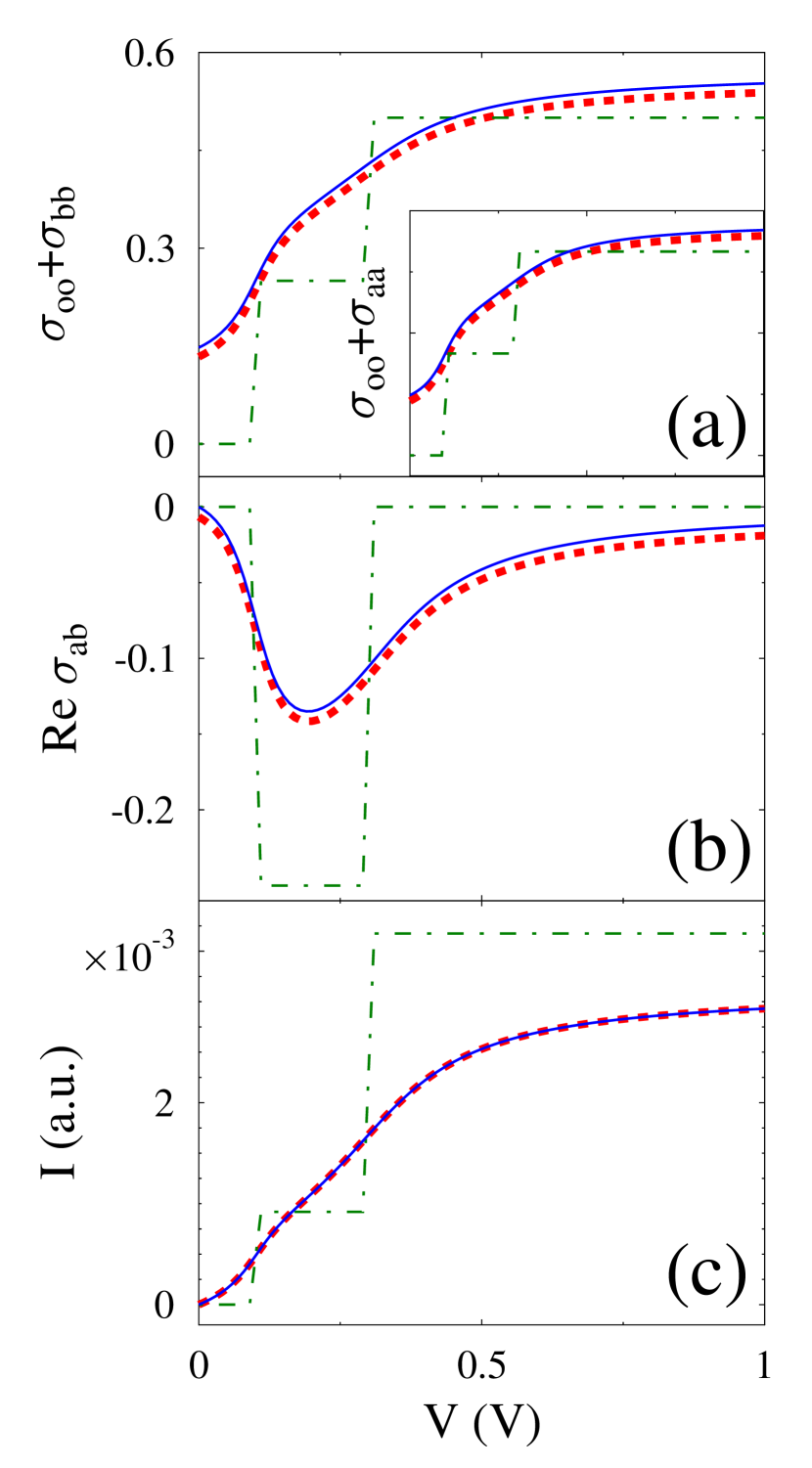
Figure 1: (Color online) Two-level bridge by Redfield QME (dash-dotted line, green), NEGF (dashed line, red), and self-consistent GQME (solid line, red) approaches. Shown are (a) probabilities, (b) coherence, and (c) current vs. bias. Far off-resonant local basis treatment. See text for parameters.

We start our consideration from a simple far off-resonant case, where $\Gamma_{mn}\ll|\varepsilon_{a}-\varepsilon_{b}|$ ($m,n\in\{a,b\}$). Here our consideration is done in a local molecular basis ($t\neq 0$). The parameters of the calculation are the following: level positions $\varepsilon_{a}=0.2$ eV and $\varepsilon_{b}=0.5$ eV, inter-level hopping $t=0.1$, escape rates for both levels into both contacts $\Gamma^{K}_{aa}=\Gamma^{K}_{bb}=0.1$ eV ($K=L,R$), and level mixing due to coupling to the contacts $\Gamma^{K}_{ab}=\Gamma^{K}_{ba}=0.05$ eV. The Fermi energy in the absence of bias is taken as zero, $E_{F}=0$, and the voltage division factor is $1$, i.e. $\mu_{L}=E_{F}+|e|V$ and $\mu_{R}=E_{F}$. The NEGF calculation is performed on an energy grid spanning the range from $-10$ to $10$ eV with step $10^{-4}$ eV. Both the Redfield QME and our scheme are expected to work properly in this region of parameters. Figure 1 compares the results of the Redfield QME and our new scheme to the exact NEGF results for the model. The main graph and the inset in Fig.1a display populations, Eqs. (38) and (39). The real part of the coherence, Eq.(40), is shown in Fig.1b. The imaginary part of the coherence is zero in this case (not shown). As discussed earlier,Esposito and Galperin (2009) the Redfield QME approach misses the information about the broadening of the molecular levels. Our approach accurately recovers this information. Both populations and coherence are well reproduced by our GQME as well as the current-voltage characteristics (see Fig.1c). Qualitatively, the predictions of the Redfield QME approach are also correct here.

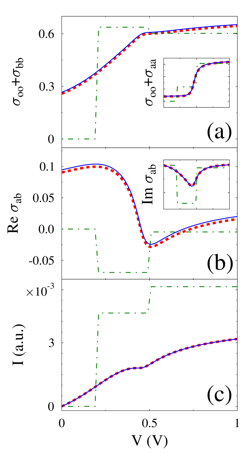
Figure 2: (Color online) Two-level bridge by Redfield QME (dash-dotted line, green), NEGF (dashed line, red), and self-consistent GQME (solid line, red) approaches. Shown are (a) probabilities, (b) coherence, and (c) current vs. bias. Case of strong mixing due to coupling to the contact(s). See text for parameters.

We next consider the case of strong mixing due to coupling to the contact(s). Parameters of the calculation are $t=0$, $\Gamma^{L}_{aa}=0.3$ eV, $\Gamma^{R}_{aa}=0.048$ eV, $\Gamma^{L}_{bb}=0.2$ eV, $\Gamma^{R}_{bb}=0.1125$ eV, $\Gamma^{L}_{ab}=\Gamma^{L}_{ba}=0.12$ eV, and $\Gamma^{R}_{ab}=\Gamma^{R}_{ba}=0.15$ eV. The other parameters are the same as in Fig.1. Figure 2 compares the Redfield QME and our self-consistent GQME scheme with the exact NEGF results. Our scheme still reproduces populations (Fig.2a), coherences (Fig.2b), and current (Fig.2c) accurately. The Redfield QME however fails to reproduce, even qualitatively, the populations (see Fig.2a) and the real part of the coherence (see Fig.2b). This is due to coherence effects through the bath which are not properly captured by the Redfield QME.

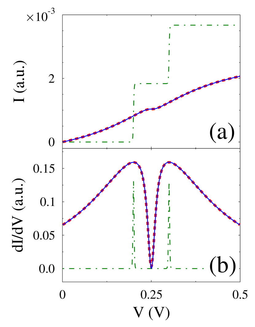
Figure 3: (Color online) Two-level bridge by Redfield QME (dash-dotted line, green), NEGF (dashed line, red), and self-consistent GQME (solid line, red) approaches. Shown are (a) current and (b) conductance vs. bias. Resonant, $\varepsilon_{a}=\varepsilon_{b}$, consideration in a local basis with only level $a$ coupled to contacts, $\Gamma^{K}_{aa}\neq 0$ and $\Gamma^{K}_{bb}=\Gamma^{K}_{ab}=\Gamma^{K}_{ba}=0$ ($K=L,R)$. See text for parameters.

Interference effects in molecular systems were observed experimentally for electron transferC.Patoux et al. (1997) and molecular junction currentsMayor et al. (2003) involving derivatives of benzene connected in meta or para position. They were also extensively discussed in theoretical literature.Stafford et al. (2007); Goldsmith et al. (2007); Solomon et al. (2008a, b, c); Solomon et al. (2009) Figure 3 shows current (a) and conductance (b) vs. bias, for a model system in which destructive interferences can be experimentally observed and which has been discussed earlier in the literature.Solomon et al. (2009) This model is a two-level system with only one of the levels, $a$, attached to both $L$ and $R$ contacts. The other level, $b$, is coupled to the level $a$ through a hopping element $t$. Level $b$ is not directly attached to any contacts. As a result, the tunneling electron has two possible pathways to be transferred from contact $L$ to contact $R$ via the system: one directly through level $a$ and the other by exploring level $b$ on its way. Interference between the two paths leads to destructive interference in the transport characteristics, which reveals itself as a dip in the conductance. Parameters of the calculation are $\varepsilon_{a}=\varepsilon_{b}=0.25$ eV, $t=0.05$ eV, $\Gamma^{L}_{aa}=\Gamma^{R}_{aa}=0.2$ eV and $\Gamma^{K}_{ab}=\Gamma^{K}_{ba}=\Gamma^{K}_{bb}=0$. Fig.3b shows that destructive interference in conductance is accurately captured by our self-consistent GQME approach but not by the Redfield QME.

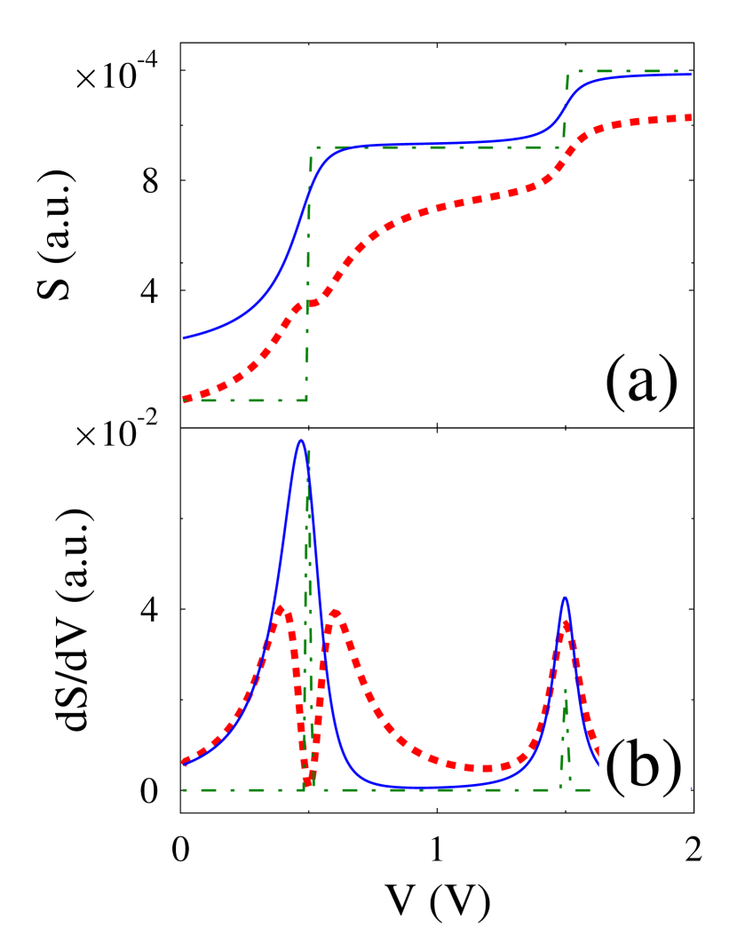
Figure 4: (Color online) Two-level bridge by Redfield QME (dash-dotted line, green), NEGF (dashed line, red), and self-consistent GQME (solid line, red) approaches. Shown are (a) shot noise and (b) differential shot noise vs. bias. See text for parameters.

Finally, we present the results of calculation for the zero-frequency shot noise. The shot noise was calculated using the FCS approach, which for the Redfield QME and our self-consistent scheme yields to expression (34). The FCS within NEGF was discussed in our previous publication.Fransson and Galperin (2010) Note that the FCS for a two-level bridge within QME was also discussed in Ref. Esposito et al., 2007 We intentionally consider two independent levels (no coupling either within the system or through the bath) to demonstrate the general problem that usual QME schemes have in representing higher moments. We assume that the level $\varepsilon_{a}=0.5$ eV is coupled symmetrically to both contacts $\Gamma^{L}_{aa}=\Gamma^{R}_{aa}=0.1$ eV. The other level $\varepsilon_{b}=1.5$ eV is coupled asymmetrically $\Gamma^{L}_{bb}=10\Gamma^{R}_{bb}=0.1$ eV. Other parameters are $t=0$, $\Gamma^{K}_{ab}=\Gamma^{K}_{ba}=0$, and $T=10$ K.

Figure 4 compares the results of the Redfield QME and the self-consistent GQME with the exact results provided by NEGF. It is knownGalperin et al. (2006) that the differential shot noise yields a two-peak structure for a symmetrically coupled molecule, with only a single peak observed for highly asymmetric coupling. One sees that the latter peak (centered around $1.5$ eV in Fig.4b) is reproduced quite well by our self-consistent approach. The double well structure is however missed by both the Redfield QME and our approach (see peak centered aroundi $0.5$ eV). Cumulants beyond first order can be very sensible to approximations and our level of theory, which neglects molecule-contacts correlations beyond second order, has to be improved to properly reproduce them.

Summarizing, within our simple two-level model of molecular junction, the comparison of the proposed self-consistent GQME and the Markovian Redfield QME to the exact results provided by the NEGF shows that the self-consistent GQME is highly accurate even when the Redfield QME fails qualitatively. We find that the self-consistent GQME will only fail in the region of parameters where the inter-level coherence due to the coupling to contacts in the molecular eigenbasis is bigger than the distance between the molecular eigenstates and is of the order of the molecule-contact coupling strength (i.e. exactly at resonance). As a result, in most relevant practical calculations of transport in molecular junctions, we expect our approach to be accurate. The ability of the proposed scheme to treat molecular transport in the language of many-body states of the isolated molecule and its ability to properly account for interference effects makes it a valuable practical tool for ab initio calculations of transport in molecular junctions.

V Conclusion

We present a practical scheme for molecular transport calculation. The scheme is based on a time-local generalized quantum master equation obtained by closing the exact EOM for Hubbard operators by employing a time-reversed evolution ansatz on the Keldysh anti-contour, similar to generalized Kadanoff-Baym ansatz introduced in our previous publication. We note that the approximations involved in derivation of the time-local equation are essentially the same as for the earlier (more traditional) time-nonlocal GQME. The time-locality of the GQME allows us to formulate a feasible self-consistent scheme to calculate the time dependent molecular density matrix and the current in term of molecular many-body states. We find that the convergence of the self consistent method for a simple two-level bridge model is achieved within two iterative steps. The results of the calculation for TLB within self-consistent GQME are compared to Redfield QME approach, and to exact NEGF results. We demonstrate that our scheme (contrary to the usual QME result) properly captures populations and coherences. In particular, destructive interference effects in the molecular devices previously discussed in the literature can now be properly described in the many-body states language, which makes the scheme a valuable tool for practical ab initio calculations. Current-voltage characteristics are reproduced with high accuracy. We are able to calculate the molecular device characteristics in the experimentally relevant regime of low temperatures. We find that the scheme breaks down in the region of the parameters where coherences in the system eigenbasis (i.e. coherences introduced through non-diagonal elements of molecule-contact coupling matrix $\Gamma$) are both bigger than the inter-level separation and are of the order of the escape rates (diagonal elements of the molecule-contact coupling matrix $\Gamma$). Thus, we expect the scheme to be a valuable tool for most practical transport calculations in molecular junctions.

The formulation of a scheme capable of reproducing higher moments of the full counting statistics in the many-body state language that goes beyond the Redfield QME approachEsposito et al. (2009) is the goal of future research.