The Standardized Candle Method for
Type II Plateau Supernovae

Abstract

In this paper we study the “standardized candle method” using a sample of 37 nearby (redshift $z<0.06$) Type II plateau supernovae having $BVRI$ photometry and optical spectroscopy. An analytic procedure is implemented to fit light curves, color curves, and velocity curves. We find that the $V-I$ color toward the end of the plateau can be used to estimate the host-galaxy reddening with a precision of $\sigma(A_{V})=0.2$ mag. The correlation between plateau luminosity and expansion velocity previously reported in the literature is recovered. Using this relation and assuming a standard reddening law ($R_{V}=3.1$), we obtain Hubble diagrams in the $BVI$ bands with dispersions of $\sim$ 0.4 mag. Allowing $R_{V}$ to vary and minimizing the spread in the Hubble diagrams, we obtain a dispersion range of 0.25–0.30 mag, which implies that these objects can deliver relative distances with precisions of 12–14%. The resulting best-fit value of $R_{V}$ is $1.4\pm 0.1$.

1 INTRODUCTION

Core-collapse SNe (CCSNe) are in general closely associated with star-forming regions in late-type galaxies (e.g., Anderson & James, 2008). Therefore, they have been attributed to stars born with initial mass $>$ 8 ${\rm M}_{\odot}$ that undergo the collapse of their iron cores after a few million years of evolution, and the subsequent ejection of their envelopes (e.g., Burrows, 2000). According to theoretical studies, these SNe leave a compact object as a remnant, either a neutron star or a black hole (Baade & Zwicky, 1934; Arnett, 1996; Janka et al., 2007).

Among CCSNe, we can observationally distinguish those with prominent hydrogen lines in their spectra (dubbed Type II; Minkowski, 1941), those with no H but strong He lines (Type Ib), and those lacking H or He lines (Type Ic); see (Filippenko, 1997) and references therein. Although all of these objects are thought to share largely the same explosion mechanism, their different observational properties are explained in terms of how much of their H-rich and He-rich envelopes were retained prior to explosion. When the star explodes with a significant fraction of its initial H-rich envelope intact, it should display a H-rich spectrum and a light curve characterized by an optically thick phase of $\sim$ 100 days of nearly constant luminosity called a “plateau,” which comes to an end at the point when all of the hydrogen in the envelope has recombined. This phase is followed by a sudden drop of 2–3 mag and thereafter by an exponential decay in luminosity caused by the radioactive decay of ⁵⁶Co into ⁵⁶Fe (e.g., Nadyozhin, 2003; Utrobin, 2007). Nearly 50% of all CCSNe belong to this class of “Type II plateau” SNe (SNe IIP; Cappellaro et al., 1999; Botticella et al., 2008).

A decade ago, the standardized luminosities of Type Ia SNe (e.g., Phillips, 1993; Hamuy et al., 1996; Riess et al., 1996; Phillips et al., 1999) led to the construction of Hubble diagrams (HDs) at redshifts $z=0$–0.1 with dispersions of only $\sim 0.15$ mag, which opened up the opportunity to measure the expected deceleration of the Universe. At the end of the millennium, Riess et al. (1998) and Perlmutter et al. (1999) reported independent observations of high-redshift SNe ($z=0.1$–0.5) which permitted the measurement of the expansion history of the Universe over $\sim$ 5 Gyr of lookback time. Contrary to expectations, these observations revealed that the Universe is currently described by an accelerated expansion. The discovery of cosmic acceleration, which was subsequently confirmed by additional studies of SNe Ia (e.g., Astier et al., 2006; Wood-Vasey et al., 2007; Hicken et al., 2009; Freedman et al., 2009), implies the possible existence of a cosmological constant, a concept initially introduced by Albert Einstein at the beginning of the 20th century. Its origin is still a mystery, and there are many other possible candidates for the repulsive “dark energy” that permeates the Universe (see Frieman et al. 2008 for a review).

The acceleration of the Universe has now been indirectly confirmed by other independent experiments such as the Wilkinson Microwave Anisotropy Probe (WMAP; Spergel et al., 2007; Bennett et al., 2003) and baryon acoustic oscillations (BAO; Blake & Glazebrook, 2003; Seo & Eisenstein, 2003), as well as more directly with the integrated Sachs-Wolfe effect (e.g., Boughn & Crittenden, 2004; Fosalba et al., 2003) and X-ray observations of clusters of galaxies (Allen et al., 2008), but it is nevertheless important to obtain additional independent confirmation of the SN Ia results. Although SNe IIP are not as luminous and uniform as SNe Ia, Hamuy & Pinto (2002) showed that the luminosities of the former can be standardized to levels of 0.4 and 0.3 mag in the $V$ and $I$ bands, respectively. This finding converted these objects into precise distance indicators and potentially into useful tools to measure cosmological parameters. Moreover, SNe IIP would be more abundant at high redshift than SNe Ia, since the star-formation rate increases with redshift until $z\approx 2.5$ (see Hopkins & Beacom 2006, and references therein).

Type IIP supernovae provide two routes to distance determinations. First, the “expanding photosphere method” (EPM; Kirshner & Kwan, 1974) is a technique based on theoretical models that is independent of the extragalactic distance scale (Eastman et al., 1996; Dessart & Hillier, 2005). In EPM the spectral energy distribution of the SN is approximated as a black body, and atmosphere models permit one to correct the dilution of the photospheric flux relative to a Planck function due to electron scattering. From a detailed analysis of the properties of the SN atmospheres, Eastman et al. (1996) showed that the most important variable in determining the “dilution factors” is the effective temperature. This result permits one to determine the photospheric angular radius of the SN from a measurement of the color temperature, and infer the distance from the expansion velocity measured from spectral lines, without the need to craft specific models for each SN. This method can achieve dispersions of 0.3 mag in the HD, which translates into a 14% precision in relative distances (Schmidt et al., 1994; Hamuy, 2001; Jones et al., 2009). Another more accurate approach consists of adopting corrections and color temperatures from tailored models for each observation, revealing an accuracy of $\sim$ 10% in distance determination of individual SNe (Dessart & Hillier, 2006; Dessart et al., 2008).

Second, the “standardized candle method” (SCM) is an empirical technique initially proposed by Hamuy & Pinto (2002) based on an observational correlation between the absolute magnitude of the SN and the expansion velocity of the photosphere, the luminosity/expansion-velocity (LEV) relation. This correlation shows that SNe IIP with greater luminosities have higher expansion velocities, which permits one to correct for the large ($\sim$ 4 mag) luminosity differences displayed by these objects to levels of only $\sim 0.3$ mag. So far, the SCM has been applied to 24 low-redshift ($z<0.05$) SNe (Hamuy, 2003b, 2005) and more recently by Poznanski et al. (2009) to 17 low-redshift ($z<0.03$) SNe, as well as by Nugent et al. (2006) to 5 high-redshift ($z<0.29$) SNe. The latter work was the first attempt to derive cosmological parameters from SNe IIP and demonstrated the enormous potential of this class of objects as cosmological probes.

Several major sky-survey programs now in progress or to be deployed in the upcoming years, such as the Palomar Transient Factory (PTF; Rau et al., 2009; Law et al., 2009), the Panoramic Survey Telescope and Rapid Response System (Pan-STARRS; Hodapp et al., 2004), the Large Synoptic Survey Telescope (LSST; Tyson et al., 2003), the Visible and Infrared Survey Telescope (VISTA; Emerson et al., 2004), the VLT Survey Telescope (VST; Capaccioli et al., 2003), the Dark Energy Survey (DES; Castander, 2007), and the SkyMapper (Granlund et al., 2006), offer the promise of discovering SNe by the thousands. Thus, we will be inevitably confronted by enormous amounts of data on SNe IIP which will contain potentially valuable cosmological information. The challenge is to find an implementation of SCM that does not require spectroscopic data since these surveys will be purely photometric.

In spite of the great potential shown by the SCM, it still suffers from a variety of problems which need to be addressed: (1) the lack of a well-defined maximum in the light curves has prevented us from defining the phase of each event; (2) each SN shows a different color evolution, which has compromised the use of the photometric data for the determination of host-galaxy extinction; (3) the assumption for dereddening employed by Hamuy & Pinto (2002), namely that all SNe reach the same asymptotic color toward the end of the plateau phase, has often led to negative extinction corrections, so it still needs to be further tested; and (4) the small sample size used so far, especially the scarcity of SNe in the Hubble flow, has prevented a proper determination of the intrinsic precision of the method.

With these obstacles in mind, we have developed a robust mathematical procedure to fit the light curves, color curves, and velocity curves, in order to obtain a more accurate determination of the relevant parameters required by the SCM (magnitudes, colors, and ejecta velocities), as described in detail in the thesis work of Olivares (2008). Here we apply this technique to 37 SNe IIP in order to construct a HD, evaluate the accuracy of the SCM, and obtain an independent determination of the Hubble constant. Since our sample has several objects in common with the recent EPM analysis of Jones et al. (2009), we perform a comparison between SCM and EPM.

We organize this paper as follows. In § 2 we describe all of our observational material including telescopes, instruments, and surveys involved. The analysis, methodology, and procedures, such as the $A_{\rm G}$, $K$, and $A_{\rm host}$ corrections, are explained in detail in § 3. The dereddening analysis, the HD, the value of the Hubble constant, and the comparison between SCM and EPM distances are addressed in § 4. The final remarks in § 5 provide a discussion about variations of the reddening law for SNe IIP and the possibility of a nonstandard extinction law in the SN host galaxies. We present our conclusions in § 6.

2 OBSERVATIONAL MATERIAL

This work makes use of data obtained in the course of four systematic SN follow-up programs carried out during the years 1986–2003: (1) the Cerro Tololo SN program (1986–1996); (2) the Calán/Tololo SN program (CT, 1990–1993); (3) the Optical and Infrared Supernova Survey (SOIRS, 1999–2000); and (4) the Carnegie Type II Supernova Program (CATS, 2002–2003). As a result of these efforts, photometry and spectroscopy (some infrared but mostly optical) was obtained for nearly 100 SNe of all types, 51 of which belong to the Type II class. Of these 51 SNe II, a subset of 33 objects meets the requirements for this study. Next we describe in general terms the data acquisition and reduction procedures. For more details the reader can refer to M. Hamuy et al. (2010, in preparation).

2.1 Photometric Data

The photometry was acquired with telescopes from Cerro Tololo Inter-American Observatory (CTIO), Las Campanas Observatory (LCO), the European Southern Observatory (ESO) in La Silla, and Steward Observatory (SO). Many different telescopes and intruments were used to generate this dataset as shown in Table 1. In all cases we employed CCD detectors and standard Johnson-Kron-Cousins-Hamuy $UBVRIZ$ filters (Johnson et al., 1966; Cousins, 1971; Hamuy et al., 2001).

The images were processed with IRAF through bias subtraction and flat-fielding. All of them were further processed through the step of galaxy subtraction using template images of the host galaxies. Photometric sequences were established around each SN based on observations of Landolt and Hamuy standards (Landolt, 1992; Hamuy et al., 1992, 1994). The photometry of all SNe was performed differentially with respect to the local sequence on the galaxy-subtracted images. The transformation of instrumental magnitudes to the standard system was done by taking into account a linear color term and a zero point. Although this procedure partially removes the instrument-to-instrument differences in the SN magnitudes, it should be kept in mind that significant systematic discrepancies can still remain owing to the nonstellar nature of the SN spectrum (e.g., Hamuy et al., 1990).

Complementary photometry for SN 2003gd obtained by Van Dyk et al. (2003) and Hendry et al. (2005) was also incorporated in our analysis.

2.2 Spectroscopic Data

The spectroscopic data were also obtained with a great variety of instruments and telescopes, as shown in Table 1. The observations consisted of the SN observation immediately followed by an emission-line comparison lamp taken at the same position in the sky, and 2–3 flux standards per night from the list of Hamuy et al. (1992, 1994). We always used CCD detectors, in combination with different gratings/grisms and blocking filters. The reductions were performed with IRAF and consisted of bias subtraction, flat-fielding, one-dimensional (1D) spectrum extraction and sky subtraction, wavelength calibration, and flux calibration. No attempts were made to remove the telluric lines.

Our spectroscopic database was complemented with spectra obtained by the CfA SN program with the FAST CCD spectrograph (Fabricant et al., 1998) at the 1.5-m telescope of the Whipple Observatory (see Matheson et al. 2008 for details on the data reduction), and by the University of California, Berkeley SN program with the Kast double CCD spectrograph (Miller & Stone, 1993) on the Shane 3-m telescope at Lick Observatory. The above standard procedures, including removal of telluric absorption lines, were employed to reduce the Lick spectra (e.g., Foley et al., 2003).

2.3 Subsample Used for this Work

Of the 51 SNe II observed in the course of these four surveys, a subset of 33 objects comply with the requirements of (1) being a member of the plateau subclass; (2) having sufficient spectroscopic temporal coverage; and (3) having light curves with good temporal coverage. To this sample we added four SNe from the literature: SN 1999gi, SN 2004dj, SN 2004et, and SN 2005cs. Table 2 lists our final sample of 37 SNe IIP. For each SN this table includes the name of the host galaxy, the equatorial coordinates of the SN, the heliocentric redshift and its source, the reddening due to our own Galaxy (Schlegel et al., 1998), and the survey during which the SN was observed.

3 METHODOLOGY AND PROCEDURES

In the thesis work of Olivares (2008), we describe in detail the techniques for correcting the photometry for Galactic absorption ($A_{\rm G}$), $K$-correction terms, and host-galaxy dust absorption ($A_{\rm host}$) — the so-called “$AKA$ corrections”. In brief, we employ a library of 196 spectra of SNe II (including other SN II types than just SNe IIP) to synthesize $K$-terms and absorption coefficients given the specific redshift and $A_{V}$ value of each SN. Synthetic $B-V$ and $V-I$ colors are used as proxies for the spectral energy distribution in order to account for the evolution of each SN.

3.1 Fits to Light, Color, and Velocity Curves

In the first incarnation of the SCM, Hamuy & Pinto (2002) measured all of the relevant quantities (magnitudes, colors, and velocities) at fixed epochs with respect to the time of explosion. In most cases, however, it proves hard to constrain this time, thus hampering the task to compare data obtained for different SNe. It would be ideal to have a conspicuous feature in the light curves; unfortunately, unlike other SN types, SNe IIP generally do not show a well-defined maximum during the plateau phase.

One way around this is to use the end of the plateau as an estimate of the time origin for each event. In practice it is not easy to measure this time owing to the generally coarser sampling of the light curves at this phase. Thus, our first aim is to implement a robust light-curve fitting procedure in order to obtain a reliable time origin to be used as a uniform reference epoch to measure magnitudes, colors, and expansion velocities. In the remainder of this section, we proceed to implement fitting methods to measure reliable colors and expansion velocities.

3.1.1 $BVRI$ Light-Curve Fits

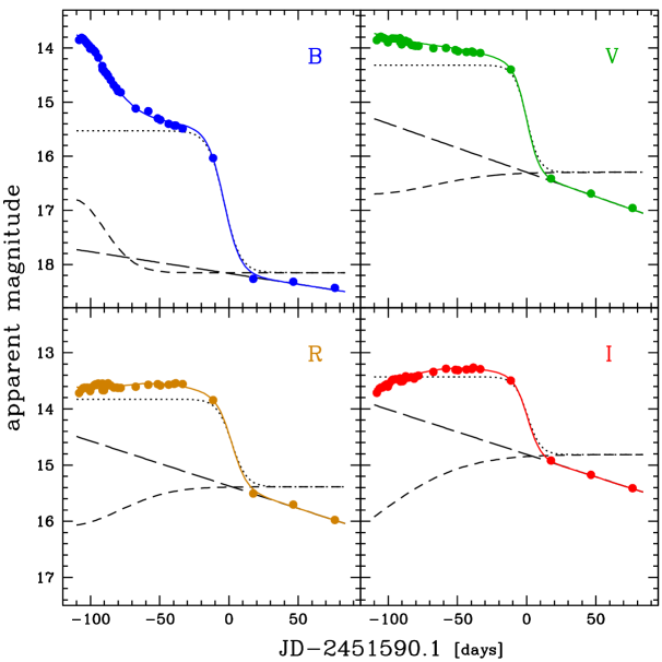
Figure 1: $BVRI$ light curves of SN 1999em. $BVRI$ magnitudes are respectively shown in blue (top-left), green (top-right), brown (bottom-left), and red (bottom-right). The colored solid line corresponds to the analytic fit. The black lines represent the decomposition of the main function into its three components: the Fermi-Dirac function (dotted line), a straight line (long-dashed line), and a Gaussian function (short-dashed line). The origin of the time axis corresponds to $t_{PT}$ in Julian days for SN 1999em. Since the instrumental error bars are smaller than the symbols, they are not shown.

Figure 1 shows the $BVRI$ light curves of SN 1999em. As can be seen, there are three distinguishable phases in the light curves.

—

The plateau phase, in which the SN shows an almost constant luminosity during the first $\sim$ 100 days of its evolution. This phase corresponds to the optically thick period in which a hydrogen recombination wave recedes in mass coordinate, gradually releasing the internal energy of the star (see Kirshner & Kwan 1974; Nadyozhin 2003; Utrobin 2007; Bersten & Hamuy 2009, and references therein).

—

The linear or radioactive tail, a linear decay in magnitude (exponential in flux) starting about 130 days after the explosion. This phase corresponds to the optically thin period powered by the ⁵⁶Co $\rightarrow$ ⁵⁶Fe radioactive decay (e.g., Weaver & Woosley, 1980).

—

A transition phase of $\sim$ 30 days between the plateau and linear phases.

Both the plateau and linear phases are trivial to model if taken separately, but the abrupt transition makes the fitting task much more challenging, especially with coarsely sampled light curves. After considering several options we ended up using the arithmetic sum of the three functions shown in Figure 1, as follows.

(1)

A Fermi-Dirac function (dotted line in Figure 1), which provides a very good description of the transition between the plateau and radioactive phases:

$$f_{\rm FD}(t)=\frac{-a_{0}}{1+e^{(t-t_{\rm PT})/w_{0}}},$$ (1)

where $a_{0}$ represents the height of the step in units of magnitude, $t_{\rm PT}$ corresponds to the middle of the transition phase and is a natural candidate to define the origin of the time axis, and $w_{0}$ quantifies the width of the transition phase. At $t=t_{\rm PT}-3w_{0}$ the height of the step has been reduced by 4.7%, and it decreases down to 95.3% at $t=t_{\rm PT}+3w_{0}$.

(2)

A straight line (long-dashed line in Figure 1) which accounts for the slope due to the radiactive decay:

$$l(t)=p_{0}\,(t-t_{\rm PT})+m_{0},$$ (2)

where $p_{0}$ corresponds to the slope of radioactive tail and an approximate slope for the plateau in units of mag per day, and $m_{0}$ corresponds to the zero point in magnitude at $t=t_{\rm PT}$.

(3)

A Gaussian function (short-dashed line in Figure 1), which serves mainly for fitting the $B$ light-curve bump and the $I$ light-curve curvature during the plateau phase:

$$g(t)=-P\,e^{-\left(\frac{t-Q}{R}\right)^{2}},$$ (3)

where $P$ is the height of the Gaussian peak in units of magnitudes, $Q$ is the center of the Gaussian function in days, and $R$ is the width of the Gaussian function. The Gaussian function is also useful for reproducing the small-scale features that can appear in the $V$-band plateau.

The resulting analytic function we use to model the light curves is the sum of the three functions detailed above,

$$F(t) = f_{\rm FD}(t)+l(t)+g(t)$$ (4)

$$= \frac{-a_{0}}{1+e^{(t-t_{\rm PT})/w_{0}}}+p_{0}\,(t-t_{\rm PT})+m_{0}-P\,e^{-\left(\frac{t-Q}{R}\right)^{2}},$$

which has eight free parameters. This function is fitted to the individual light curves in unison (not by parts) using a $\chi^{2}$ minimizing procedure. In order to find the minimum $\chi^{2}$, we use the Downhill Simplex Method (Nelder & Mead, 1965). Despite being not very efficient in terms of the number of iterations required, it provides robust solutions. Examples of the analytic fits are shown as solid lines in Figure 1. Although we cannot model most of the small-scale features in the plateau, the fitting does a very good job modelling the transition. Furthermore, the analytic function gives us important parameters that characterize the light-curve shape, particularly $t_{\rm PT}$ which provides a time origin. In the plots in Figure 1, the time axis is chosen to coincide with the value of this parameter obtained from the $V$ light curve. In Table 3 we gather the eight parameters and the corresponding reduced $\chi^{2}$ ($\chi_{\nu}^{2}$) of the $V$ light curve fitting for the whole SN sample.

A critical quantity in the analysis that follows is $t_{\rm PT}$ and its uncertainty, both of which determine the uncertainties in all of the relevant SCM quantities. For most cases, when the tail phase has been observed, the $\chi^{2}$ minimizing routine has no difficulties finding $t_{\rm PT}$ and delivers a credible error. On the other hand, when the light curve does not have any late-time data points, the routine underestimates $\sigma(t_{\rm PT})$, in which case we need to provide a more realistic estimate of this uncertainty. Only for a few cases did we have to arbitrarily set $t_{\rm PT}$ and its error based on the light-curve sampling (see Column 3 in Table 3).

Regardless of the sampling of the light curves, we assign a minimum of $\sigma(t_{\rm PT})=2$ days. Although these uncertainties in $t_{\rm PT}$ are very conservative and arbitrary, they do not translate into high or unrealistic errors in quantities such as magnitudes, colors, or expansion velocities, as we will see later.

3.1.2 Color-Curve Fits

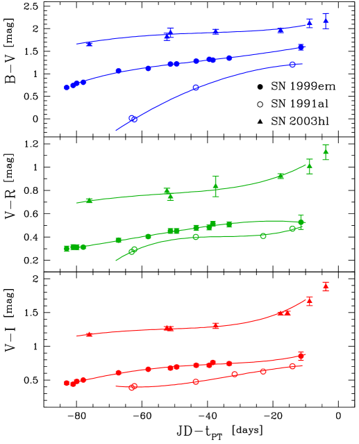
Figure 2: $B-V$, $V-R$, and $V-I$ color curves of SN 1999em (filled circles), SN 1991al (open circles), and SN 2003hl (filled triangles) corrected for the $A_{\rm G}$ and $K$-terms. This comparison demonstrates that each SN displays a different color evolution, precluding the determination of color excesses from a simple color offset after correcting for the $A_{\rm G}$ and $K$-terms. For SN 1991al the error bars are always smaller than the symbols and therefore not plotted.

Figure 2 shows the $B-V$, $V-R$, and $V-I$ colors of three prototypical SNe IIP corrected for $A_{\rm G}$ and $K$-terms as described by Olivares (2008, Chapter 3.1). The time origin in the abscissa corresponds to $t_{\rm PT}$, the middle of the transition phase. In each case we employ all the data points between days $-100$ and $-10$ to fit a Legendre polynomial shown with solid lines in Figure 2. The degree of the polynomial was chosen on a case-by-case basis and varied between third and sixth order. It is evident that, during the plateau phase, the photosphere gets redder with time owing to the decrease of the surface temperature as the SN expands and to a redistribution of flux from blue to red wavelengths due to line blanketing. According to the theory, the photospheric temperature should approach and never get below the temperature of hydrogen recombination around 5000 K. Based on this physical argument, Hamuy & Pinto (2002) argued that all SNe IIP should reach the same intrinsic colors toward the end of the plateau phase; hence, they proposed that the color excesses measured at this phase could be attributed to dust reddening in the SN host galaxy and be exploited to measure $A_{\rm host}$. Hamuy & Pinto (2002) performed their analysis with a simple naked-eye estimate of the asymptotic colors. Here we improve significantly this situation through the formal color-curve fitting procedure described above.

Armed with the polynomial fits, we proceeded to interpolate colors on a continuous grid with one-day spacing between days $-80$ and $-10$ for analyzing colors at multiple epochs (see § 3.2). In a handful of cases, the data did not encompass the whole grid and we had to extrapolate colors, but never by more than 3 days from the nearest data point.

3.1.3 Fe II Based Expansion-Velocity Curves

The third ingredient for SCM is the velocity of the SN ejecta. Different spectral lines yield different expansion velocities depending on the region from which the photon is emitted. The Fe II $\lambda 5169$ line is thought to be a good proxy for SN IIP photospheric velocity (Dessart & Hillier, 2005) and has been previously employed for SCM. Here we use the Fe II expansion velocities measured by Jones et al. (2009) from the minimum of the P-Cygni line profile after correcting the spectra for the heliocentric redshifts of the host galaxies. The uncertainties of these measurements were estimated to be $\sim 85$ km s^-1 from the quality of the wavelength calibration and the signal-to-noise ratio (S/N) of the absorption feature of the P-Cygni line profile. Although these measurements do not consider relativistic corrections, the latter prove negligible ($\lesssim 40$ km s^-1) in the range considered here (2000–5000 km s^-1).

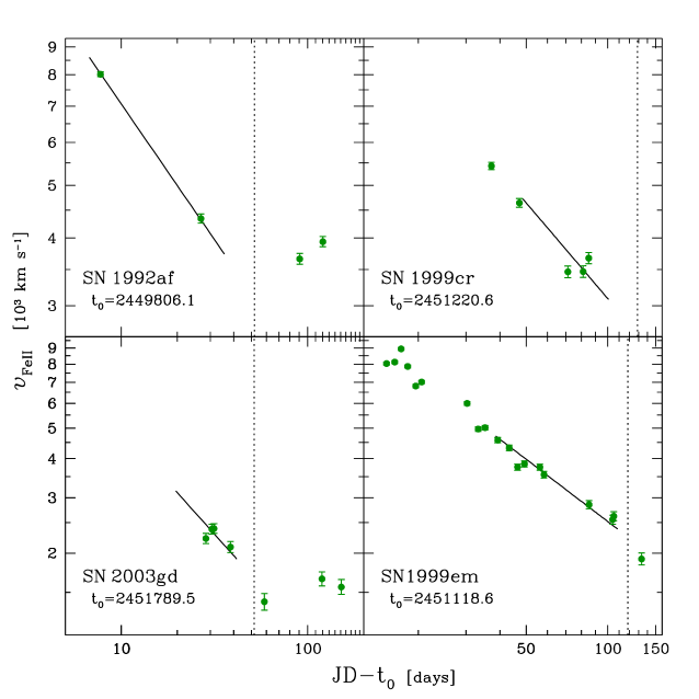
Figure 3: Four expansion velocity curves representative of the SN sample measured by means of the Fe II $\lambda$5169 line profile. While solid lines correspond to a power-law fit (equation 5), dashed lines show the transition time. The $t_{0}$ parameter of the fit was choosen as the time origin due to plotting restrictions. For SN 1992af (top-left panel) we fit only two velocities (see § 3.1.3 for more details). The top-right panel shows a 15-day extrapolation beyond the last data point for SN 1999cr. The bottom-left panel shows a 10-day extrapolation for SN 2003gd prior to the first data point. SN 1999em velocities are shown in the bottom-right panel as an example of good sampling.

Figure 3 shows Fe II velocities as a function of SN phase, for four different SNe selected for their wide range of sampling characteristics. As shown by Hamuy & Pinto (2002), the Fe II $\lambda 5169$ expansion velocity curve during the plateau phase can be properly modeled with a power law, which we choose to be of the form

$$\upsilon_{\rm FeII}(t)=A\,(t-t_{0})^{\alpha},$$ (5)

where $A$, $t_{0}$, and $\alpha$ are free fitting parameters without obvious physical meaning.

In general, we fit for all three parameters, but when only two velocity measurements are available (e.g., SN 1992af in the top-left panel of Figure 3) we fix the $\alpha$ exponent to $-0.5$, which corresponds to a typical value for our sample. As shown with solid lines in Figure 3, the fits are quite satisfactory. Here we choose to restrict the power-law fits to the plateau phase, since the power-law behavior is not observed for expansion velocities beyond the transition phase. We use the same one-day continuous grid as for the color curves in order to interpolate velocities at different epochs between $-80$ and $-10$ days. Given the good quality of the fits and the shallow slope at late epochs, we allow extrapolations of up to 15 days past the nearest data point (see SN 1999cr in Figure 3). At the early-time boundary, we reduce the extrapolations to 10 days prior to the first point, because the power law becomes steeper at early times (e.g., see SN 2003gd in Figure 3). When only two velocity measurements are available we reduce the extrapolations by 5 days. Since at the end of the plateau phase the SN atmosphere starts to become nebular, we discarded data points beyond the transition in the velocity fits. We do not impose any constraints on the first data point.

3.2 Host-Galaxy Extinction Determination

To determine the host-galaxy extinction, we assume that all SNe IIP should evolve from a hot initial stage to one of uniform photospheric temperature, owing to the hydrogen-recombination nature of their photospheres.

Although simple in theory, there are a few practical difficulties when comparing the color evolution. First, it is not always possible to constrain the time of explosion and accurately compare color curves of different objects. One way around this is to use the transition time, $t_{\rm PT}$, defined in § 3.1.1. The second problem is illustrated in Figure 2: the color-curve shapes can vary significantly from one SN to another, preventing one from measuring a single color offset between two SNe. To circumvent this, we pick a single fiducial epoch in the color evolution and assess the performance of the color as a reddening estimator. Our polynomial fits to the color curves are very convenient for this purpose, since they allow us to interpolate reliable colors on a day-to-day basis over a wide range of epochs and explore which epoch gives the best results.

If all SNe share the same intrinsic temperature at some epoch, we expect the subset of dereddened SNe to have nearly identical colors ($C_{0}$); the remaining objects should show color excesses, $E(C)=C-C_{0}$, in direct proportion to their extinctions. A useful diagnostic to check our underlying assumption is the color-color plot: unreddened SNe should occupy a small region in this plane. If we further assume the same extinction law in the SN host galaxies, the subset of extinguished objects should describe a straight line originating from such a region. The figures of merit in this test are (1) the color dispersion displayed by the unreddened SNe, (2) the slope described by the reddened SNe (which is determined by the extinction law), and (3) the dispersion relative to the straight line (the smaller the better).

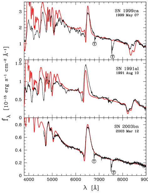
Figure 4: Type IIP SN atmosphere models (wide red line) fitted to our spectra (black line) in the rest frame. The top panel shows an example of an unsatisfactory fit to one of our late-time spectra. The middle panel shows a better fit to an early-time spectrum of SN 1991al. A much better fit is achieved for an early-time spectrum of SN 2003bl as shown in the bottom panel. Strong telluric lines are marked.

We have identified four objects in our sample (SN 2003B, SN 2003bl, SN 2003bn, SN 2003cn) consistent with zero reddening. These objects were selected for having (1) no significant Na I D interstellar lines in their spectra at the redshifts of their host galaxies, and (2) early-time spectra that show no signs of host-galaxy extinction. To judge the latter we used extinction values determined from fits of SN IIP atmosphere models to our early-time spectra as done by Dessart & Hillier (2006) and Dessart et al. (2008). Such models use the SN spectral lines to constrain the photospheric temperature and the continuum to restrict the amount of extinction. Examples of fits are shown in Figure 4.

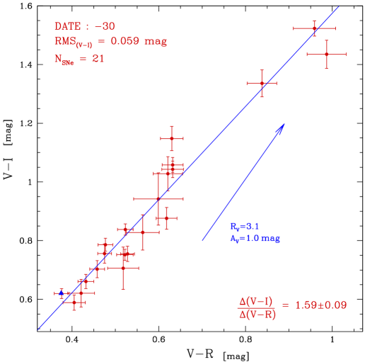
Figure 5: $V-I$ versus $V-R$ diagram for 21 SNe IIP having $VRI$ photometry corrected for the $A_{\rm G}$ and $K$-terms. The blue line is a least-squares fit to the data, with a slope of $1.59\pm 0.09$. The blue arrow has a slope of 2.12 and corresponds to the reddening vector for $A_{V}=1.0$ mag and a standard Galactic extinction law ($R_{V}=3.1$). The blue triangle shows the one SN of this subsample consistent with zero extinction having $R$-band photometry.

We investigated two color-color plots ($V-I$ versus $V-R$, and $V-I$ versus $B-V$) over a wide range of epochs (from day $-50$ to $-15$) after correcting the photometry for Galactic extinction and $K$-terms as described by Olivares (2008). The best results were found for the $V-I$ versus $V-R$ diagram constructed from day $-30$ and shown in Figure 5. Fortunately, all SNe in our sample have enough data to interpolate color curves at day $–30$. At this epoch, approximately the end of the plateau, we obtain the linear behavior expected for a sample with the same intrinsic color but different degrees of extinction. Shown with a triangle is the single SN consistent with zero extinction which is, remarkably, one of the bluest objects in this diagram; the other three unextinguished SNe do not have $R$-band photometry. A least-squares fit to the data yields a slope of $1.59\pm 0.09$, which is lower than the $E(V-I)/E(V-R)=2.12$ ratio expected for a Galactic extinction law ($R_{V}=3.1$) shown as a vector in Figure 5. This suggests a somewhat different extinction law in the SN hosts compared to the Galaxy. The dispersion of 0.059 mag in $V-I$ is a promising result as it translates into an uncertainty of $A_{\rm host}(V)\,=\,0.15$ mag, which corresponds to the limiting precision of this method. The reduced $\chi^{2}$ of 1.55 implies that the dispersion can be accounted almost solely by our error bars and that any instrinsic color dispersion in our sample is $\leq 0.06$ mag. The bottom line is that both the $V-R$ and $V-I$ colors fulfill the minimum requirements as reddening indicators.

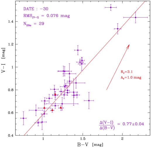
Figure 6: $V-I$ versus $B-V$ diagram for 29 SNe IIP having $BVI$ photometry corrected for the $A_{\rm G}$ and $K$-terms. The red line is a least-squares fit to the data, with a slope of $0.77\pm 0.04$. The red arrow has a slope of 1.38 and corresponds to the reddening vector for $A_{V}=1.0$ mag and a standard Galactic extinction law ($R_{V}=3.1$). The red triangles show the four SNe consistent with zero host-galaxy extinction.

The best results from the $B-V$ versus $V-I$ analysis, obtained from day $-30$, are shown in Figure 6. The four SNe consistent with zero extinction, plotted with triangles, have weighted average colors of $(B-V)_{0}=1.147\pm 0.053$ mag and $(V-I)_{0}=0.656\pm 0.053$ mag, where the dispersion was used as measure of the uncertainty. Note that there are five SNe in this diagram which are slightly bluer than the unreddened sample. The $V-I$ color dispersion of 0.076 mag is greater than that obtained in Figure 5 and is most likely due to the $B-V$ color, since the $B$ band is more sensitive to the metallicity of the SN, owing to many absorption lines that lie in this spectral region. Therefore, we believe that the greater dispersion in this diagram could be due to the different metallicities of our SN sample. A least-squares fit to the data yields a slope of $0.77\pm 0.04$. This slope is quite different from the $E(V-I)/E(B-V)=1.38$ ratio expected for the Galactic extinction law (shown as a vector in Figure 6), in agreement with the departure from a standard reddening law seen in the $V-I$ versus $V-R$ diagram.

We conclude from our exploration that, while the $B-V$ color is problematic, both the $V-R$ and $V-I$ colors offer a promising route for dereddening purposes. In what follows, we will employ solely the $V-I$ color since only a small subset of our objects possess $R$-band photometry. Although the evidence points to a non-Galactic reddening law, for now we will assume a standard reddening law (later we will relax this assumption; see § 4.3.2).

Using our library of SN II spectra, we computed synthetically the appropriate conversion factor between $E(V-I)$ and $A_{V}$ for SNe II and a standard reddening law ($R_{V}=3.1$), yielding

$$\beta_{V}=\frac{A_{V}}{E(V-I)}=2.518.$$ (6)

The host-galaxy extinction can be computed from $A_{V}(V-I)=\beta_{V}\,[(V-I)-(V-I)_{0}]$ and, assuming an intrinsic color of $(V-I)_{0}=0.656\pm 0.053$ mag, its numerical expression with the corresponding uncertainty is

$$A_{V}(V-I) = 2.518\,[(V-I)-0.656],$$ (7)

$$\sigma(A_{V}) = 2.518\,\sqrt{\sigma_{(V-I)}+0.053^{2}+0.059^{2}},$$

where $V-I$ corresponds to the color of a given SN at day $-30$ (corrected for $K$-terms and foreground extinction) and $\sigma_{(V-I)}$ combines the instrumental errors in the $V$ and $I$ magnitudes, the uncertainty in $A_{\rm G}$ and the $K$-terms (see Olivares, 2008, Chapters 3.1.1 and 3.1.2, respectively), and the uncertainty in $t_{\rm PT}$ (§ 3.1.1). The uncertainty in the intrinsic $(V-I)_{0}$ color was also included in the error of $A_{V}$ along with the $V-I$ standard deviation in the $V-I$ versus $V-R$ diagram.

The host-galaxy reddening values obtained from this technique are listed in Column 5 of Table 4 (with the uncertainties given in parentheses for the whole sample of 37 SNe). There are eight SNe with $V-I$ colors bluer than $(V-I)_{0}$ which stand out in this table for their inferred negative reddenings. Although not physically meaningful, these negative values are statistically consistent with zero or moderate reddenings. In fact, seven of these eight objects differ by $<1.1\sigma$ from zero reddening. Only SN 1992af differs by $1.8\sigma$ from $A_{\rm host}=0$ mag.

As a comparison, Krisciunas et al. (2009) employed a similar procedure to determine the extinction to SN 2003hn. While we get $A_{V}=0.46\pm 0.21$, they obtained $A_{V}=0.54\pm 0.14$, values that are consistent within the uncertainties. In the following section we compare this method with other dereddening techniques.

4 ANALYSIS

4.1 Comparing Dereddening Techniques

SN IIP atmosphere models were fitted to our library of spectra as done by Dessart & Hillier (2006) and Dessart et al. (2008). In these fits the spectral lines are used to constrain the photospheric temperature and the corresponding continuum is employed to estimate the extinction. Thus, the quality of the fit depends on (1) the determination of the photospheric temperature by means of the spectral lines, and (2) how well the continuum is represented by the extinguished blackbody emission. A crucial condition for this technique to work is the spectrophotometric quality of the spectra.

In general, our observations were obtained with the slit oriented along the parallactic angle (Filippenko, 1982) and the relative shape of the spectra should be accurate. However, this was not always possible; moreover, sometimes the spectra were contaminated by light from the host galaxy. Accordingly, we first checked the flux calibration of each spectrum by synthesizing magnitudes and comparing them to the observed magnitudes, duly interpolated to the time of the spectroscopy. We typically found an agreement better than 0.05 mag between the observed and synthetic colors, thus confirming our confidence in the flux calibration. In the 64 cases (18% of all spectra) where we found significant differences between synthetic and observed colors ($\geq$ 0.1 mag for any color), we applied a low-order polynomial correction to the spectrum. Basically, this “mangling” correction used the observed photometry to change the slope of a spectrum. After checking the flux calibration (and mangling it, if needed), the next step was to correct for Galactic absorption and deredshift the spectra. This database was then used for the atmosphere model fits. Examples of the fits are shown in Figure 4.

The resulting spectroscopic reddenings are summarized in Column 2 of Table 4. As pointed out by Dessart & Hillier (2006), the spectrum-fitting technique works much better with early-time spectra than with late-time observations. At late times the photosphere has receded in mass, exposing inner and more metal-rich layers, which translates into an overabundance of heavy-element absorption lines. Therefore, the fitting to the continuum (essentially a temperature fitting) is hampered by the increased line opacity at late times. We thus divided our sample into four subcategories based on the epoch and the flux quality of the spectra used in the reddening determination: (a) gold: early-time spectra, without mangling correction; (b) silver: early-time spectra, with mangling correction; (c) bronze: late-time spectra, without mangling correction; and (d) coal: late-time spectra, with mangling correction. Note that the main criterion is whether the spectrum was obtained at early or late times, and the second criterion corresponds to the flux-calibration quality. We consider the unmangled spectra to be of higher quality than the mangled ones, because the former do not require any corrections and suggest that the observations were better performed.

The above subclassification is given for each SN in Column 3 of Table 4. Note that the uncertainty is directly related to this subclassification. Dessart et al. (2008) estimate an error of $\sigma_{E(B-V)}=0.05$ mag when using early-time spectra, and $\sigma_{E(B-V)}=0.10$ mag when using late-time spectra. We refine this argument, ramping up from 0.05 to 0.10 mag, depending on the number of spectra employed for each extinction determination. These values are given in Table 4 in units of $A_{V}=3.1\,E(B-V)$.

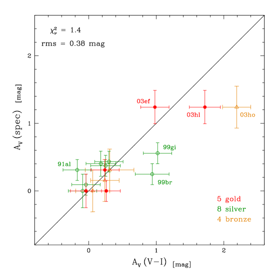
Figure 7: Comparison between two dereddening techniques via $A_{V}$ (mag): the spectrum-fitting method (ordinate) and our technique (abscissa; § 3.2). The figure shows three subclasses defined by the quality of the spectroscopic data used: the gold, silver, and bronze samples (see § 4.1). The solid black line is fixed to show a slope of unity.

Figure 7 shows a comparison between the spectroscopic reddenings $A_{V}$(spec) and our color reddenings $A_{V}(V-I)$ derived in § 3.2, for the 17 SNe belonging to the top three subclasses (gold + silver + bronze). Good agreement is found between both techniques, with a dispersion of 0.38 mag. The resulting $\chi_{\nu}^{2}=1.4$ suggests that this dispersion is consistent with the combined errors of both techniques. The exceptions are two objects, SN 1999br and SN 2003ho. SN 1999br has only plateau-phase photometry, making it hard to determine $t_{\rm PT}$. Although the uncertainty in $t_{\rm PT}$ is quite large (20 days), this does not have a great impact on the error of the $V-I$ color due to the flatness of the color curve at these epochs (+0.0024 mag per day). Another possible reason for the disagreement could be an intrinsically redder $V-I$ color than that of the bulk of the SNe, caused by the extreme properties (low luminosity and expansion velocity) of SN 1999br. The second discrepant object (SN 2003ho) belongs to the bronze group, so it is possible that the difference could be due to the use of a late-time spectrum in the determination of the spectroscopic reddening.

Another way to estimate host-galaxy reddening is from the Na I D $\lambda\lambda$5889, 5896 interstellar absorption doublet observed in the SN spectrum at the host-galaxy redshift. Whenever the line was detected we measured its equivalent width; in those cases where we did not detect the Na I D line we assigned it a null value. In all cases we estimated the uncertainty in the equivalent width (EW) based on the S/N of the continuum around this line. We converted these measurements into visual extinctions, $A_{V}$(Na I D), using the calibration of Barbon et al. (1990):

$$E(B-V)\,\approx\,0.25\,{\rm EW}(\mbox{{Na~{}I}~{}D}),$$ (8)

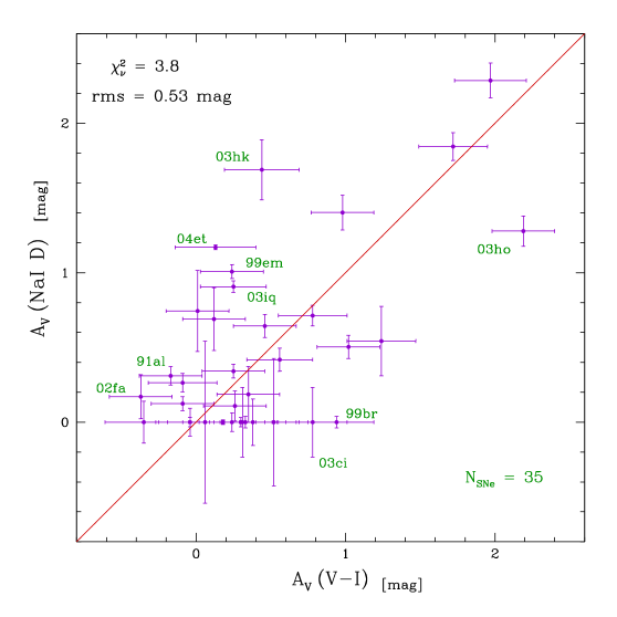
Figure 8: Comparison between two dereddening techniques via $A_{V}$ (mag): the Na I D interstellar line (ordinate) and our technique (abscissa; § 3.2). In each case, the equivalent width of the Na I D interstellar line is transformed into a visual extinction according to the calibration given by Barbon et al. (1990).

where the units of $E(B-V)$ and EW are mag and Å, respectively. Although Turatto et al. (2003) showed that this relation is bimodal, and Blondin et al. (2009) found that the $E(B-V)$ estimates based on EW(Na I D) were highly inaccurate, the $E(B-V)$ values derived from Equation 8 (tabulated in Column 4 of Table 4) provide a rough estimate of $E(B-V)$ to compare with our results. The comparison between $A_{V}$(Na I D) and our technique, shown in Figure 8, exhibits a dispersion of 0.53 mag ($\chi_{\nu}^{2}=3.8$), which is much higher than the $\sigma=0.38$ mag obtained from the previous comparison. The disagreement can be attributed to the fact that the absorption line traces the gas content along the line of sight, but does not necessarily probe dust (Munari & Zwitter, 1997). Furthermore, reddenings derived from the EW of the Na I D lines measured from our low-dispersion spectra simply cannot be expected to be accurate; the D lines produced by a typical interstellar cloud are saturated (Hobbs, 1974). The only way that one can hope to derive a reliable reddening from the D lines is via very high-dispersion spectra that resolve the lines and allow the column density to be determined.

4.2 Luminosity versus Expansion Velocity

After developing the dereddening method based on late-time colors, we can now revisit the LEV relation originally discovered by Hamuy & Pinto (2002), which is at the core of the SCM. For this purpose we applied $AKA$ corrections to our photometry (Olivares, 2008, Chapter 3.1), we used our analytic fits (§ 3.1.1) to interpolate $BVI$ magnitudes on day $-30$, and we employed the cosmic microwave background (CMB) redshifts in Table 5 to convert apparent magnitudes to absolute values (assuming $H_{0}=70$ km s^-1 Mpc^-1 from our final result). In order to assess the dereddening technique, we preserved the relative reddening estimations by keeping the negative values of host-galaxy absorption. We performed a power-law fit to interpolate a velocity contemporaneous with the photometry (day $-30$) as described in § 3.1.1. Only for SN 1999cr did we have to use an extrapolated velocity (see top-right panel in Figure 3). From our original sample of 37 SNe IIP we were able to use 30 SNe to build this relation, since five of them do not have measured Fe II velocities at day $-30$, and two others have extremely low redshifts ($cz_{\rm CMB}<300$ km s^-1).

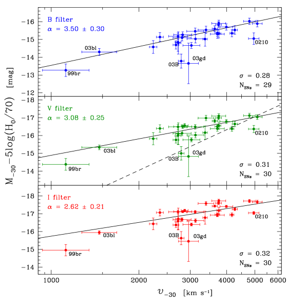
Figure 9: $BVI$-band absolute magnitudes (ordinate) against the Fe II expansion velocity (abscissa) for 29–30 SNe. We use magnitudes corrected for Galactic extinction, $K$-terms, and host-galaxy extinction together with a value of the Hubble constant of 70 km s^-1 Mpc^-1. The dashed line in the middle panel represents the LEV relation for the $V$ band found by Hamuy & Pinto (2002), obtained from magnitudes and velocities measured at day 50 past the explosion (approximately day $-60$ on our own time scale).

Figure 9 shows the resulting LEV relation (absolute magnitude versus expansion velocity) for all $BVI$ bands. Evidently we recover the result of Hamuy & Pinto (2002), namely that the most luminous SNe have greater expansion velocities. In their case the data were modeled with a linear function. Our sample suggests that the relation may be quadratic, but we need more SNe at low expansion velocities to confirm this suspicion. Linear least-squares fits to our $BVI$ data yield the following solutions:

$$M(B)_{-30}-5\,{\rm log}{(H_{0}/70)} = 3.50(\pm 0.30)~{}\log{\Bigr{[}\upsilon_{\rm FeII}(-30)/5000\Bigr{]}}-16.01(\pm 0.20),$$ (9)

$$M(V)_{-30}-5\,{\rm log}{(H_{0}/70)} = 3.08(\pm 0.25)~{}\log{\Bigr{[}\upsilon_{\rm FeII}(-30)/5000\Bigr{]}}-17.06(\pm 0.14),$$ (10)

$$M(I)_{-30}-5\,{\rm log}{(H_{0}/70)} = 2.62(\pm 0.21)~{}\log{\Bigr{[}\upsilon_{\rm FeII}(-30)/5000\Bigr{]}}-17.61(\pm 0.10),$$ (11)

which are shown with solid lines in Figure 9. The relation found by Hamuy & Pinto (2002) for the $V$ band is indicated with the dashed line in the middle panel of the same figure. Given that the study of Hamuy & Pinto (2002) was performed using data at day 50 after explosion (around day $-60$ on our time scale), it is not unexpected that their LEV relation is shifted to higher expansion velocities. Some of the difference in slope is explained by the inclusion of SN 2003bl in our sample, which flattens the correlation. This relation exhibits a dispersion of 0.3 mag, similar to that reported before. Such low scatter is very encouraging as it implies that the expansion velocities can be used to predict the SN luminosities, to standardize them, and to derive distances.

Recently, Kasen & Woosley (2009) have computed hydrodynamical models for SNe IIP, which support the LEV relation initially reported by Hamuy & Pinto (2002). Also, M. Bersten (2010, in preparation) has used her own hydrodynamical models to investigate the LEV relationship. By varying the explosion energy, she has obtained an LEV relation with a slope consistent with that reported here.

4.3 Hubble Diagrams

In order to assess the performance of the SCM, we employ (a) host-galaxy redshifts in the CMB frame with an uncertainty of 187 km s^-1, (b) $BVI$ apparent magnitudes and $V-I$ colors corrected for $K$-terms and Galactic reddening, and (c) Fe II velocities (in units of km s^-1). Table 5 lists these values for the 37 SNe of our sample, of which 35 meet an initial requirement of $cz_{\rm CMB}>300$ km s^-1. The weighted dispersion of the data points around a linear fit in the HDs allows us to evaluate the precision of different approaches.

4.3.1 Using $A_{V}(V-I)$ and $A_{V}$(spec)

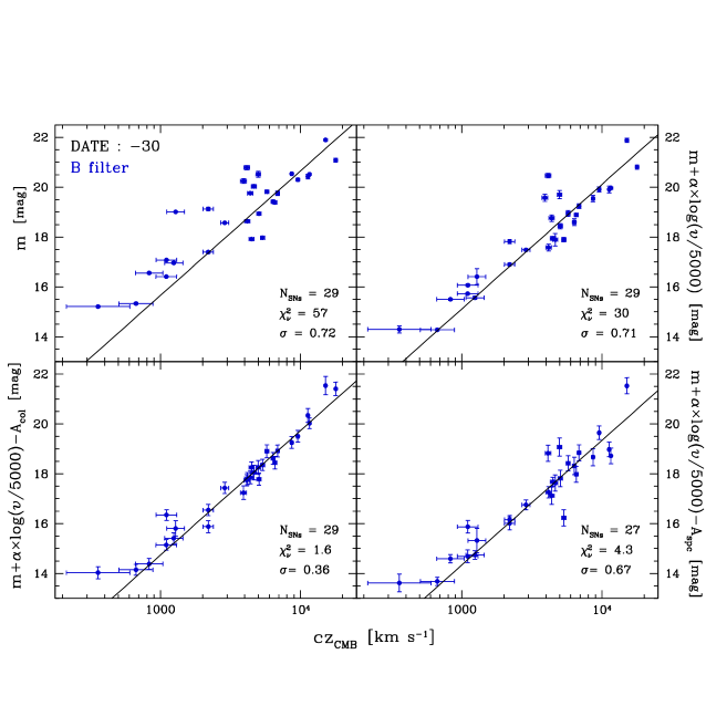
Figure 10: $B$-band Hubble diagrams. The top-left panel shows magnitudes interpolated to day $-30$ previously corrected for Galactic extinction and $K$-terms; the top-right panel shows magnitudes additionally corrected for expansion velocities; the bottom-left panel includes further corrections for color-based host-galaxy extinction (using the $V-I$ color calibration given in § 3.2); and the bottom-right panel replaces the color-based extinction for the spectroscopic reddenings. The horizontal bars in each panel correspond to an adopted uncertainty of 187 km s^-1 in the CMB redshift.

The top-left panel of Figure 10 shows a HD constructed from $B$-band magnitudes interpolated to day $-30$. The top-right panel shows magnitudes additionally corrected for the LEV relation, and the bottom-left panel includes further corrections for host-galaxy extinction (using the $V-I$ color calibration given in § 3.2). In each case we perform a weighted linear least-squares fit of the form

$$m~{}+~{}\alpha\,\log{(\upsilon_{\rm FeII}/5000)}~{}-~{}A_{\rm host}~{}=~{}5\,\log{cz}~{}+~{}zp,$$ (12)

where $m$ is the apparent magnitude corrected for $K$-terms and Galactic absorption, $\upsilon_{\rm FeII}$ is the expansion velocity, $A_{\rm host}$ is the host-galaxy absorption, and $z$ is the CMB redshift. Note that the SN redshift enters logarithmically in this model, implying that low-redshift SNe carry less weight in the fit. The only fitting parameters are $\alpha$ and the zero point ($zp$), but in the top-left panel we set $\alpha=0$ and we fit only for the $zp$. The significant decrease in the dispersion, from 0.72 to 0.36 mag, clearly demonstrates the need to add the velocity and host-galaxy extinction terms.

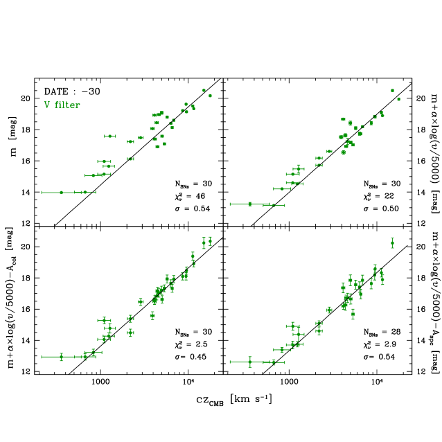
Figure 11: $V$-band Hubble diagrams. The top-left panel shows magnitudes interpolated to day $-30$ previously corrected for Galactic extinction and $K$-terms; the top-right panel shows magnitudes additionally corrected for expansion velocities; the bottom-left panel includes further corrections for color-based host-galaxy extinction (using the $V-I$ color calibration given in § 3.2); and the bottom-right panel replaces the color-based extinction for the spectroscopic reddenings. The horizontal bars in each panel correspond to an adopted uncertainty of 187 km s^-1 in the CMB redshift.

An inspection of the $V$-band diagram (Figure 11) shows a large scatter of 0.54 mag in the top-left panel. When we correct for expansion velocities, the scatter drops to 0.50 mag. This is certainly not unexpected given the LEV relation reported in the previous section. It is encouraging to notice that the dispersion drops from 0.50 to 0.45 mag when we include our host-galaxy extinction corrections; this indicates the utility of our color-based dereddening technique. The reduced $\chi^{2}$ value of 2.45 implies that most of the scatter is caused by the observational errors. We performed the same analysis using other epochs and found that day $-30$ yielded the lowest dispersion.

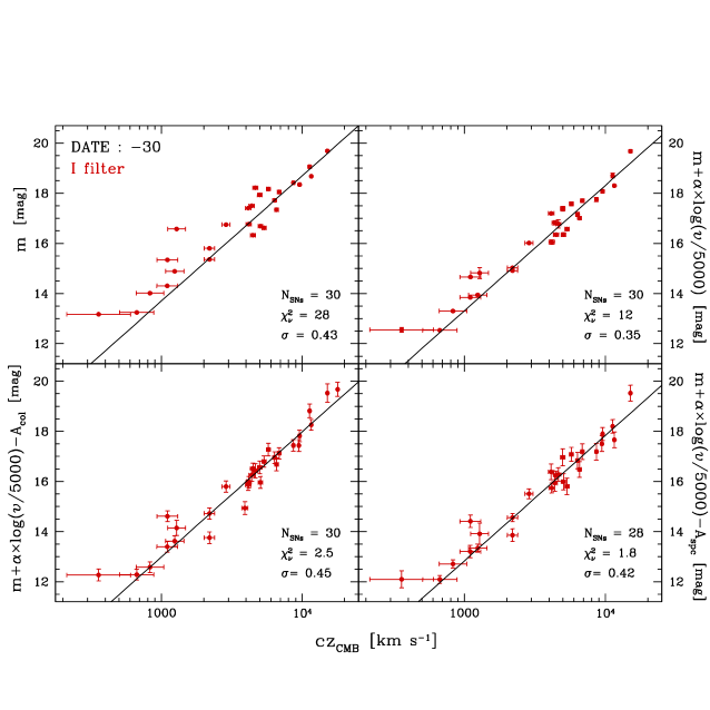
Figure 12: $I$-band Hubble diagrams. The top-left panel shows magnitudes interpolated to day $-30$ previously corrected for Galactic extinction and $K$-terms; the top-right panel shows magnitudes additionally corrected for expansion velocities; the bottom-left panel includes further corrections for color-based host-galaxy extinction (using the $V-I$ color calibration given in § 3.2); and the bottom-right panel replaces the color-based extinction for the spectroscopic reddenings. The horizontal bars in each panel correspond to an adopted uncertainty of 187 km s^-1 in the CMB redshift.

If we turn our attention to the $I$ band (Figure 12), the final dispersion is 0.45 mag, identical to that found in the $V$ band. It seems that the dispersion could have some dependence on wavelength, since it decreases from 0.45 in $VI$ to 0.36 mag in $B$. The scatter of $\sim$ 0.4 mag in $BVI$ is comparable to, but somewhat larger than, the $\sim$ 0.34 mag dispersion obtained in previous SCM studies (Hamuy & Pinto, 2002; Hamuy, 2003b, 2005). It is important to notice that the dispersions are independent of the intrinsic $(V-I)_{0}$ color calculated in § 3.2.

In the bottom-right panels of Figures 10, 11, and 12 we examine the SCM using the spectroscopic reddenings determined for a set of 28 SNe IIP from Table 4 instead of our color-based extinctions. The resulting dispersions in $BVI$ are (0.67, 0.54, 0.42 mag), compared with (0.36, 0.45, 0.45 mag) when using color-based extinctions. All of the fitting parameters derived from both dereddening techniques are compiled in Table 6.

4.3.2 Leaving $R_{V}$ as a Free Parameter

The previous analysis suggests that the dispersions are somewhat larger than the observational errors. One possible source of scatter could be the reddening law. As shown in § 3.2 and Figure 5, we have evidence for a somewhat different extinction law in the SN hosts compared to the Galaxy. Here we take this idea a step further and analyze the HD leaving $R_{V}$ as a free parameter. To accomplish this we model the data with the expression

$$m+\alpha\,\log{(\upsilon_{\rm FeII}/5000)}-\beta(V-I)~{}=~{}5\,\log{cz}+zp.$$ (13)

Note that we are replacing $A_{\rm host}$ in Equation (12) with the term $\beta(V-I)$. The $\beta$ factor is a new free parameter to be marginalized along with $\alpha$ and $zp$, and $V-I$ is the color on day $-30$ uncorrected for host-galaxy dust absorption. This is the same approach adopted by Tripp (1998) for SNe Ia but using decline rate instead of expansion photospheric velocity. The underlying assumption in our case is that the absolute magnitudes of SNe IIP are a two-family function of Fe II expansion velocity and $V-I$ color. The latter is interpreted as a color excess which varies according to dust in the host galaxy. Once $\beta$ is known we can use it to solve for host-galaxy extinction from $A(\lambda)=\beta\,\Bigl{[}\,(V-I)-0.656\,\Bigr{]}$, where 0.656 is the intrinsic $V-I$ color of SNe IIP (see Equations (6) and (7) in § 3.2).

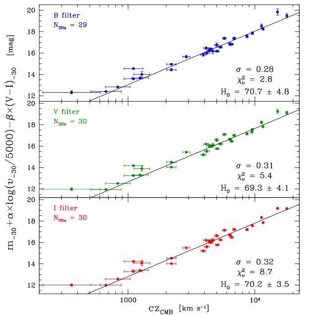
Figure 13: $BVI$ Hubble diagrams leaving $R_{V}$ as a free parameter. In the top, middle, and bottom panels we show the HDs using $BVI$-band magnitudes of 29, 30, and 30 SNe, respectively. The horizontal bars in each panel correspond to an adopted uncertainty of 187 km s^-1 in the CMB redshift.

Figure 13 shows the $BVI$ HDs for our set of 30 SNe IIP. We obtain dispersions of (0.28, 0.31, 0.32 mag) in $BVI$, respectively, compared with (0.36, 0.45, 0.45 mag) when $R_{V}$ is kept fixed. The $\chi_{\nu}^{2}$ values increase from (1.6, 2.5, 2.5) to (2.8, 5.4, 8.7). This change is due to the fact that we are not using the intrinsic color, which gives the major contribution to the errors, even more in the $I$ band. Although we expect a reduction in the scatter due to the inclusion of an additional parameter, the large drop in the dispersion is remarkable. The last three lines of Table 6 show the parameters we obtain by minimizing the dispersion in the HD for each band. When we restrict the sample to objects with $cz_{\rm CMB}>3000$ km s^-1 (leaving aside SNe with potentially greater peculiar velocities), we end up with 19 SNe in the $B$ band and 20 SNe in the $VI$ bands. The resulting HDs in $BVI$ show dispersions of (0.25, 0.28, 0.30 mag), respectively, and the zero points of the HDs change by only 0.02 mag. Not surprisingly, these are lower than the (0.28, 0.31, 0.32 mag) dispersions obtained from the whole sample.

Efforts to remove the peculiar velocities of low-redshift galaxies were made by means of the parametric model for peculiar flows of Tonry et al. (2000). The ingredients of this model are (1) the observed recession velocity of the galaxy, (2) the Hubble constant, and (3) the surface-brightness-fluctuations distance from Tonry et al. (2001). The output is an estimate of the peculiar velocity of the galaxy (see Hamuy, 2003a, § 1.4 for details). After correcting 10 host galaxies in our sample, the results are not conclusive. The scatter in the HDs decreased only 0.01 mag for the $I$ band.

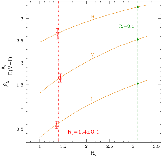
Figure 14: $R_{V}$ versus $\beta$. The solid lines are computed from our library of SN II spectra for each of the $BVI$ bands. The $\beta$ parameters derived from the Hubble diagrams in Figure 13 are shown with red open circles for each of the $BVI$ bands. The red dotted line shows the $R_{V}$-weighted mean for the $BVI$ values of $\beta$. The values for the standard Galactic extinction law are also shown with green dots.

Our assumption is that the term $\beta(V-I)$ in Equation (13) corresponds to the extinction in a broad-band magnitude (with central wavelength $\lambda$). Thus, $\beta$ is the ratio $A(\lambda)/E(V-I)$ (see Equation (6) in § 3.2) and is related to the shape of the extinction law. For each of the $BVI$ bands, we used our library of SN II spectra to compute synthetically the value of $\beta_{\lambda}$ as a function of $R_{V}=A_{V}/E(B-V)$; see Figure 14. This allowed us to convert the $\beta_{\lambda}$ values resulting from our fits into $R_{V}$ values. Our fits yield $\beta_{\lambda}=(2.67\pm 0.13,1.67\pm 0.10,0.60\pm 0.09)$ for the $BVI$ bands, respectively, which translate into $R_{V}=(1.38^{+0.27}_{-0.24},1.44^{+0.13}_{-0.14},1.36^{+0.11}_{-0.12})$. These values are remarkably consistent with each other and significantly lower than the $R_{V}=3.1$ value of the standard reddening law. Independent evidence for a low-$R_{V}$ law has already been reported from studies of SNe Ia (see § 5).

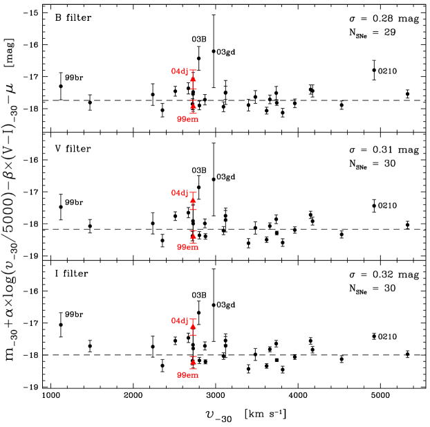
Figure 15: $BVI$-corrected absolute magnitudes (ordinate) against the Fe II expansion velocity (abscissa) for 29–30 SNe (black dots). We use the $H_{0}$ values of Table 7 and the CMB redshifts to compute the distance moduli. The dashed lines show the mean corrected absolute magnitude for the black data points. The red triangles are the two calibrating SNe, whose corrected absolute magnitudes were calculated using their Cepheid distances (see Table 7). Note that, as expected, the two calibrating SNe fall on each side of the corrected absolute magnitude distributions.

The dispersion of 0.28–0.32 mag in the HDs translates into a precision of 13–14% in the determination of relative distances. However, as noticed after inspection of Figure 15, the magnitude residuals are highly correlated among $BVI$ and generally decrease with increasing redshift. The likely explanation is that we are seeing the effects of peculiar velocities of the host galaxies, in which case the precision of the SCM could be better than the 13–14% derived from the scatter in the HDs. To examine this point, for each SN we took the $cz_{\rm CMB}$ values from Table 5, and calculated the distance modulus residual

$$\Delta\mu=m+\alpha\,\log{(\upsilon_{\rm FeII}/5000)}-\beta(V-I)-5\,\log{cz}-zp,$$ (14)

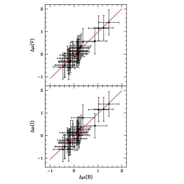
Figure 16: Residuals from the $BVI$ HDs. The correlation between the $V$-filter and $I$-filter residuals against the $B$-filter residuals is shown in the upper and lower panels, respectively. The red lines represent the fit from which the scatter is measured.

for all $BVI$ bands. Figure 16 shows strong correlations of these magnitude differences against each other. The root-mean square (rms) scatter in the $\Delta\mu(B)$ vs. $\Delta\mu(V)$ relation is 0.12 mag, and for $\Delta\mu(B)$ vs. $\Delta\mu(I)$ it is 0.19 mag. This translates to 6% and 9% in distance, respectively. If this correlation of the residuals is due to peculiar velocities, then the true distance precision of SCM is 6–9%, and not 13–14% as derived from the Hubble diagrams (which include scatter produced by the peculiar velocities). This result is very close to the $\sim$ 7–10% precision of methods using SNe Ia (e.g., Phillips, 1993; Hamuy et al., 1996; Riess et al., 1996; Phillips et al., 1999) when they were first used to reveal the acceleration of the Universe, which demonstrates that SNe IIP have great potential for determining extragalactic distances and therefore cosmological parameters.

4.4 The Hubble Constant

The Hubble constant is a parameter of central importance in cosmology which can be determined from our HDs. This can be accomplished as long as we can convert apparent magnitudes into distances. The calibration was done with two objects for which we found Cepheid distances in the literature: SN 1999em ($\mu=30.34\pm 0.19$ mag; Leonard et al., 2002a) and SN 2004dj ($\mu=27.48\pm 0.24$ mag; Freedman et al., 2001). For each calibrating SN we can solve for $H_{0}$ using the expression

$$\log\,H_{0}~{}=~{}0.2~{}\Bigl{[}\,m+\alpha\,\log{(\upsilon_{\rm FeII}/5000)}-\beta(V-I)-\mu-zp+25\,\Bigr{]}_{t=-30},$$ (15)

where $m$ is the apparent magnitude, $\upsilon_{\rm FeII}$ is the expansion velocity, and $V-I$ is the color of the calibrating SN, all measured on day $-30$ and given in Table 5; $\alpha$, $\beta$, and $zp$ are the fitting parameters given in the bottom three lines of Table 6.

Table 7 summarizes our calculations for the two calibrators. We see that the corrected $BVI$ absolute magnitudes of SN 1999em and SN 2004dj differ from each other by 0.86–1.13 mag. This is considerably greater than the scatter of 0.3 mag in the LEV relation, but statistically not impossible; see Figure 15, where we plot with triangles the corrected absolute magnitudes of the two calibrating SNe, on top of the whole sample of SNe employed in the HDs. This difference leads to $H_{0}$ values in the range 62–105 km s^-1 Mpc^-1. With only two calibrating SNe, the SCM still has much room for delivering a more accurate and precise value for $H_{0}$.

4.5 Distances

We are in a position to calculate distances to all of the SNe of our sample. This can be done with the expression

$$\mu=m+\alpha\,\log{(\upsilon_{\rm FeII}/5000)}-\beta(V-I)-\langle M_{\rm corr}\rangle,$$ (16)

where $\langle M_{\rm corr}\rangle$ is the corrected absolute magnitude of SNe IIP on day $-30$. For this purpose we employ the weighted mean of the two calibrating SNe given in Table 7. The resulting values are given in Table 8 for 32 SNe IIP; the last column shows the weighted average of their distance moduli and its uncertainty, assuming no covariance. As Equation 16 shows, it is straightforward to shift the resulting distance moduli to accommodate a new value for $\langle M_{\rm corr}\rangle$. Unfortunately, we are not able to estimate expansion velocities for five objects, and consequently not their distances as well.

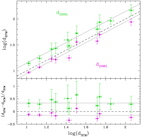
Figure 17: Direct comparison between SCM and EPM distances in Mpc calculated by Jones et al. (2009). In magenta are shown the EPM distances computed from the atmosphere models of E96, while the green triangles are EPM distances obtained from the D05 models. The bottom panel shows the fractional differences between both techniques against $\log(d_{\rm SCM})$. In both panels the dotted lines trace the systematic shifts of the EPM distances with respect to the SCM distances, $\sim$ 40% and $\sim$ 12% using D05 and E96 atmosphere models, respectively. The dashed line in the top panel is fixed to show a slope of unity.

As mentioned in § 1, we can evaluate the accuracy of the SCM from a comparison with EPM distances. For this purpose we employ EPM distances recently calculated by Jones et al. (2009), which are summarized in Table 9 along with our distances for the 11 objects in common between SCM and EPM. Jones et al. (2009) determine EPM distances with two different sets of atmosphere models, both developed based on an analytic approach to calculate dilution factors as a function of a color temperature in order to correct the assumed blackbody emission. Their EPM distances were derived from average dilution factors and not from specific models for each supernova. The EPM distances obtained using the models of Eastman et al. (1996) (E96; Column 2) are $12\pm 5$% shorter than our SCM distances. On the other hand, the EPM distances determined using the models of Dessart & Hillier (2005) (D05; Column 3) are $40\pm 10$% greater than our SCM distances. Both percentage shifts are calculated weighted by the uncertainty in the EPM and SCM distances. These systematic differences can be seen in the top panel of Figure 17, and more clearly in the fractional differences $(d_{\rm EPM}-d_{\rm SCM})/d_{\rm SCM}$ plotted in the bottom panel.

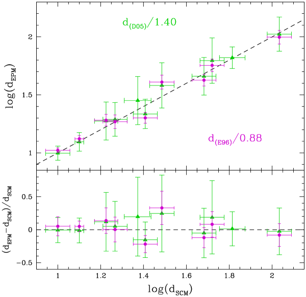
Figure 18: Similar to Figure 17, after removing systematic differences by bringing the EPM distances to the SCM scale (all in Mpc). Only random differences between EPM and SCM distances remain. For the E96 case the discrepancies have a spread of 16%, while for the D05 case the scatter is 13%. The dashed line in the top panel is fixed to show a slope of unity.

The systematic differences among the two sets of EPM distances can be solely attributed to the atmosphere models of E96 and D05. New radiative transfer models of SNe IIP are necessary to understand the origin of this discrepancy. Besides the systematic errors in both EPM implementations, we can gain an understanding of the internal precision of EPM and SCM after removing the systematic differences and bringing all distances to a common scale. For this purpose we correct the EPM distances to the SCM distance scale by removing the percentage shifts. The comparison is shown in Figure 18; the distance differences have dispersions of $\sim$ 13% and $\sim$ 16% using D05 and E96, respectively. This implies that SCM and EPM produce relative distances with an internal precision $<13$–16%. This agrees with the dispersions of 0.25–0.30 mag seen in the HDs restricted to SNe with $cz_{\rm CMB}>3000$ km s^-1.

Further comparison between EPM and SCM can be made by taking the distance determination to SN 1999em. While Dessart & Hillier (2006) give a value of $11.5\pm 1.0$ Mpc, our SCM returns $12.6\pm 0.6$ Mpc. This agreement has a significance better than 1$\sigma$, taking into account both sources of error.

5 DISCUSSION

5.1 Variations of the Extinction Law

The reddening law that minimizes the dispersion in the $BVI$ HDs ($R_{V}=1.4\pm 0.1$) turns out to be very different from the standard Galactic extinction law ($R_{V}=3.1$; Cardelli et al., 1989). Recently, Poznanski et al. (2009) carried out a similar analysis using SNe IIP, which confirmed the low value obtained for $R_{V}$ presented by Olivares (2008). There have also been several studies on this subject using SNe Ia. Most recently, Folatelli et al. (2010) solved for $R_{V}$ in the same manner as our approach (i.e., by minimizing the dispersion in the HD) and obtained a value of $R_{V}\approx 1.5$, remarkably consistent with our value. Further evidence for low $R_{\lambda}$ values using SNe Ia were reported by others applying a similar procedure (Phillips et al., 1999; Altavilla et al., 2004; Reindl et al., 2005; Hicken et al., 2009; Wang et al., 2009).

Other studies of dust reddening based on diverse methods were performed for nearby galaxies giving values for $R_{B}$ ranging between 2.4 and 4.3 (Rifatto, 1990; Della Valle & Panagia, 1992; Brosch & Loinger, 1991; Finkelman et al., 2008). The ratio of total to selective absorption varies significantly over the range $R_{V}\approx 2.6-5.5$ even within our own Galaxy (Clayton & Cardelli, 1988).

A lower value of $R_{V}$ could be due to dust grains smaller than those in our Galaxy, since for a given value of $A_{V}$ the $E(B-V)$ reddening increases if the size of the grains decreases (Draine, 2003). However, it would be very unlikely that our Galaxy is so special.

Most probably we are dealing with normal dust grains in the circumstellar medium, and therefore multiple scattering of photons makes the reddening law steeper and $R_{V}$ smaller (Wang, 2005; Goobar, 2008). This effect should be opposite in the ultraviolet, hence it could be further tested with photometry at such wavelengths.

5.2 Internal Precision of the SCM

The $BVI$ HDs have a scatter of $\sim$ 0.3 mag, implying a precision in individual distances of $\sim$ 15%. Part of this scatter might be due to the peculiar velocities of the SN host galaxies, and the intrinsic precision of SCM could be even better. In fact, when we perform a comparison for SNe in common between SCM and EPM, the distance differences are 13–16% (after removing the systematic difference among the SCM and EPM). This comparison is independent of the SN host-galaxy redshifts and implies that the internal precision in either of these two techniques must be lower than 13–16%, since these differences comprise the combined uncertainties of both methods. This is an encouraging result; it implies that both EPM and SCM can produce high-precision relative distances, thus offering a new route to cosmological parameters.

5.3 The LEV Relation

We note that the dispersion in the HDs increases with wavelength. This seems contrary to expectations given that (1) the extinction effects decrease with wavelength, and (2) metallicity affects the $B$ band more than the other optical bands. Perhaps the luminosity is a function of not only velocity but also metallicity: $M_{V}=f(\upsilon,\mbox{[Fe/H]})$. If so, the velocity term in Equations (12) and (13) might be removing metallicity effects more efficiently at shorter wavelengths. This could be tested with [Fe/H] measurements of SNe IIP. On the other hand, hydrodynamical simulations of SNe IIP suggest that there is an intrinsic scatter in the relation, which does not seem to be driven by any parameter of the model. Given the evidence we have, we can only claim a dependence of $L$ on $\upsilon$. The obvious physical explanation is that the internal energy is correlated with the kinetic energy, implying that the ratio of the internal energy to the kinetic energy is approximately independent of the explosion energy. As SN 1999br may suggest, underluminous events might (1) change the shape of the LEV relation, or (2) require a different explosion mechanism.

6 CONCLUSIONS

We established a library of 196 SN II optical spectra and developed a code which allows us to correct the observed photometry for Galactic extinction, $K$-terms, and host-galaxy extinction. We developed fitting procedures to the light curves, color curves, and velocity curves which allow us to precisely determine the transition time between the plateau and the tail phases. The use of this parameter as the time origin permitted us to line up the SNe to a common phase. The additional benefit of these fits is the interpolation of magnitudes, colors, and velocities over a wide range of epochs. The methodology explained above yields the following conclusions.

1. The comparison between our color-based dereddening technique and the spectroscopic reddenings is satisfactory within the uncertainties of both techniques. This is particularly encouraging since our method uses late-time photometric information, while the other method uses completely independent early-time spectroscopic data.

2. Using our new sample of SNe we recover the luminosity versus expansion-velocity trend (LEV relation) previously found by Hamuy & Pinto (2002).

3. We construct $BVI$ Hubble diagrams using two sets of host-galaxy reddenings. We demonstrate that the extinction corrections based on $V-I$ color do a better job than the spectroscopic determinations, reaching dispersions of $\sim$ 0.4 mag in the Hubble diagrams. This scatter is somewhat higher than the 0.35 mag found previously by Hamuy (2003b, 2005). A much smaller dispersion of 0.3 mag is achieved when we use $V-I$ colors to estimate reddening and allow $R_{V}$ to vary. We obtain $R_{V}=1.4\pm 0.1$, much smaller than the Galactic value of 3.1. The low value of $R_{V}$ can be explained by a different nature of the dust grains in the host galaxies of SNe IIP or by scattering of light by circumstellar dust clouds (Wang, 2005; Goobar, 2008).

4. A clear correlation is found among residuals of $BVI$ HDs. After removing the correlation, the rms in the HDs decreases to 6–9% in distance, comparable to the precision achieved with SNe Ia.

5. After calibrating our Hubble diagrams with Cepheid distances to SN 1999em and SN 2004dj, our $BVI$ photometry leads to a Hubble constant in the range 62–105 km s^-1 Mpc^-1; this agrees with most of the values obtained by means of diverse modern techniques.

6. Finally, we calculate the distance moduli to our SNe, and make a comparison against EPM distances from Jones et al. (2009). The 11 SNe in common show a systematic difference in distance between EPM and SCM, depending on the atmosphere models employed by EPM. Correcting for these shifts we bring the EPM distances to the SCM distance scale, from which we measure a dispersion of 13–16%. This spread reflects the combined internal precision of EPM and SCM. Therefore, the internal precision in either of these two techniques must be $<$ 13–16%.

This analysis confirms the utility of SNe IIP as cosmological probes, providing strong encouragement to future high-redshift studies. We find that one can determine relative distances from SNe IIP with a precision of 15% or better. This uncertainty could be further reduced by including more SNe in the Hubble flow. In its current form the SCM requires both photometric and spectroscopic data. Since the latter are expensive to obtain (especially at high redshifts), it would be desirable to look for a photometric observable as a luminosity indicator instead of the expansion velocities.

Table 1: Telescopes and Instruments

Telescope	Instrument	Phot/Spec
CTIO 0.9 m	CCD	P
YALO 1.0 m	ANDICAM	P
YALO 1.0 m	2DF	S
CTIO 1.5 m	CCD	P
CTIO 1.5 m	CSPEC	S
Blanco 4.0 m	CSPEC	S
Blanco 4.0 m	2DF	S
Blanco 4.0 m	CCD	P
Swope 1.0 m	CCD	P
du Pont 2.5 m	WFCCD	P/S
du Pont 2.5 m	MODSPEC	S
du Pont 2.5 m	2DF	S
du Pont 2.5 m	CCD	P
Baade 6.5 m	LDSS2	P/S
Baade 6.5 m	B&C	S
Clay 6.5 m	LDSS2	P/S
ESO 1.5 m	IDS	S
Danish 1.5 m	DFOSC	P/S
MPI/ESO 2.2 m	EFOSC2	S
NTT 3.6 m	EMMI	S
ESO 3.6 m	EFOSC	S
Kuiper 1.5 m	CCD	P
Bok 2.2 m	B&C	S
Lick 3.0 m	Kast	S
Whipple 1.5 m	FAST	S

Table 2: Supernova Sample

SN Name	Host Galaxy	$\alpha$(J2000)	$\delta$(J2000)	$z_{\rm host}$	(s)	$E(B-V)_{\rm Gal}$	References
		[ h  m  s ]	[ ∘  ’  ” ]			[mag]
1991al	LEDA 140858	19 42 24.00	$-55$ 06 23.0	0.01525	HP02	0.051	1
1992af	ESO 340-G038	20 30 40.20	$-42$ 18 35.0	0.01847	NED	0.052	1
1992am	MCG–01–04–039	01 25 02.70	$-04$ 39 01.0	0.04773	NED	0.049	1
1992ba	NGC 2082	05 41 47.10	$-64$ 18 01.0	0.00395	NED	0.058	1
1993A	anonymous	07 39 17.30	$-62$ 03 14.0	0.02800	NED	0.173	1
1999br	NGC 4900	13 00 41.80	$+02$ 29 46.0	0.00320	NED	0.024	2
1999ca	NGC 3120	10 05 22.90	$-34$ 12 41.0	0.00931	NED	0.109	2
1999cr	ESO 576–G034	13 20 18.30	$-20$ 08 50.0	0.02020	NED	0.098	2
1999em	NGC 1637	04 41 27.04	$-02$ 51 45.2	0.00267	NED	0.040	2
1999gi	NGC 3184	10 18 17.00	$+41$ 25 28.0	0.00198	NED	0.017	3
0210	MCG +00–03–054	01 01 16.80	$-01$ 05 52.0	0.05140	NED	0.036	4
2002fa	NEAT J205221.51	20 52 21.80	$+02$ 08 42.0	0.06000	NED	0.099	4
2002gw	NGC 922	02 25 02.97	$-24$ 47 50.6	0.01028	NED	0.020	4
2002hj	NPM1G +04.0097	02 58 09.30	$+04$ 41 04.0	0.02360	NED	0.115	4
2002hx	PGC 23727	08 27 39.43	$-14$ 47 15.7	0.03099	NED	0.054	4
2003B	NGC 1097	02 46 13.78	$-30$ 13 45.1	0.00424	NED	0.027	4
2003E	MCG–4–12–004	04 39 10.88	$-24$ 10 36.5	0.01490	J09	0.048	4
2003T	UGC 4864	09 14 11.06	$+16$ 44 48.0	0.02791	NED	0.031	4
2003bl	NGC 5374	13 57 30.65	$+06$ 05 36.4	0.01459	J09	0.027	4
2003bn	2MASX J10023529	10 02 35.51	$-21$ 10 54.5	0.01277	NED	0.065	4
2003ci	UGC 6212	11 10 23.83	$+04$ 49 35.9	0.03037	NED	0.060	4
2003cn	IC 849	13 07 37.05	$-00$ 56 49.9	0.01811	J09	0.021	4
2003cx	NEAT J135706.53	13 57 06.46	$-17$ 02 22.6	0.03700	NED	0.094	4
2003ef	NGC 4708	12 49 42.25	$-11$ 05 29.5	0.01480	J09	0.046	4
2003fb	UGC 11522	20 11 50.33	$+05$ 45 37.6	0.01754	J09	0.183	4
2003gd	M74	01 36 42.65	$+15$ 44 20.9	0.00219	NED	0.069	4, 5, 6
2003hd	MCG–04–05–010	01 49 46.31	$-21$ 54 37.8	0.03950	NED	0.013	4
2003hg	NGC 7771	23 51 24.13	$+20$ 06 38.3	0.01427	NED	0.074	4
2003hk	NGC 1085	02 46 25.76	$+03$ 36 32.2	0.02265	NED	0.037	4
2003hl	NGC 772	01 59 21.28	$+19$ 00 14.5	0.00825	NED	0.073	4
2003hn	NGC 1448	03 44 36.10	$-44$ 37 49.0	0.00390	NED	0.014	4
2003ho	ESO 235–G58	21 06 30.56	$-48$ 07 29.9	0.01438	NED	0.039	4
2003ip	UGC 327	00 33 15.40	$+07$ 54 18.0	0.01801	NED	0.066	4
2003iq	NGC 772	01 59 19.96	$+18$ 59 42.1	0.00825	NED	0.073	4
2004dj	NGC 2403	07 37 17.00	$+65$ 35 58.1	0.00044	NED	0.040	7
2004et	NGC 6946	20 35 25.30	$+60$ 07 18.0	0.00016	NED	0.342	8
2005cs	NGC 5194	13 29 53.40	$+47$ 10 28.0	0.00154	NED	0.035	9, 10

Table 3: Parameters from the Analytical Fitting to the $V$ Light Curve

SN Name	$a_{0}$	$t_{\rm PT}$∗	$w_{0}$	$p_{0}$	$m_{0}$	$P$	$Q$	$R$	$\chi_{\nu}^{2}$
	[mag]	[JD–2,448,000]	[day]	[mag/day]	[mag]	[mag]	[day]	[day]
1991al	1.970	519$\pm$3	4.713	0.009	19.061	-0.244	492.5	28.44	1.7
1992af	2.119	861.1	6.080	0.024	18.094	-2.614	784.5	90.07	1.7
1992am	1.968	947$\pm$5	9.898	0.006	21.466	0.296	836.3	37.61	2.2
1992ba	1.976	1014.0	6.358	0.008	18.033	-0.081	921.8	16.35	4.1
1993A	3.923	1107$\pm$20	0.108	0.009	24.229	-0.392	1009.5	87.23	9.8
1999br	1.937	3396$\pm$20	1.902	0.013	19.901	-2.319	206.4	162.85	9.6
1999ca	2.841	3373.2	6.227	0.011	19.975	1.860	268.4	31.70	1.8
1999cr	2.014	3350$\pm$5	7.939	0.008	20.684	-0.395	294.0	39.02	2.6
1999em	1.978	3590.1	4.522	0.009	16.297	-0.403	475.3	64.56	5.3
1999gi	2.131	3645.4	4.891	0.006	17.470	-1.941	514.2	6.96	2.1
0210	2.120	4592$\pm$5	5.740	0.009	22.768	-0.601	603.7	62.48	1.6
2002fa	1.701	4577$\pm$10	6.440	0.010	21.624	-0.906	547.8	54.02	3.1
2002gw	2.131	4661.2	6.151	0.008	19.691	-0.451	570.0	57.69	2.3
2002hj	1.968	4660.3	5.973	0.014	21.470	0.149	570.3	46.50	4.8
2002hx	1.704	4658.9	5.884	0.011	20.802	-0.532	627.2	47.42	5.5
2003B	2.130	4713.8	6.172	0.011	18.121	-0.563	641.4	63.92	1.9
2003E	2.677	4766$\pm$5	7.090	0.009	21.563	-0.542	650.4	42.14	10.0
2003T	1.871	4758.7	3.671	0.010	21.534	-0.176	676.5	46.69	2.0
2003bl	3.886	4805$\pm$5	3.803	0.011	21.893	-1.918	682.2	162.52	3.7
2003bn	2.237	4813.7	5.660	0.007	20.076	-0.168	726.7	25.60	3.2
2003ci	3.105	4818$\pm$5	5.204	0.012	22.687	-0.705	783.0	59.46	2.1
2003cn	3.524	4804$\pm$5	3.770	0.019	22.587	-0.654	689.7	129.94	6.2
2003cx	1.980	4828.5	8.452	0.006	21.519	-0.492	770.8	67.70	4.6
2003ef	2.724	4870$\pm$5	5.607	0.009	21.157	0.120	847.4	49.27	4.6
2003fb	1.885	4874.4	6.755	0.010	21.482	-0.572	811.1	50.70	3.6
2003gd	2.439	4840.9	2.210	0.010	17.308	1.245	766.1	42.03	10.6
2003hd	2.105	4952.9	1.475	0.012	21.767	-0.207	892.5	53.77	5.9
2003hg	2.684	4999$\pm$5	7.800	0.009	21.259	-0.199	914.7	19.66	3.2
2003hk	3.097	4961$\pm$3	6.296	0.011	21.591	-0.180	930.6	21.75	6.3
2003hl	3.376	5005$\pm$5	7.809	0.008	20.973	-0.103	892.3	39.14	9.3
2003hn	2.010	4963.7	3.054	0.013	17.466	-0.231	923.4	52.79	8.8
2003ho	2.319	4920.9	4.101	0.009	21.703	-0.159	906.2	4.43	0.2
2003ip	2.676	4946$\pm$20	6.029	0.015	20.321	-0.531	978.4	71.97	8.6
2003iq	1.604	5020$\pm$5	8.690	0.010	18.116	-0.326	937.8	50.85	2.3
2004dj	2.361	5283$\pm$3	5.134	0.008	14.703	-0.323	174.7	54.01	0.9
2004et	1.850	5394$\pm$5	7.439	-0.004	15.810	1.969	237.5	145.32	8.6
2005cs	2.883	5666$\pm$10	4.830	0.004	17.822	-0.191	575.9	10.03	2.2

Table 4: Host-Galaxy Extinctions

SN Name	$A_{V}$(spec)	Subclass	$A_{V}$(Na I D)	$A_{V}(V-I)$
1991al	0.31(16)	silver	0.31(06)	$-0.17$(21)
1992af	1.24(31)	coal	0.17(15)	$-0.37$(21)
1992am	$\cdots$		0.00(43)	$0.52$(23)
1992ba	0.43(16)	silver	0.00(03)	$0.30$(21)
1993A	0.00(31)	bronze	0.00(54)	$0.06$(25)
1999br	0.25(16)	silver	0.00(04)	$0.94$(25)
1999ca	0.12(31)	coal	0.34(05)	$0.25$(21)
1999cr	0.47(31)	coal	0.69(21)	$0.12$(21)
1999em	0.31(16)	gold	1.01(05)	$0.24$(21)
1999gi	0.56(16)	silver	0.50(08)	$1.02$(21)
0210	0.31(31)	bronze	0.00(23)	$0.31$(36)
2002fa	$\cdots$		0.00(14)	$-0.35$(26)
2002gw	0.40(19)	silver	0.00(02)	$0.18$(22)
2002hj	0.16(31)	bronze	0.00(06)	$0.24$(22)
2002hx	0.16(25)	coal	0.00(16)	$0.38$(22)
2003B∗	0.00(25)	silver	0.12(05)	$-0.09$(21)
2003E	1.09(31)	coal	0.71(07)	$0.78$(23)
2003T	0.53(31)	coal	0.19(19)	$0.35$(21)
2003bl∗	0.00(16)	gold	0.11(10)	$0.26$(21)
2003bn∗	0.09(16)	silver	0.00(03)	$-0.04$(21)
2003ci	0.43(31)	coal	0.00(23)	$0.78$(23)
2003cn∗	0.00(25)	gold	0.00(09)	$-0.04$(23)
2003cx	0.65(25)	coal	$\cdots$	$-0.27$(25)
2003ef	1.24(25)	gold	1.40(12)	$0.98$(21)
2003fb	0.37(31)	coal	0.54(23)	$1.24$(23)
2003gd	0.40(31)	coal	0.00(04)	$0.33$(21)
2003hd	0.90(31)	coal	0.74(27)	$0.01$(21)
2003hg	$\cdots$		2.29(12)	$1.97$(24)
2003hk	0.65(31)	coal	1.69(20)	$0.44$(25)
2003hl	1.24(25)	gold	1.84(09)	$1.72$(23)
2003hn	0.59(25)	coal	0.64(08)	$0.46$(21)
2003ho	1.24(31)	bronze	1.28(10)	$2.19$(21)
2003ip	0.40(31)	coal	0.42(08)	$0.56$(22)
2003iq	0.37(16)	silver	0.91(04)	$0.25$(22)
2004dj	0.50(25)	coal	0.26(06)	$-0.09$(23)
2004et	0.00(25)	coal	1.17(02)	$0.13$(27)
2005cs	$\cdots$		$\cdots$	$0.72$(30)

Table 5: Magnitudes, Expansion Velocities, and $V-I$ Colors for Day $-30$

SN Name	$cz_{\rm CMB}$∗	$B$	$V$	$I$	$\upsilon_{\rm Fe~{}II}$	$V-I$
	$\pm 187$ [km s-1]	[mag]	[mag]	[mag]	[km s-1]	[mag]
1991al	4480	17.944(036)	16.917(029)	16.333(020)	5328(202)	0.589(022)
1992af	5359	18.024(038)	17.096(029)	16.706(053)	4529(212)	0.511(027)
1992am	14007	20.443(117)	19.053(038)	18.218(033)	$\cdots$	0.830(046)
1992ba	1245	16.962(040)	15.657(031)	14.886(022)	2237(068)	0.776(021)
1993A	8907	20.636(127)	19.309(089)	18.657(057)	$\cdots$	0.678(047)
1999br	1285	19.010(022)	17.582(013)	16.574(008)	1127(205)	1.028(011)
1999ca	3108	17.901(071)	16.489(055)	15.735(034)	$\cdots$	0.755(025)
1999cr	6363	19.435(067)	18.418(051)	17.723(035)	3095(207)	0.703(025)
1999em	670	15.331(034)	13.998(023)	13.245(017)	2727(056)	0.752(019)
1999gi	831	16.554(032)	15.060(019)	14.011(022)	2725(061)	1.058(025)
0210	15082	21.955(044)	20.572(028)	19.733(035)	4923(206)	0.780(110)
2002fa	17847	21.222(072)	20.243(052)	19.709(088)	4176(061)	0.518(065)
2002gw	2878	18.575(020)	17.491(029)	16.752(014)	2669(063)	0.726(035)
2002hj	6869	19.705(084)	18.582(061)	17.939(042)	3657(065)	0.751(031)
2002hx	9573	20.328(056)	19.164(035)	18.360(028)	3960(203)	0.805(031)
2003B	1105	17.078(022)	15.966(018)	15.341(015)	2795(067)	0.620(017)
2003E	4380	19.659(046)	18.368(026)	17.472(024)	2869(203)	0.965(024)
2003T	8662	20.541(028)	19.227(020)	18.423(022)	2803(203)	0.795(024)
2003bl	4652	20.158(042)	18.961(020)	18.230(019)	1475(202)	0.758(025)
2003bn	4173	18.638(045)	17.403(034)	16.769(024)	2719(202)	0.641(020)
2003ci	9468	$\cdots$	19.634(035)	18.648(029)	2876(077)	0.963(034)
2003cn	5753	19.852(024)	18.827(015)	18.182(014)	2510(207)	0.640(017)
2003cx	11282	20.417(100)	19.513(050)	19.050(067)	3734(205)	0.551(058)
2003ef	4504	19.304(032)	17.837(024)	16.792(017)	$\cdots$	1.043(015)
2003fb	4996	20.521(122)	19.085(092)	17.940(056)	3120(206)	1.148(040)
2003gd	359	15.208(045)	13.965(036)	13.167(023)	2976(230)	0.786(019)
2003hd	11595	20.462(031)	19.320(014)	18.658(018)	3741(069)	0.661(022)
2003hg	3921	20.247(091)	18.067(040)	16.603(025)	3398(211)	1.435(027)
2003hk	6568	19.478(036)	18.201(024)	17.380(023)	3618(087)	0.828(026)
2003hl	2198	19.124(062)	17.219(038)	15.806(027)	2354(063)	1.336(027)
2003hn	1102	16.416(020)	15.153(011)	14.307(015)	3121(074)	0.836(018)
2003ho	4134	20.779(084)	18.946(026)	17.419(016)	4152(080)	1.523(022)
2003ip	5050	18.894(046)	17.549(035)	16.664(025)	3813(204)	0.876(021)
2003iq	2198	17.396(049)	16.124(037)	15.362(024)	3482(063)	0.756(018)
2004dj	180	12.973(074)	12.046(035)	11.416(033)	2725(202)	0.621(043)
2004et	$-133$	13.683(220)	12.099(171)	11.378(104)	2901(202)	0.707(070)
2005cs	635	16.099(062)	14.749(051)	13.824(055)	$\cdots$	0.957(067)

Table 6: Fitting Parameters from the Hubble Diagrams

Reddening
estimator	filter	$\alpha$	$\beta$	$zp$
$(V-I)$	$B$	$3.27\pm 0.37$	$\cdots$	$-0.24\pm 0.08$
	$V$	$3.01\pm 0.36$	$\cdots$	$-1.36\pm 0.08$
	$I$	$2.99\pm 0.36$	$\cdots$	$-2.02\pm 0.08$
Spectral	$B$	$4.77\pm 0.47$	$\cdots$	$-0.60\pm 0.11$
analysis	$V$	$4.22\pm 0.45$	$\cdots$	$-1.60\pm 0.10$
	$I$	$3.67\pm 0.43$	$\cdots$	$-2.11\pm 0.10$
$(V-I)$ +	$B$	$3.50\pm 0.30$	$2.67\pm 0.13$	$-1.99\pm 0.11$
variable $R_{V}$	$V$	$3.08\pm 0.25$	$1.67\pm 0.10$	$-2.38\pm 0.09$
	$I$	$2.62\pm 0.21$	$0.60\pm 0.09$	$-2.23\pm 0.07$

Table 7: $H_{0}$ Calculations

	$M+\alpha\log(\upsilon/5000)-\beta(V-I)$  [mag]			$H_{0}$  [km s-1 Mpc-1]
SN	$B$	$V$	$I$	$H_{0}(B)$		$H_{0}(V)$		$H_{0}(I)$
1999em	$-17.94\pm 0.20$	$-18.41\pm 0.20$	$-18.24\pm 0.19$	64.7$\,\pm\,$	6.8	62.2$\,\pm\,$	6.1	62.9$\,\pm\,$	6.0
2004dj	$-17.08\pm 0.30$	$-17.28\pm 0.27$	$-17.13\pm 0.26$	95.7$\,\pm\,$	14.0	104.5$\,\pm\,$	13.7	104.8$\,\pm\,$	12.9
Average	$-17.67\pm 0.39$	$-18.02\pm 0.53$	$-17.84\pm 0.53$	71$\,\pm\,$	12	69$\,\pm\,$	16	70$\,\pm\,$	16

Table 8: Distance Moduli [mag]

SN Name	Host Galaxy	$\mu_{B}$	$\mu_{V}$	$\mu_{I}$	$\langle\mu\rangle$
1991al	LEDA 140858	34.14(41)	34.04(54)	33.89(53)	34.05(28)
1992af	ESO 340–G038	34.18(41)	34.13(54)	34.13(54)	34.15(28)
1992ba	NGC 2082	31.34(40)	31.31(54)	31.34(53)	31.33(28)
1999br	NGC 4900	31.67(48)	31.89(59)	32.10(57)	31.86(31)
1999cr	ESO 576–G034	34.50(42)	34.63(55)	34.59(54)	34.56(28)
1999em	NGC 1637	30.07(40)	29.96(54)	29.94(53)	30.00(28)
1999gi	NGC 3184	30.48(40)	30.51(54)	30.52(53)	30.50(28)
0210	MCG +00–03–054	37.52(50)	37.27(57)	37.09(54)	37.31(31)
2002fa	NEAT J205221.51	37.23(44)	37.16(55)	37.03(54)	37.16(29)
2002gw	NGC 922	33.35(41)	33.46(54)	33.44(53)	33.41(28)
2002hj	NPM1G+04.0097	34.90(41)	34.93(54)	34.97(53)	34.93(28)
2002hx	PGC 23727	35.49(42)	35.53(54)	35.45(54)	35.49(28)
2003B	NGC 1097	32.21(40)	32.18(54)	32.15(53)	32.18(27)
2003E	MCG–4–12–004	33.91(42)	34.04(54)	34.10(54)	34.01(28)
2003T	UGC 4864	35.21(42)	35.15(54)	35.13(54)	35.17(28)
2003bl	NGC 5374	33.95(45)	34.09(57)	34.23(55)	34.07(30)
2003bn	2MASX J10023529	33.67(42)	33.54(55)	33.53(54)	33.60(28)
2003ci	UGC 6212	$\cdots$	35.31(54)	35.28(53)	35.30(38)
2003cn	IC 849	34.77(42)	34.86(55)	34.85(54)	34.81(28)
2003cx	NEAT J135706.53	36.17(44)	36.23(55)	36.23(54)	36.20(29)
2003fb	UGC 11522	34.41(44)	34.56(55)	34.55(54)	34.49(29)
2003gd	M74	29.99(42)	29.98(55)	29.94(54)	29.98(28)
2003hd	MCG–04–05–010	35.93(40)	35.85(54)	35.77(53)	35.86(28)
2003hg	NGC 7771	33.50(42)	33.18(54)	33.14(54)	33.31(28)
2003hk	NGC 1085	34.45(40)	34.41(54)	34.35(53)	34.41(28)
2003hl	NGC 772	32.08(41)	32.01(54)	32.00(53)	32.04(28)
2003hn	NGC 1448	31.14(40)	31.15(54)	31.11(53)	31.13(27)
2003ho	ESO 235–G58	34.10(41)	34.18(54)	34.13(53)	34.13(28)
2003ip	UGC 327	33.81(41)	33.75(54)	33.67(54)	33.76(28)
2003iq	NGC 772	32.50(40)	32.40(54)	32.34(53)	32.43(28)
2004dj	NGC 2403	28.06(43)	28.22(55)	28.19(54)	28.14(29)
2004et	NGC 6946	28.64(50)	28.21(58)	28.17(55)	28.37(31)

Table 9: EPM and SCM Distances

SN Name	$d_{\rm E96}$		$d_{\rm D05}$		$d_{\rm SCM}$
	[Mpc]		[Mpc]		[Mpc]
1992ba	16.4	(2.5)	27.2	(6.5)	18.5	(2.4)
1999br	$\cdots$		39.5	(13.5)	23.6	(3.4)
1999em	9.3	(0.5)	13.9	(1.4)	10.0	(1.3)
1999gi	11.7	(0.8)	17.4	(2.3)	12.6	(0.6)
2002gw	37.4	(4.9)	63.9	(17.0)	48.1	(6.2)
2003T	87.8	(13.5)	147.3	(35.7)	108.1	(14.0)
2003bl	$\cdots$		92.4	(14.2)	65.2	(9.0)
2003bn	50.2	(7.0)	87.2	(28.0)	52.5	(6.8)
2003hl	17.7	(2.1)	30.3	(6.3)	25.6	(3.3)
2003hn	16.9	(2.2)	26.3	(7.1)	16.8	(2.1)
2003iq	36.0	(5.6)	53.3	(17.1)	30.6	(4.0)

References

- Allen et al. (2008) Allen, S. W., Rapetti, D. A., Schmidt, R. W., Ebeling, H., Morris, R. G., & Fabian, A. C. 2008, MNRAS, 383, 879
- Altavilla et al. (2004) Altavilla, G., et al. 2004, MNRAS, 349, 1344
- Anderson & James (2008) Anderson, J. P., & James, P. A. 2008, MNRAS, 390, 1527
- Arnett (1996) Arnett, D. 1996, Supernovae and Nucleosynthesis (New Jersey: Princeton Univ. Press)
- Astier et al. (2006) Astier, P., et al. 2006, A&A, 447, 31
- Baade & Zwicky (1934) Baade, W., & Zwicky, F. 1934, Physical Review, 46, 76
- Barbon et al. (1990) Barbon, R., Benetti, S., Rosino, L., Cappellaro, E., & Turatto, M. 1990, A&A, 237, 79
- Bennett et al. (2003) Bennett, C. L., et al. 2003, ApJS, 148, 1
- Bersten & Hamuy (2009) Bersten, M. C., & Hamuy, M. 2009, ApJ, 701, 200
- Blake & Glazebrook (2003) Blake, C., & Glazebrook, K. 2003, ApJ, 594, 665
- Blondin et al. (2009) Blondin, S., Prieto, J. L., Patat, F., Challis, P., Hicken, M., Kirshner, R. P., Matheson, T., & Modjaz, M. 2009, ApJ, 693, 207
- Botticella et al. (2008) Botticella, M. T., et al. 2008, A&A, 479, 49
- Boughn & Crittenden (2004) Boughn, S., & Crittenden, R. 2004, Nature, 427, 45
- Brosch & Loinger (1991) Brosch, N., & Loinger, F. 1991, A&A, 249, 327
- Burrows (2000) Burrows, A. 2000, Nature, 403, 727
- Capaccioli et al. (2003) Capaccioli, M., Cappellaro, E., Mancini, D., & Sedmak, G. 2003, Memorie della Societa Astronomica Italiana Supplement, 3, 286
- Cappellaro et al. (1999) Cappellaro, E., Evans, R., & Turatto, M. 1999, A&A, 351, 459
- Cardelli et al. (1989) Cardelli, J. A., Clayton, G. C., & Mathis, J. S. 1989, ApJ, 345, 245
- Castander (2007) Castander, F. J. 2007, Cosmic Frontiers, 379, 285
- Clayton & Cardelli (1988) Clayton, G. C., & Cardelli, J. A. 1988, AJ, 96, 695
- Cousins (1971) Cousins, A. W. J. 1971, Royal Observatory Annals, 7, C
- Della Valle & Panagia (1992) Della Valle, M., & Panagia, N. 1992, AJ, 104, 696
- Dessart & Hillier (2005) Dessart, L., & Hillier, D. J. 2005, A&A, 439, 671
- Dessart & Hillier (2006) Dessart, L., & Hillier, D. J. 2006, A&A, 447, 691
- Dessart et al. (2008) Dessart, L., et al. 2008, ApJ, 675, 644
- Draine (2003) Draine, B. T. 2003, ARA&A, 41, 241
- Eastman et al. (1996) Eastman, R. G., Schmidt, B. P., & Kirshner, R. 1996, ApJ, 466, 911
- Emerson et al. (2004) Emerson, J. P., Sutherland, W. J., McPherson, A. M., Craig, S. C., Dalton, G. B., & Ward, A. K. 2004, The Messenger, 117, 27
- Fabricant et al. (1998) Fabricant, D., Cheimets, P., Caldwell, N., & Geary, J. 1998, PASP, 110, 79
- Filippenko (1982) Filippenko, A. V. 1982, PASP, 94, 715
- Filippenko (1997) Filippenko, A. V. 1997, ARA&A, 35, 309
- Finkelman et al. (2008) Finkelman, I., et al. 2008, MNRAS, 390, 969
- Fixsen et al. (1996) Fixsen, D. J., Cheng, E. S., Gales, J. M., Mather, J. C., Shafer, R. A., & Wright, E. L. 1996, ApJ, 473, 576
- Folatelli et al. (2010) Folatelli, G., et al. 2010, AJ, 139, 120
- Foley et al. (2003) Foley, R. J., et al. 2003, PASP, 115, 1220
- Fosalba et al. (2003) Fosalba, P., et al. 2003, ApJ, 597, L89
- Frieman et al. (2008) Frieman, J. A., Turner, M. S., & Huterer, D. 2008, ARA&A, 46, 385
- Freedman et al. (2001) Freedman, W. L., et al. 2001, ApJ, 553, 47
- Freedman et al. (2009) Freedman, W. L., et al. 2009, ApJ, 704, 1036
- Goobar (2008) Goobar, A. 2008, ApJ, 686, L103
- Granlund et al. (2006) Granlund, A., Conroy, P. G., Keller, S. C., Oates, A. P., Schmidt, B., Waterson, M. F., Kowald, E., & Dawson, M. I. 2006, Proc. SPIE, 6269, 69
- Hamuy (2001) Hamuy, M. 2001, Ph.D. Thesis, Univ. Arizona
- Hamuy (2003a) Hamuy, M. 2003a, ArXiv Astrophysics e-prints, arXiv:astro-ph/0301281
- Hamuy (2003b) Hamuy, M. 2003b, ArXiv Astrophysics e-prints, arXiv:astro-ph/0309122
- Hamuy (2005) Hamuy, M. 2005, in Cosmic Explosions, ed. J. M. Marcaide & K. W. Weiler (Berlin: Springer-Verlag), 535
- Hamuy et al. (1996) Hamuy, M., Phillips, M. M., Suntzeff, N. B., Schommer, R. A., Maza, J., & Aviles, R. 1996, AJ, 112, 2391
- Hamuy & Pinto (2002) Hamuy, M., & Pinto, P. A. 2002, ApJ, 566, L63
- Hamuy et al. (1990) Hamuy, M., Suntzeff, N. B., Bravo, J., & Phillips, M. M. 1990, PASP, 102, 888
- Hamuy et al. (1994) Hamuy, M., Suntzeff, N. B., Heathcote, S. R., Walker, A. R., Gigoux, P., & Phillips, M. M. 1994, PASP, 106, 566
- Hamuy et al. (1992) Hamuy, M., Walker, A. R., Suntzeff, N. B., Gigoux, P., Heathcote, S. R., & Phillips, M. M. 1992, PASP, 104, 533
- Hamuy et al. (2001) Hamuy, M., et al. 2001, ApJ, 558, 615
- Hendry et al. (2005) Hendry, M. A., et al. 2005, MNRAS, 359, 906
- Hicken et al. (2009) Hicken, M., Wood-Vasey, W. M., Blondin, S., Challis, P., Jha, S., Kelly, P. L., Rest, A., & Kirshner, R. P. 2009, ApJ, 700, 1097
- Hobbs (1974) Hobbs, L. M., 1974, ApJ, 191, 381
- Hodapp et al. (2004) Hodapp, K. W., et al. 2004, Astronomische Nachrichten, 325, 636
- Hopkins & Beacom (2006) Hopkins, A. M., & Beacom, J. F. 2006, ApJ, 651, 142
- Janka et al. (2007) Janka, H.-T., Langanke, K., Marek, A., Martínez-Pinedo, G., Müller, B. 2007, Phys. Rep., 442, 38
- Johnson et al. (1966) Johnson, H. L., Iriarte, B., Mitchell, R. I., & Wisniewski, W. Z. 1966, Commun. Lunar Plan. Lab., 4, 99
- Jones et al. (2009) Jones, M. I., et al. 2009, ApJ, 696, 1176
- Kasen & Woosley (2009) Kasen, D., & Woosley, S. E. 2009, ApJ, 703, 2205
- Kirshner & Kwan (1974) Kirshner, R. P., & Kwan, J. 1974, ApJ, 193, 27
- Krisciunas et al. (2009) Krisciunas, K., et al. 2009, AJ, 137, 34
- Law et al. (2009) Law, N. M., et al. 2009, PASP, 121, 1395
- Landolt (1992) Landolt, A. U. 1992, AJ, 104, 340
- Leonard et al. (2002a) Leonard, D. C., et al. 2002a, PASP, 114, 35
- Leonard et al. (2002b) Leonard, D. C., et al. 2002b, AJ, 124, 2490
- Nadyozhin (2003) Nadyozhin, D. K. 2003, MNRAS, 346, 97
- Matheson et al. (2008) Matheson, T., et al. 2008, AJ, 135, 1598
- Miller & Stone (1993) Miller, J. S., & Stone, R. P. S. 1993, Lick Obs. Tech. Rep. 66 (Santa Cruz: UCSC)
- Minkowski (1941) Minkowski, R. 1941, PASP, 53, 224
- Munari & Zwitter (1997) Munari, U., & Zwitter, T. 1997, AJ, 318, 269
- Nelder & Mead (1965) Nelder, J. A., & Mead, R. 1965, Computer Journal, vol. 7, 308, 313
- Nugent et al. (2006) Nugent, P., et al. 2006, ApJ, 645, 841
- Olivares (2008) Olivares, F. 2008, M.Sc. Thesis, Univ. de Chile, arXiv:0810.5518
- Pastorello et al. (2006) Pastorello, A., et al. 2006, MNRAS, 370, 1752
- Perlmutter et al. (1999) Perlmutter, S., et al. 1999, ApJ, 517, 565
- Phillips (1993) Phillips, M. M. 1993, ApJ, 413, L105
- Phillips et al. (1999) Phillips, M. M., Lira, P., Suntzeff, N. B., Schommer, R. A., Hamuy, M., & Maza, J. 1999, AJ, 118, 1766
- Poznanski et al. (2009) Poznanski, D., et al. 2009, ApJ, 694, 1067
- Rau et al. (2009) Rau, A., et al. 2009, PASP, 121, 1334
- Reindl et al. (2005) Reindl, B., Tammann, G. A., Sandage, A., & Saha, A. 2005, ApJ, 624, 532
- Riess et al. (1996) Riess, A. G., Press, W. H., & Kirshner, R. P. 1996, ApJ, 473, 88
- Riess et al. (1998) Riess, A. G., et al. 1998, AJ, 116, 1009
- Rifatto (1990) Rifatto, A. 1990, in Dusty Objects in The Universe, ed. E. Bussoletti & A. A. Vittone (Dordrecht: Kluwer), 277
- Sahu et al. (2006) Sahu, D. K., Anupama, G. C., Srividya, S., & Muneer, S. 2006, MNRAS, 372, 1315
- Seo & Eisenstein (2003) Seo, H.-J., & Eisenstein, D. J. 2003, ApJ, 598, 720
- Schlegel et al. (1998) Schlegel, D. J., Finkbeiner, D. P., & Davis, M. 1998, ApJ, 500, 525
- Schmidt et al. (1994) Schmidt, B. P., Kirshner, R. P., Eastman, R. G., Phillips, M. M., Suntzeff, N. B., Hamuy, M., Maza, J., & Aviles, R. 1994, ApJ, 432, 42
- Spergel et al. (2007) Spergel, D. N., et al. 2007, ApJS, 170, 377
- Tonry et al. (2000) Tonry, J. L., Blakeslee, J. P., Ajhar, E. A., & Dressler, A. 2000, ApJ, 530, 625
- Tonry et al. (2001) Tonry, J. L., Dressler, A., Blakeslee, J. P., Ajhar, E. A., Fletcher, A. B., Luppino, G. A., Metzger, M. R., & Moore, C. B. 2001, ApJ, 546, 681
- Tripp (1998) Tripp, R. 1998, A&A, 331, 815
- Tsvetkov et al. (2006) Tsvetkov, D. Y., Volnova, A. A., Shulga, A. P., Korotkiy, S. A., Elmhamdi, A., Danziger, I. J., & Ereshko, M. V. 2006, A&A, 460, 769
- Turatto et al. (2003) Turatto, M., Benetti, S., & Cappellaro, E. 2003, From Twilight to Highlight: The Physics of Supernovae, 200
- Tyson et al. (2003) Tyson, J. A., Wittman, D. M., Hennawi, J. F., & Spergel, D. N. 2003, Nuclear Physics B Proceedings Supplements, 124, 21
- Utrobin (2007) Utrobin, V. P. 2007, A&A, 461, 233
- Van Dyk et al. (2003) Van Dyk, S. D., Li, W., & Filippenko, A. V. 2003, PASP, 115, 1289
- Vinkó et al. (2006) Vinkó, J., et al. 2006, MNRAS, 369, 1780
- Wang (2005) Wang, L. 2005, ApJ, 635, L33
- Wang et al. (2009) Wang, X., et al. 2009, ApJ, 699, L139
- Weaver & Woosley (1980) Weaver, T. A., & Woosley, S. E. 1980, in Ninth Texas Symposium on Relativistic Astrophysics, ed. J. Ehlers, J. J. Perry, & M. Walker (New York: New York Academy of Sciences), 335
- Wood-Vasey et al. (2007) Wood-Vasey, W. M., et al. 2007, ApJ, 666, 694