Inflation in loop quantum cosmology:
Dynamics and spectrum of gravitational waves

Abstract

Loop quantum cosmology provides an efficient framework to study the evolution of the Universe beyond the classical Big Bang paradigm. Because of holonomy corrections, the singularity is replaced by a “bounce.” The dynamics of the background is investigated into the details, as a function of the parameters of the model. In particular, the conditions required for inflation to occur are carefully considered and are shown to be generically met. The propagation of gravitational waves is then investigated in this framework. By both numerical and analytical approaches, the primordial tensor power spectrum is computed for a wide range of parameters. Several interesting features could be observationally probed.

I Introduction

Loop quantum gravity (LQG) is a nonperturbative and background-independent quantization of general relativity. Based on a canonical approach, it uses Ashtekar variables, namely SU(2) valued connections and conjugate densitized triads. The quantization is obtained through holonomies of the connections and fluxes of the densitized triads (see, e.g., rovelli1 for an introduction). Basically, loop quantum cosmology (LQC) is the symmetry reduced version of LQG (although it is fair to underline that the relations with the full theory are still to be investigated into the details). While predictions of LQC are very close to those of the old quantum geometrodynamics theory in the low curvature regime, there is a dramatic difference once the density approaches the Planck scale: the big bang is replaced by a big bounce due to huge repulsive quantum geometrical effects (see, e.g., lqc_review for a review). Among the successes of LQC, one can cite: the excellent agreement between the trajectories obtained in the full quantum theory and the classical Friedman dynamics as far as the density in much below the Planck scale, the resolution of past and future singularities, the “stability” of states which remain sharply peaked even after many cycles (in the k=1 case) and the fact that initial conditions for inflation are somehow naturally met. The latter point is especially appealing as the inflationary scenario is currently the favored paradigm to describe the first stages of the evolution of the Universe (see, e.g., linde for a recent review). Although still debated, it has received many experimental confirmations, including from the WMAP 7-Years results wmap , and solves most cosmological paradoxes. It is rather remarkable that, as will be explained in this paper, the canonical quantization of general relativity naturally leads to inflation without any fine tuning. Inflation would have been unavoidably predicted by LQC, independently of its usefulness in the cosmological paradigm.

Two main quantum corrections are expected from the Hamiltonian of LQG when dealing with a semiclassical approach, as will be the case in this study mostly devoted to potentially observable effects. The first one comes from the fact that loop quantization is based on holonomies, i.e. exponentials of the connection rather than direct connection components. The second one arises for inverse powers of the densitized triad, which when quantized become an operator with zero in its discrete spectrum thus lacking a direct inverse. As the status of ”inverse volume” corrections is not clear due to the fiducial volume cell dependence, this work focuses on the holonomy term only and derives, for the first time in a fully consistent way, the entire dynamics up to the explicit computation of the tensor power spectrum. The background evolution is first studied and a specific attention is paid to the investigation of the inflationary stage following the bounce. Then, analytical formulas are given for the primordial tensor spectrum for either a pure de Sitter or a slow-roll inflation. Finally, numerical results are given for many values of the parameters of the model.

II Background dynamics

In general, many different evolutionary scenarios are possible within the framework of LQC. However, all of them have a fundamental common feature, namely the cosmic bounce. As we will show, the implementation of a suitable matter content also generically leads to a phase of inflation. This phase is nearly mandatory in any meaningful cosmological scenario since our current understanding of the growth of cosmic structures requires –among many other things– inflation in the early universe. It is therefore important to study the links between the inflationary paradigm and the LQC framework, as emphasized, e.g., in Ashtekar:2009mm .

The demonstration that a phase of superinflation can occur due to quantum gravity effects was one of the first great achievements of LQC bojo2002 . This result was based on the so-called inverse volume corrections. It has however been understood that such corrections exhibit a fiducial cell dependence, making the physical meaning of the associated results harder to understand. As reminded in the introduction, other corrections also arise in LQC, due to so-called holonomy terms, which do not depend on the fiducial cell volume. Those corrections lead to a dramatic modification of the Friedmann equation which becomes

$$H^{2}=\frac{\kappa}{3}\rho\left(1-\frac{\rho}{\rho_{\text{c}}}\right),$$ (1)

where $\rho$ is the energy density, $\rho_{\text{c}}$ is the critical energy density, $H$ is the Hubble parameter, and $\kappa=8\pi G$. In principle, $\rho_{\text{c}}$ can be viewed as a free parameter of theory. However, its value is usually determined thanks to the results of area quantization in LQG. Then,

$$\rho_{\text{c}}=\frac{\sqrt{3}}{16\pi^{2}\gamma^{3}}m^{4}_{\text{Pl}}\simeq 0.82m^{4}_{\text{Pl}},$$ (2)

where value $\gamma\simeq 0.239$ has been used, as obtained from the computation of the entropy of black holes Meissner:2004ju . Should the inverse volume corrections be included, this would modify the background dynamics by some additional factors.

As it can easily be seen from Eq. (1), a general prediction associated with models including holonomy corrections is a bounce which occurs for $\rho=\rho_{\text{c}}$. The appearance of this $\rho^{2}$ term with the correct negative sign is a highly nontrivial and appealing feature of this framework which shows that the repulsive quantum geometrical effects become dominant in the Planck region. The very quantum nature of spacetime is capable of overwhelming the huge gravitational attraction. The dynamics of models with holonomy corrections was studied in several articles Ashtekar:2009mm ; Singh:2006im ; Mielczarek:2009zw ; Chiou:2010nd . In this paper we further perform a detailed and consistent study of a universe filled with a massive scalar field in this framework. The global dynamics of such models was firstly studied in Ref. Singh:2006im . Recently, it was pointed out in Ref. Mielczarek:2009zw that the ”standard” slow-roll inflation is triggered by the preceding phase of quantum bounce. This general effect is due to the fact that the universe undergoes contraction before the bounce, resulting in a negative value of the Hubble factor $H$. Since the equation governing the evolution of a scalar field in a Friedmann-Robertson-Walker universe is

$$\ddot{\phi}+3H\dot{\phi}+m^{2}\phi=0,$$ (3)

the negative value of $H$ during the prebounce phase acts as an antifriction term leading to the amplification of the oscillations of field $\phi$. In particular, when the scalar field is initially at the bottom of the potential well with some small nonvanishing derivative $\dot{\phi}$, then it is driven up the potential well as a result of the contraction of the universe. This situation is presented in Fig. 1

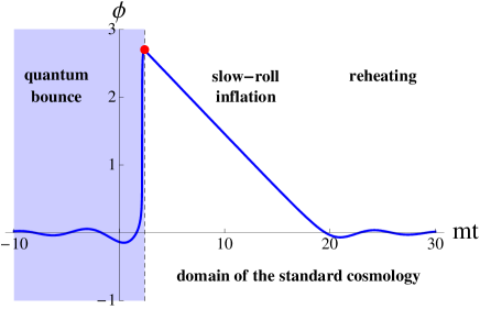
Figure 1: Shark fin-type evolution of a scalar field for $m=10^{-3}m_{\text{Pl}}$. The (red) dot represents the point where the initial conditions in classical cosmology are usually set.

To some extent, it is therefore reasonable to say that the LQC framework solves both the two main ”problems” of the big bang theory: the singularity (which is regularized and replaced by a bounce) and the initial conditions for inflation (which are naturally set by the antifriction term).

However, this shark fin evolution (see caption of Fig. 1) is not the only possible one. In particular, a nearly symmetric evolution can also take place, as studied in Ref. Chiou:2010nd . Those different scenarios can be distinguished by the fraction of kinetic energy at the bounce. When the energy density at the bounce is purely kinetic, the evolution of the field is symmetric. When a small fraction of potential energy is introduced, which is the general case, the symmetry is broken and the field behaves as in the shark fin case. It is however important to underline that we consider only scenarios where the contribution from the potential is subdominant at the bounce, as it would otherwise be necessary to include quantum backreaction effects bojo:back . The effective dynamics would then be more complicated and could not be anymore described by Eq. (1).

In order to perform qualitative studies of the dynamics of the model, it is useful to introduce the variables

$$x:=\frac{m\phi}{\sqrt{2\rho_{\text{c}}}}\ \text{and}\ y:=\frac{\dot{\phi}}{\sqrt{2\rho_{\text{c}}}}.$$ (4)

Since the energy density of the field is constrained ($\rho\leq\rho_{\text{c}}$), the inequality

$$x^{2}+y^{2}\leq 1$$ (5)

has to be fulfilled. The $x^{2}$ term corresponds to the potential part while the $y^{2}$ corresponds to the kinetic term. The case $x^{2}+y^{2}=1$ corresponds to the bounce, when the energy density reaches its maximum.

In Fig. 2, exemplary evolutionary paths in the $x-y$ phase plane are shown.

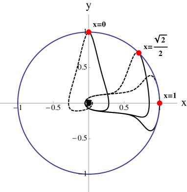
Figure 2: Exemplary phase trajectories of the scalar field with $m=m_{\text{Pl}}$.

For all the presented cases, the evolution begins at the origin (in the limit $t\rightarrow-\infty$), and then evolves (dashed line) to the point on the circle $x^{2}+y^{2}=1$. Finally, the field moves back to the origin for $t\rightarrow+\infty$ (solid line). However, the shapes of the intermediate paths are different. The $x=0$ case corresponds to the symmetric evolution which was studied in Ref. Chiou:2010nd (if the bounce is set at $t=0$, the scale factor is an even function of time and the scalar field is an odd function). In this case, the field is at the bottom of the potential well exactly at the bounce ($H=0$). This is however a very special choice of initial conditions. In the case $x=\sqrt{2}/2$, the potential term and kinetic term contribute equally at the bounce. In this case, both deflation and inflation occur. However one observes differences in their duration. The third case, $x=1$, corresponds to the domination of the potential part at the bounce. In this case, symmetric phases of deflation and inflation also occur (both the scale factor and the field being this time even functions). However in this situation, as well as in $x=\sqrt{2}/2$ case, the effect of quantum backreaction should be taken into account. The dynamics can therefore significantly differ from the one computed with Eq. (1).

In Fig. 3 we show some exemplary evolutions of the scalar field for different contributions from the potential part at the bounce.

Figure 3: Time evolution of the scalar field. Different evolutionary scenarios leading to a slow-roll inflation phase are displayed. The bottom (solid) line represents the symmetric case. The middle (dotted) line represents the shark fin-type evolution mostly investigated in this paper. The top (dashed) line corresponds to a larger fraction of potential energy. For all curves $m=0.01m_{\text{Pl}}$.

In Fig. 4, the corresponding evolutions of the scale factor are displayed.

Figure 4: Time evolution of the scale factor. Different evolutionary scenarios leading to a slow-roll inflation phase are displayed. The bottom (solid) line represents the symmetric case. The middle (dotted) line represents the shark fin type evolution. The top (dashed) line corresponds to a larger fraction of potential energy. For all curves $m=0.01m_{\text{Pl}}$.

It can easily be seen that the value of $\phi_{\text{max}}$ increases with the fraction of potential energy at the bounce. Since the total energy density is constrained, $\phi_{\text{max}}$ must satisfy

$$|\phi_{\text{max}}|\leq\frac{\sqrt{2\rho_{\text{c}}}}{m}.$$ (6)

The values of $\phi_{\text{max}}$ associated with different evolutionary scenarios were computed in Ashtekar:2009mm ; Mielczarek:2009zw ; Chiou:2010nd . The conclusion of those studies is that the necessary conditions for inflation are generically met. Only in the case of a symmetric evolution does the value of $\phi_{\text{max}}$ become too small in some cases. In particular, for $m=10^{-6}m_{\text{Pl}}$ one obtains $\phi_{\text{max}}=2.1m_{\text{Pl}}$ for a symmetric evolution. The corresponding number of e-folds can be computed with $N\simeq 2\pi\frac{\phi^{2}}{m^{2}_{\text{Pl}}}$, which gives $N\simeq 28$. By introducing a small fraction of potential energy (as in the shark fin case), the number of e-folds can be appropriately increased. In addition to the usual arguments, this requirement is also set by the recent WMAP 7-Years results wmap . Based on those observations, the value of the scalar spectral index was indeed measured to be $n_{\text{S}}=0.963\pm 0.012$. As, for a massive slow-roll inflation the relation

$$n_{\text{S}}=1-\frac{1}{\pi}\frac{m^{2}_{\text{Pl}}}{\phi^{2}}$$ (7)

holds, one obtains $\phi_{\text{obs}}=2.9\pm 0.5m_{\text{Pl}}$. Since the consistency relation $\phi_{\text{max}}>\phi_{\text{obs}}$ must be fulfilled, the symmetric evolution with $m=10^{-6}m_{\text{Pl}}$ (for which $\phi_{\text{max}}=2.1m_{\text{Pl}}<\phi_{\text{obs}}$) is not favored by the WMAP 7-Years observations. As already mentioned, higher values of $\phi$ can be easily reached if some contribution from the potential term is introduced (this supports the shark fin scenario). The number of e-folds will therefore be naturally increased in this way. However it remains bounded by above: since $N\simeq 2\pi\frac{\phi^{2}}{m^{2}_{\text{Pl}}}$, Eq. (6) leads to the constrain:

$$N\leq\frac{4\pi\rho_{\text{c}}}{m^{2}m^{2}_{\text{Pl}}}.$$ (8)

The value of the parameter $\rho_{\text{c}}$ can be fixed by Eq. (2). However, this expression is based on the computation of the area gap as performed in LQG. This, in general, can be questioned Dzierzak:2008dy . In particular, in the framework of reduced phase space quantization of LQC, the value of $\rho_{\text{c}}$ remains a free parameter Malkiewicz:2009zd . Moreover, a particular value of the Barbero-Immirzi parameter (imposed by black hole entropy considerations) has been used. Therefore, the value of $\rho_{\text{c}}$ can, in general, differ and it is worth investigating how the variation of $\rho_{\text{c}}$ can alter the dynamics of the model. In particular, we have studied how the shark fin scenario can be modified by different choices of $\rho_{\text{c}}$. In Fig. 5, the evolution of the field is displayed as a function of the value of the critical energy density. As expected, the larger $\rho_{\text{c}}$, the higher the maximum value reached by the field. It can be seen that $\phi_{\text{max}}$ approaches the usually required value $\sim 3m_{\text{Pl}}$ for $\rho_{\text{c}}\sim m^{4}_{\text{Pl}}$, making the whole scenario quite natural.

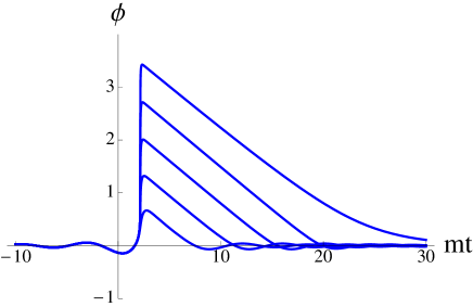
Figure 5: The shark fin-type evolution of the scalar field for $m=10^{-3}m_{\text{Pl}}$. Curves from bottom to top were computed for $\rho_{\text{c}}=10^{-6},10^{-4},10^{-2},1,$ and $100\ [m^{4}_{\text{Pl}}],$ respectively.

III Gravitational waves in LQC

Although quite a lot of work has already been devoted to gravitational waves in LQC lqcgen , this study aims at treating, for the first time, the problem in a fully self-consistent way with an explicit emphasis on the investigation of the spectrum that can be used as an input to study possible experimental signatures.

The equation for tensor modes in LQC is given (see, e.g., Bojowald:2007cd ) by

$$\frac{d^{2}}{d\eta^{2}}h^{i}_{a}+2aH\frac{d}{d\eta}h^{i}_{a}-\nabla^{2}h^{i}_{a}+m^{2}_{Q}h^{i}_{a}=0,$$ (9)

where $h^{i}_{a}$ are gravitational perturbations, $\eta$ is the conformal time and the factor due to the holonomy corrections is given by

$$m^{2}_{Q}:=16\pi Ga^{2}\frac{\rho}{\rho_{c}}\left(\frac{2}{3}\rho-V\right).$$ (10)

This factor acts as an effective mass term. For convenience we introduce the variable

$$u=\frac{ah_{\oplus}}{\sqrt{16\pi G}}=\frac{ah_{\otimes}}{\sqrt{16\pi G}},$$ (11)

where $h^{1}_{1}=-h^{2}_{2}=h_{\oplus}$, $h^{1}_{2}=h^{2}_{1}=h_{\otimes}$. Then, performing the Fourier transform

$$u({\bf x},\eta)=\int\frac{d^{3}{\bf k}}{(2\pi)^{3}}u_{\bf k}(\eta)e^{i{\bf k}\cdot{\bf x}},$$ (12)

one can rewrite the equation as

$$\frac{d^{2}}{d\eta^{2}}u_{\bf k}(\eta)+\left[k^{2}+m^{2}_{\text{eff}}\right]u_{\bf k}(\eta)=0,$$ (13)

where $k^{2}={\bf k}\cdot{\bf k}$ and

$$m^{2}_{\text{eff}}:=m^{2}_{Q}-\frac{a^{{}^{\prime\prime}}}{a}=a^{2}\frac{\kappa}{2}\left[p-\frac{1}{3}\rho\right].$$ (14)

It is worth underlining that the final expression of $m_{\text{eff}}$ has no explicit dependence upon the critical energy density $\rho_{\text{c}}$. In Eq. (14), both $m^{2}_{Q}$ and $a^{{}^{\prime\prime}}/a$ depend on $\rho_{\text{c}}$. However since

$$\frac{a^{{}^{\prime\prime}}}{a}=a^{2}\left[\frac{2\kappa}{3}\rho\left(1-\frac{\rho}{\rho_{\text{c}}}\right)-\frac{\kappa}{2}(\rho+p)\left(1-\frac{2\rho}{\rho_{\text{c}}}\right)\right],$$ (15)

the factors depending on $\rho_{\text{c}}$ cancel out precisely. This is perhaps not a coincidence and this could exhibit the conservation of classical symmetries while introducing the quantum corrections.

The next step consists in quantizing the Fourier modes $u_{\bf k}(\eta)$. This follows the standard canonical procedure. Promoting this quantity to be an operator, one performs the decomposition

$$\hat{u}_{\bf k}(\eta)=f_{k}(\eta)\hat{b}_{\bf k}+f_{k}^{*}(\eta)\hat{b}^{\dagger}_{\bf-k},$$ (16)

where $f_{k}(\eta)$ is the so-called mode function which satisfies the same equation as $u_{\bf k}(\eta)$, namely Eq. (13). The creation ($\hat{b}^{\dagger}_{\bf k}$) and annihilation ($\hat{b}_{\bf k}$) operators fulfill the commutation relation $[\hat{b}_{\bf k},\hat{b}^{\dagger}_{\bf q}]=\delta^{(3)}({\bf k-q})$.

The problem is now shifted to the resolution of a Schrödinger-like Eq. (13) which can be used to compute the observationally relevant quantities. In particular, the correlation function for tensor modes is given by

$$\langle 0|\hat{h}^{a}_{b}({\mathbb{x}},\eta)\hat{h}^{b}_{a}({\mathbb{y}},\eta)|0\rangle=\int_{0}^{\infty}\frac{dk}{k}\mathcal{P}_{\text{T}}(k,\eta)\frac{\sin kr}{kr},$$ (17)

where $\mathcal{P}_{\text{T}}$ is the tensor power spectrum and $|0\rangle$ is the vacuum state. In our case, $\mathcal{P}_{\text{T}}$ can be written as

$$\mathcal{P}_{\text{T}}(k,\eta)=\frac{64\pi G}{a^{2}(\eta)}\frac{k^{3}}{2\pi^{2}}|f_{k}(\eta)|^{2}.$$ (18)

This spectrum is the fundamental observable associated with gravitational wave production. As will be shown in the next sections, very substantial deviations from the usual shape are to be expected within the LQC framework.

IV Analytical investigation of the power spectrum

In this section we perform analytical studies of gravitational wave creation in the scenario previously described. In particular, we derive approximate formulas for the tensor power spectrum at the end of inflation. In the next section we will compare this result with numerical computations.

In the considered model, the evolution is split into three parts: contraction, bounce and slow-roll inflation. For this model, the effective mass square is defined as follows

$$m^{2}_{\text{eff}}(\eta)=\left\{\begin{array}[]{ccc}0&\text{for}&\eta<\eta_{i}-\Delta\eta.\\ k_{0}^{2}&\text{for}&\eta_{i}-\Delta\eta<\eta<\eta_{i}.\\ -\left(\nu^{2}-\frac{1}{4}\right)\frac{1}{\eta^{2}}&\text{for}&\eta>\eta_{i}.\end{array}\right.$$ (19)

Basically, the phenomenological parameters entering the model are therefore:

• $\eta_{i}$ — the beginning of the inflation.

• $\Delta\eta$ — the width of the bounce.

• $k_{0}$ — which is approximately equal to the value of $m_{\text{eff}}$ at the bounce (when $H=0$). It can therefore be related with the energy scale of the bounce.

• $\nu$ — which is related to slow-roll parameter $\epsilon$ by $\nu=\sqrt{\frac{9}{4}+3\epsilon}=\frac{3}{2}+\epsilon+\mathcal{O}(\epsilon^{2})$, where $\epsilon\ll 1$.

For the considered model, we have $k^{2}_{0}\geq 0$. This comes from the fact that we consider the particular shark fin-type of evolution where the bounce is dominated by the kinetic energy term. Therefore when $y\gg x$ [see Eq. (4)], Eq. (14) simplifies to $m^{2}_{\text{eff}}=a^{2}\kappa\dot{\phi}^{2}/6\geq 0$, leading to $k^{2}_{0}\approx m^{2}_{\text{eff}}(t=t_{\text{bounce}})\geq 0$.

A matching should be performed between the three considered phases. It can be done, as displayed in Fig. 6, with transition matrices defined as follows:

$${\bf M}:=\left[\begin{array}[]{cc}f_{k}(\eta)&f^{*}_{k}(\eta)\\ \partial_{\eta}f_{k}(\eta)&\partial_{\eta}f^{*}_{k}(\eta)\end{array}\right],$$ (20)

where the Wronskian condition implies

$$W(f_{k}(\eta),f^{*}_{k}(\eta)):=\det{\bf M}=i.$$ (21)

The inverse of the transition matrix is then given by:

$${\bf M}^{-1}:=-i\left[\begin{array}[]{cc}\partial_{\eta}f^{*}_{k}(\eta)&-f^{*}_{k}(\eta)\\ -\partial_{\eta}f_{k}(\eta)&f_{k}(\eta)\end{array}\right].$$ (22)

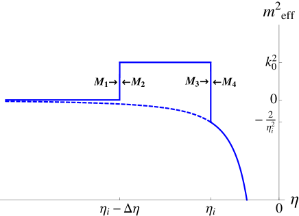
Figure 6: Evolution of the effective mass used in the analytical approximation [Eq. (19)]. On this plot, $\epsilon$ is set to zero as an example. The dashed line represents the case without a bounce. The points where the transfer matrices are computed in our model are also indicated.

The three first transition matrices are:

$${\bf M_{1}} = \left[\begin{array}[]{cc}\frac{e^{-ik(\eta_{i}-\Delta\eta)}}{\sqrt{2k}}&\frac{e^{ik(\eta_{i}-\Delta\eta)}}{\sqrt{2k}}\\ -i\sqrt{\frac{k}{2}}e^{-ik(\eta_{i}-\Delta\eta)}&i\sqrt{\frac{k}{2}}e^{ik(\eta_{i}-\Delta\eta)}\end{array}\right],$$ (25)

$${\bf M_{2}} = \left[\begin{array}[]{cc}\frac{e^{-i\Omega(\eta_{i}-\Delta\eta)}}{\sqrt{2\Omega}}&\frac{e^{i\Omega(\eta_{i}-\Delta\eta)}}{\sqrt{2\Omega}}\\ -i\sqrt{\frac{\Omega}{2}}e^{-i\Omega(\eta_{i}-\Delta\eta)}&i\sqrt{\frac{\Omega}{2}}e^{i\Omega(\eta_{i}-\Delta\eta)}\end{array}\right],$$ (28)

$${\bf M_{3}} = \left[\begin{array}[]{cc}\frac{e^{-i\Omega\eta_{i}}}{\sqrt{2\Omega}}&\frac{e^{i\Omega\eta_{i}}}{\sqrt{2\Omega}}\\ -i\sqrt{\frac{\Omega}{2}}e^{-i\Omega\eta_{i}}&i\sqrt{\frac{\Omega}{2}}e^{i\Omega\eta_{i}}\end{array}\right],$$ (31)

where

$$\Omega=\sqrt{k^{2}+k^{2}_{0}}.$$ (32)

In the last region, mode functions can be written as

$$f_{k}(\eta)=\alpha_{k}g_{k}(\eta)+\beta_{k}g^{*}_{k}(\eta),$$ (33)

where

$$g_{k}(\eta)=\sqrt{-\eta}\sqrt{\frac{\pi}{4}}e^{i\pi(2\nu+1)/4}H^{(1)}_{\nu}(-k\eta),$$ (34)

$H_{\nu}(x)$ being a Hankel function of the first kind. The mode functions $g_{k}(\eta)$ correspond to another decomposition of the field $\hat{u}_{\bf k}(\eta)$ in the form:

$$\hat{u}_{\bf k}(\eta)=g_{k}(\eta)\hat{a}_{\bf k}+g_{k}^{*}(\eta)\hat{a}^{\dagger}_{\bf-k}.$$ (35)

The creation ($\hat{a}^{\dagger}_{\bf k}$) and annihilation ($\hat{a}_{\bf k}$) operators fulfill the commutation relation $[\hat{a}_{\bf k},\hat{a}^{\dagger}_{\bf q}]=\delta^{(3)}({\bf k-q})$. Because decompositions (16) and (35) are equivalent, based on Eq. (33) and on the Wronskian conditions for the mode functions $f_{k}$ and $g_{k}$, one obtains:

$$\left[\begin{array}[]{c}\hat{b}_{\bf k}\\ \hat{b}^{\dagger}_{\bf-k}\end{array}\right]=\left[\begin{array}[]{cc}\alpha_{k}&\beta_{k}^{*}\\ \beta_{k}&\alpha^{*}_{k}\end{array}\right]\left[\begin{array}[]{c}\hat{a}_{\bf k}\\ \hat{a}^{\dagger}_{\bf-k}\end{array}\right],$$ (36)

which corresponds to a Bogoliubov transformation with coefficients $\alpha_{k}$ and $\beta_{k}$. Because of the commutation relation of the creation and annihilation operators we have $|\alpha_{k}|^{2}-|\beta_{k}|^{2}=1$. It is clear from Eq. (36) that if $\beta_{k}\neq 0$ particles are created from the vacuum, just because $\hat{b}_{\bf k}|0\rangle=\beta_{k}^{*}\hat{a}^{\dagger}_{\bf-k}|0\rangle$. By matching the three regions, the unknown coefficients $\alpha_{k}$ and $\beta_{k}$ can be determined:

$$\left[\begin{array}[]{c}\alpha_{k}\\ \beta_{k}\end{array}\right] = {\bf M_{4}}^{-1}{\bf M_{3}}{\bf M_{2}}^{-1}{\bf M_{1}}\left[\begin{array}[]{c}1\\ 0\end{array}\right]$$ (41)

$$= {\bf M_{4}}^{-1}\left[\begin{array}[]{c}\frac{e^{ik(\Delta\eta-\eta_{i})}(\Omega\cos[\Delta\eta\Omega]-ik\sin[\Delta\eta\Omega])}{\sqrt{2k}\Omega}\\ \frac{e^{ik(\Delta\eta-\eta_{i})}(-ik\cos[\Delta\eta\Omega]-\Omega\sin[\Delta\eta\Omega])}{\sqrt{2k}}\end{array}\right],$$ (44)

where ${\bf M_{4}}$ is given by

$${\bf M_{4}}=\left[\begin{array}[]{cc}g_{k}(\eta)&g^{*}_{k}(\eta)\\ \partial_{\eta}g_{k}(\eta)&\partial_{\eta}g^{*}_{k}(\eta)\end{array}\right]_{\eta=\eta_{i}},$$ (45)

the mode function $g_{k}$ being given by Eq. (34). In the special case corresponding to a de Sitter inflation ($\epsilon=0$ and $\nu=\frac{3}{2}$), the mode functions given by Eq. (34) simplify to the Bunch-Davies vacuum

$$\left.g_{k}(\eta)\right|_{\nu=\frac{3}{2}}=g^{\text{B-D}}_{k}(\eta)=\frac{e^{-ik\eta}}{\sqrt{2k}}\left(1-\frac{i}{k\eta}\right).$$ (46)

In general, the amplitude of the mode function during inflation can be written as

$$|f_{k}|^{2}=|g_{k}|^{2}|\alpha_{k}-\beta_{k}|^{2}+4\Re(\alpha_{k}^{*}\beta_{k}g_{k}^{*})\Re{g_{k}}.$$ (47)

As we are interested in the spectrum at the end of inflation ($\eta\rightarrow 0^{-}$), the approximation

$$H^{(1)}_{\nu}(x)\simeq-\frac{i}{\pi}\Gamma(\nu)\left(\frac{x}{2}\right)^{-\nu}$$ (48)

holds and, based on this, one can easily see that for a slow-roll inflation ($\epsilon\ll 1$):

$$\lim_{\eta\rightarrow 0^{-}}\frac{\Re{g_{k}(\eta)}}{\Im{g_{k}(\eta)}}=\mathcal{O}(\epsilon).$$ (49)

Therefore, the leading order contribution from Eq. (47) becomes

$$\lim_{\eta\rightarrow 0^{-}}|f_{k}|^{2}=|g_{k}|^{2}|\alpha_{k}-\beta_{k}|^{2}.$$ (50)

With this approximation, the tensor power spectrum at the end of inflation takes the form

$$\mathcal{P}_{\text{T}}(k)=\frac{16}{\pi}\left(\frac{H}{m_{\text{Pl}}}\right)^{2}\left(\frac{k}{aH}\right)^{-2\epsilon}|\alpha_{k}-\beta_{k}|^{2}.$$ (51)

The coefficients $\alpha_{k}$ and $\beta_{k}$ are computed from Eq. (41). Since the resulting expression for $|\alpha_{k}-\beta_{k}|^{2}$ is very long, it is not explicitly given here. It exhibits the correct ultra-violet (UV) behavior, namely $\lim_{k\rightarrow\infty}|\alpha_{k}-\beta_{k}|^{2}=1$. Therefore, the UV spectrum simplifies to

$$\mathcal{P}_{\text{T}}(k\to\infty)=\frac{16}{\pi}\left(\frac{H}{m_{\text{Pl}}}\right)^{2}\left(\frac{k}{aH}\right)^{-2\epsilon}.$$ (52)

In Fig. 7, spectra, as obtained from Eq. (51), are displayed for different values of $k_{0}$ and normalized to the usual non-LQC corrected spectrum. In Fig. 8, the width of the bounce $\Delta\eta$ is varied. In both cases, $\epsilon$ is vanishing.

Figure 7: Analytical tensor power spectra, normalized to the non-LQC-corrected spectrum, for three different values of $k_{0}$ in the $\epsilon=0$ case. The parameters are: $k_{0}=0$ (solid line), $k_{0}=1.5$ (dashed line), $k_{0}=3$ (dotted line), $\eta_{i}=-1$, and $\Delta\eta=1$.

Figure 8: Analytical tensor power spectra, normalized to the non-LQC-corrected spectrum, for two different values of $\Delta\eta$ in the $\epsilon=0$ case. The parameters are: $\Delta\eta=0$ (solid line), $\Delta\eta=10$ (dashed line), $k_{0}=1$, and $\eta_{i}=-1$.

The main features that can be drawn from those plots are the following:

• The power is suppressed in the infra-red (IR) regime. This is a characteristic feature associated with the bounce.

• The UV behavior agrees with the standard general relativistic picture.

• Damped oscillations are superimposed with the spectrum around the ”transition” momentum $k_{*}$ between the suppressed regime and the standard regime.

• The first oscillation behaves like a ”bump” that can substantially exceed the UV asymptotic value.

• The parameter $k_{0}$ basically controls the amplitude of the oscillations whereas $\Delta\eta$ controls their frequency.

V Numerical investigation of the power spectrum

To perform a more detailed analysis, we have also fully numerically solved the system of coupled differential equations which leads to both the evolution of the modes and of the background:

$$\frac{d^{2}f_{k}}{dt^{2}} = -H\frac{df_{k}}{dt}-\left[\frac{k^{2}}{a^{2}}+\frac{\kappa}{6}\left(3p-\rho\right)\right]f_{k},$$ (53)

$$\frac{dH}{dt} = \frac{1}{2}\kappa(\rho+p)\left(2\frac{\rho}{\rho_{c}}-1\right),$$ (54)

$$\frac{da}{dt} = Ha,$$ (55)

$$\frac{d\phi}{dt} = \frac{\pi_{\phi}}{a^{3}},$$ (56)

$$\frac{d\pi_{\phi}}{dt} = -a^{3}\phi,$$ (57)

where

$$\rho=\frac{\pi^{2}_{\phi}}{2a^{6}}+\frac{m^{2}}{2}\phi^{2}\ \text{and}\ p=\frac{\pi^{2}_{\phi}}{2a^{6}}-\frac{m^{2}}{2}\phi^{2}$$ (58)

are respectively the energy density and pressure of the scalar field whereas $\pi_{\phi}$ is the momentum.

To compute the evolution of the modes, the initial condition was assumed to be the Minkowski vacuum

$$f_{k}=\frac{e^{-ik\eta}}{\sqrt{2k}}.$$ (59)

This approximation is valid for the subhorizontal modes. Therefore, in the numerical computations we have evolved only modes that were subhorizontal at the initial time.

In Fig. 9, the analytical spectrum Eq. (51) evaluated as explained in the previous section is compared with the full numerical computation. The overall agreement is very good with slight deviations due to subtle dynamical effects. The UV tilt associated with the slow-roll parameter is perfectly recovered. The values of parameters $H$, $k_{0}$ and $\epsilon$ were determined from the evolution of the background. In turn, the parameters $\eta_{i}$ and $\Delta\eta$ were fixed to fit the numerical data.

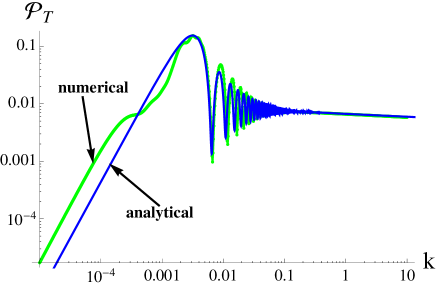
Figure 9: Comparison of numerical and analytical spectra Eq. (51) for $m=10^{-2}m_{\text{Pl}}$. In the IR region the spectra behave as $\mathcal{P}_{\text{T}}\propto k^{2}$ while in the UV region they behave as $\mathcal{P}_{\text{T}}\propto k^{-2\epsilon}$, where $\epsilon\ll 1$ is the slow-roll parameter. Here: $H=0.037m_{\text{Pl}},\epsilon=0.0246,k_{0}=0.037m_{\text{Pl}},\eta_{i}=-750,$ and $\Delta\eta=10$.

The mass of the scalar field is, of course, the key physical parameter of this model. The canonically chosen value (around $10^{-6}m_{\text{Pl}}$) may not be especially meaningful in this approach as the standard requirements of inflation are substantially modified by the specific history of the Hubble radius. This value is nonetheless still the mostly preferred one.

In Fig. 10, the spectra computed for three different mass values are displayed. As expected, the UV value of the spectrum scales as $m^{2}$, since during inflation $\mathcal{P}_{\text{T}}\sim H^{2}\sim m^{2}$.

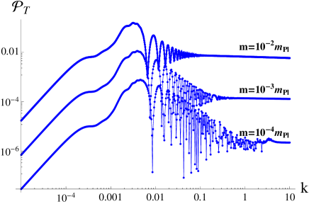
Figure 10: Numerically computed power spectra for $m=10^{-4},10^{-3},10^{-2}$ $m_{\text{Pl}}$ (from bottom to top in the UV range).

It is also clear that the region of oscillations becomes broader while lowering the value of $m$.

In Fig. 11, we show how the spectrum is modified by different choices of $\rho_{\text{c}}$.

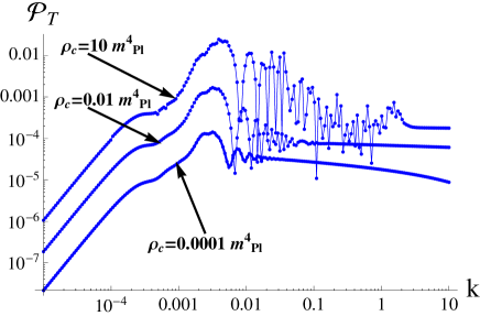
Figure 11: Numerically computed power spectra for $\rho_{\text{c}}=10^{-4},10^{-2},10$ $m^{4}_{\text{Pl}}$ (from bottom to top in the UV range) with $m=10^{-3}m_{\text{Pl}}$.

It is clear that increasing $\rho_{\text{c}}$ leads to an amplification of the spectrum. The dependence is however not very strong. As it was shown in Section II, the increase of $\rho_{\text{c}}$ leads to an increase of the field displacement $\phi_{\text{max}}$. This dependence was shown to be rather weak. Since $\mathcal{P}_{\text{T}}\sim H^{2}\sim m^{2}\phi^{2}$, the increase of $\phi$ due to the dependence upon $\rho_{\text{c}}$ will result in an amplification of the power spectrum. This is in agreement with the numerical results. From Fig. 11, it can also be noticed that increasing $\rho_{\text{c}}$ amplifies the oscillatory structure.

The numerical investigations performed for this work have shown that the quantity $R$ defined as

$$R:=\frac{\mathcal{P}_{\text{T}}(k=k_{*})}{\mathcal{P}^{\text{standard}}_{\text{T}}(k=k_{*})},$$ (60)

basically evolves as

$$R\simeq\left(\frac{m_{\text{Pl}}}{m}\right)^{0.64},$$ (61)

where $k_{*}$ is the position of the highest peak in the power spectrum and $\mathcal{P}^{\text{standard}}_{\text{T}}(k)$ is a standard inflationary power spectrum [see e.g. Eq. (52)] which overlaps with $\mathcal{P}_{\text{T}}(k)$ for $k\rightarrow\infty$. The function (61) was obtained by fitting the numerical data in the mass range $m=5\cdot 10^{-5}m_{\text{Pl}}\ ...\ 10^{-1}m_{\text{Pl}}$. Because of numerical instabilities, it was not possible to perform computations for lower values of the inflaton mass. The numerically obtained values of $R$ together with the approximation given by Eq. (61) are given in Fig. 12.

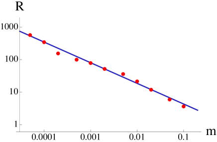
Figure 12: Ratio defined by Eq. (60) as a function of inflaton mass in Planck units. Dots are values obtained from the numerical computations. The straight line is the fit given by Eq. (61).

This parametrization is useful for phenomenological purposes. Interestingly, $R$ can become very high for low values of the mass of the field. This partially compensates for the lower overall normalization of the spectrum and can become a very specific feature of the model. In particular, for the mass $m\approx 10^{-6}m_{\text{Pl}}$ (which is the value preferred by some estimations), extrapolating the relation (61) leads to $R\approx 8000$. If the relation still holds in this range, the effect is very significant, and could have important observational consequences.

Finally, to make basic studies easier, we performed a rough parametrization of the full spectrum:

$$\mathcal{P}_{\text{T}}=\frac{16}{\pi}\left(\frac{H}{m_{\text{Pl}}}\right)^{2}\frac{\left(\frac{k}{aH}\right)^{-2\epsilon}}{1+(k_{*}/k)^{2}}\left[1+\frac{4R-2}{1+(k/k_{*})^{2}}\right],$$ (62)

leading to

$$\mathcal{P}^{\text{dS}}_{\text{T}}=\frac{16}{\pi}\left(\frac{H}{m_{\text{Pl}}}\right)^{2}\frac{1}{1+(k_{*}/k)^{2}}\left[1+\frac{4R-2}{1+(k/k_{*})^{2}}\right],$$ (63)

in the specific case of de Sitter inflation. In both cases, the classical behavior is recovered in the limit $k\rightarrow\infty$. The point for introducing the $R$ factor the way it was done becomes clear when calculating the value of the spectra at $k=k_{*}$. For a modified de Sitter spectrum [Eq. (63)], we get

$$\mathcal{P}^{\text{dS}}_{\text{T}}(k=k_{*})=R\frac{16}{\pi}\left(\frac{H}{m_{\text{Pl}}}\right)^{2}.$$ (64)

Thanks to the relation (61), the number of the free parameters can be decreased in a phenomenological analysis.

As shown on Fig. 13, this formula correctly reproduces the main features, namely the IR power suppression, the bump and the UV limit. Oscillations are missed but due to momentum integration there is little hope that they can observationally be seen on a cosmological microwave background (CMB) spectrum.

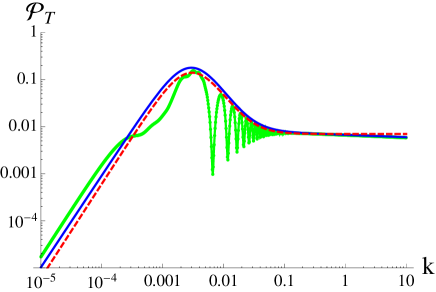
Figure 13: Comparison of the numerical spectrum for $m=10^{-2}m_{\text{Pl}}$ with formulas (62) and (63). The solid (blue) line corresponds to (62) while the dashed (red) line corresponds to (63).

To conclude this section, we have schematically represented the evolution of the Hubble radius ($R_{\text{H}}:=1/|H|$), together with the physical modes, in Fig. 14. This helps to understand the shape of the obtained spectra.

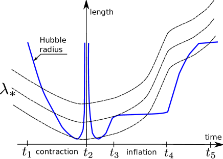
Figure 14: Schematic picture of evolution of the Hubble radius (solid line) and of the different length scales (dashed lines) for the considered model of the universe. Different times are distinguished: $t_{1}-$time when the initial conditions are set; $t_{2}-$bounce ($H=0$); $t_{3}-$beginning of inflation; $t_{4}-$end of inflation; $t_{5}-$present epoch of dark energy domination.

We consider the modes that are initially (at time $t_{1}$) shorter than the Hubble radius. For those modes, the normalized solution is given by the Minkowski vacuum $f_{k}=e^{-ik\eta}/\sqrt{2k}$. Therefore, the initial power spectrum takes the form $\mathcal{P}_{\text{T}}\sim k^{3}|f_{k}|^{2}\sim k^{2}$. Starting from the largest scales, the modes cross the Hubble radius. This is possible since the Hubble radius undergoes contraction faster than any particular length scale. While crossing the horizon, the shape of the spectrum becomes frozen in the initial $\mathcal{P}_{\text{T}}\sim k^{2}$ form. Then, the modes evolve through the bounce (at time $t_{2}$) until the beginning of inflation (at time $t_{3}$). The main consequence of the transition of modes through the bounce is the appearance of additional oscillations in the spectrum. This issue was studied in detail in Ref. Mielczarek:2009vi , where the spectrum at time $t_{3}$ was calculated for the symmetric bounce model. After the bounce, modes with wavelengths shorter than $\lambda_{*}$ start to reenter the Hubble radius. The superhorizon modes $\lambda>\lambda_{*}$ ($k<k_{*}$) hold the $k^{2}$ spectrum, with however some oscillatory features due to the bounce. Modes with $\lambda<\lambda_{*}$ ($k>k_{*}$) cross the horizon again during the phase of inflation. For them, the spectrum agrees with the standard slow-roll inflation spectrum $\mathcal{P}_{\text{T}}\sim k^{-2\epsilon}$ where $\epsilon\ll 1$. The small tilt is due to a slow increase of the Hubble radius. Contributions from different modes are then slightly different. At the end of inflation (at time $t_{4}$) the spectrum is therefore suppressed ($\mathcal{P}_{\text{T}}\sim k^{2}$) for $k<k_{*}$ and exhibits the inflationary shape ($\mathcal{P}_{\text{T}}\sim k^{-2\epsilon}$) for $k>k_{*}$. The spectrum is also modified by the oscillations due to the bounce. This corresponds to the computations of this paper. The particular mode with wavelength $\lambda_{*}$ (wave number $k_{*}$) should be studied in more detail. The size of this mode overlaps with the size of the Hubble radius at the beginning of inflation: $k_{*}\simeq a(t_{3})H(t_{3})$. The physical length $\lambda_{*}$ at the scale factor $a(t)$ is therefore equal to $\lambda_{*}(t)\simeq a(t)/[a(t_{3})H(t_{3})]$. This scale grows with the cosmic expansion and it is crucial, from the observational point of view, to determine its present size (at time $t_{5}$). The case drawn in Fig. 14 corresponds to a present size of $\lambda_{*}$ greater than the size of the horizon. This is indeed rather unlikely that the present value of $\lambda_{*}$ is below the size of horizon just because the spectrum of scalar perturbations should then exhibit deviations from the nearly scale invariant inflationary prediction. Up to now, there is no observational evidence for such deviations. A remaining possibility would however be that the (slight) observed lack of power in the CMB spectrum of anisotropies could be due to the effects of the bounce. However, the present size of $\lambda_{*}$ would then be comparable with the size of horizon. This leads to the question: why should those two scales overlap right now? This is rather unnatural, and would lead to a new coincidence problem. However, as it was estimated in Ref. Mielczarek:2009zw , these two scales can indeed overlap in the standard inflationary scenario for quite natural values of the parameters. There is therefore a glimpse of hope that the scale $\lambda_{*}$ is at least not to much bigger than the size of horizon. This could allow us to see some UV features due to the bounce as the oscillations also affect sightly the inflationary part of the spectrum. These are however secondary effects and it is not clear whether they were not smoothed away during the radiation domination era. Moreover, in the region where those effects could be expected, errors due to the cosmic variance become significant. This is an unavoidable observational limitation which cannot be bettered, even by the improvement of resolution of the future CMB experiments.

Another limitation in studying the effects of LQC comes from the fact that the derived modifications can also appear in other bouncing cosmologies. In particular, within the model of quintom bounce, the discussed effects of suppression and oscillations were also pointed out Cai:2008ed ; Cai:2008qb . The amplitude of tensor perturbations at the peak was however not predicted to be as high as in LQC. An additional amplification on the very large scales was also predicted in the quintom model. Despite these differences, at the observationally accessible low scales, the effects due to the LQC bounce and the quintom bounce are mostly indistinguishable. Therefore, complementary observational methods have to be proposed to distinguish between such models. A possible distinction could be given e.g. from the analysis of non-Gaussianity production within LQC.

VI Conclusions

This study establishes the full background dynamics in bouncing models with holonomy corrections. Although this has already been claimed before, we confirm that due to the sudden change of sign of the Hubble parameter, inflation is nearly unavoidable. In this paper, we have considered a particular model of inflation where the content of the universe is dominated by a massive scalar field. We have investigated the details by both analytical and numerical studies the primordial power spectrum of gravitational waves. It exhibits several characteristic features, namely a $\mathcal{P}_{\text{T}}\propto k^{2}$ IR power suppression, oscillations, and a bump at $k_{*}$. In the UV regime, the standard inflationary spectrum $\mathcal{P}_{\text{T}}\propto k^{-2\epsilon}$ is recovered. The primordial tensor power spectrum transforms into $B$-type CMB polarization. The performed investigations therefore open the window for observational tests of the model, in particular through the amplification which occurs while approaching $k\rightarrow k_{*}$. The observed structures correspond to the UV region in the spectrum. If the present scale $\lambda_{*}\sim 1/k_{*}$ is not much larger than the size of horizon, then the effects of the bounce should be, in principle, observable. In particular, one should expect amplification, rather than suppression of the $B$-type polarization spectrum at the low multipoles. The suppression for $k<k_{*}$ becomes dominant at the much larger scale, probably far above the horizon. While the $B$-type polarization has not been detected yet, there are huge efforts in this direction. Experiments such as PLANCK :2006uk , BICEP Chiang:2009xsa or QUIET Samtleben:2008rb are (partly) devoted to the search of the $B$ mode. Even with present observational constraints, one can already exclude some evolutionary scenarios and possible values of the parameters, in particular the inflaton mass $m$ and position of the bump $k_{*}$ in the spectrum. We address this interesting issue elsewhere dream_team . There are also still several points to study around this model:

• How is the scenario modified when quantum backreaction is taken into account (in particular when the potential energy of the field in not negligible at the bounce)?

• How is the power spectrum modified by inverse-volume terms in this framework? Although the background dynamics should not be fundamentally altered, the spectrum could be significantly modified.

• How do those results compare with models dealing with classical bounces (see, e.g., peter )? If the IR power suppression is probably a generic feature of bounces, the detailed features are model-dependent.

Together with the known success of LQC (The singularity resolution, the correct low-energy behavior, etc.), the facts that 1) inflation naturally occurs and 2) observational features can be expected from the model, are strong cases for loop cosmology. Those two points are the main results of this paper.

- (1) C. Rovelli, Quantum Gravity, Cambridge, Cambridge University Press, 2004; C. Rovelli, Living Rev. Relativity, 1, 1 (1998); L. Smolin, arXiv:hep-th/0408048v3; T. Thiemann, Lect. Notes Phys. 631, 41(2003); A. Perez, arXiv:gr-qc/0409061v3.
- (2) M. Bojowald, Living Rev. Rel. 11, 4 (2008); A. Ashtekar, Gen. Rel. Grav. 41, 707 (2009)
- (3) A. Linde, Lect. Notes Phys. 738, 1 (2008).
- (4) E. Komatsu et al., Submitted to Astrophs. J. Suppl. Ser., arXiv:1001.4538v1
- (5) A. Ashtekar and D. Sloan, arXiv:0912.4093 [gr-qc].
- (6) M. Bojowald, Phys. Rev. Lett. 89, 261301 (2002)
- (7) K. A. Meissner, Class. Quant. Grav. 21 (2004) 5245 [arXiv:gr-qc/0407052].
- (8) P. Singh, K. Vandersloot and G. V. Vereshchagin, Phys. Rev. D 74 (2006) 043510 [arXiv:gr-qc/0606032].
- (9) J. Mielczarek, Phys. Rev. D 81 (2010) 063503 [arXiv:0908.4329 [gr-qc]].
- (10) D. W. Chiou and K. Liu, arXiv:1002.2035 [gr-qc].
- (11) M. Bojowald, Phys. Rev. Lett. 100 221301 (2008); M. Bojowald, arXiv:1002.2618 [gr-qc].
- (12) P. Dzierzak, J. Jezierski, P. Malkiewicz and W. Piechocki, Acta Phys. Polon. B 41 (2010) 717 [arXiv:0810.3172 [gr-qc]].
- (13) P. Malkiewicz and W. Piechocki, Phys. Rev. D 80 (2009) 063506 [arXiv:0903.4352 [gr-qc]].
- (14) D. Mulryne and N. Nunes, Phys. Rev. D 74, 083507 (2006); J. Mielczarek and M. Szydlowski, Phys. Lett. B 657, 20 (2007); E. J. Copeland, D. J. Mulryne, N. J. Nunes, and M. Shaeri, Phys. Rev. D 77, 023510 (2008); J. Mielczarek, J. Cosmo. Astropart. Phys. 0811:011 (2008); E. J. Copeland, D. J. Mulryne, N. J. Nunes, and M. Shaeri, Phys. Rev. D 79, 023508 (2009); J. Grain and A. Barrau, Phys. Rev. Lett 102, 081301 (2009); A. Barrau and J. Grain, Proc. of the 43rd Rencontres de Moriond, arXiv:0805.0356v1 [gr-qc]; J. Mielczarek, Phys. Rev .D 79, 123520 (2009); M. Shimano and T. Harada, Phys. Rev. D 80 (2009) 063538; J. Grain, A. Barrau, A. Gorecki, Phys. Rev. D 79, 084015 (2009); J. Grain, arXiv:0911.1625[gr-qc]; A. Barrau, arXiv:0911.3745 [gr-qc]; J. Grain, T. Cailleteau, A. Barrau, A. Gorecki, Phys. Rev. D 81, 024040 (2010).
- (15) M. Bojowald and G. M. Hossain, Phys. Rev. D 77 (2008) 023508 [arXiv:0709.2365 [gr-qc]].
- (16) J. Mielczarek, Phys. Rev. D 79 (2009) 123520 [arXiv:0902.2490 [gr-qc]].
- (17) [Planck Collaboration], arXiv:astro-ph/0604069.
- (18) Y. F. Cai and X. Zhang, JCAP 0906 (2009) 003 [arXiv:0808.2551 [astro-ph]].
- (19) Y. F. Cai, T. t. Qiu, J. Q. Xia and X. Zhang, Phys. Rev. D 79 (2009) 021303 [arXiv:0808.0819 [astro-ph]].
- (20) H. C. Chiang et al., arXiv:0906.1181 [astro-ph.CO].
- (21) D. Samtleben and f. t. Q. Collaboration, Nuovo Cim. 122B (2007) 1353 [arXiv:0802.2657 [astro-ph]].
- (22) J. Grain et al., (unpublished).
- (23) F. T. Falciano, M. Lilley and P. Peter, Phys. Rev. D 77, 083513 (2008).